Global quark polarization in non-central $A+A$ collisions

Abstract

Partons produced in the early stage of non-central heavy-ion collisions can develop a longitudinal fluid shear because of unequal local number densities of participant target and projectile nucleons. Under such fluid shear, local parton pairs with non-vanishing impact parameter have finite local relative orbital angular momentum along the direction opposite to the reaction plane. Such finite relative orbital angular momentum among locally interacting quark pairs can lead to global quark polarization along the same direction due to spin-orbital coupling. Local longitudinal fluid shear is estimated within both Landau fireball and Bjorken scaling model of initial parton production. Quark polarization through quark-quark scatterings with the exchange of a thermal gluon is calculated beyond small-angle scattering approximation in a quark-gluon plasma. The polarization is shown to have a non-monotonic dependence on the local relative orbital angular momentum dictated by the interplay between electric and magnetic interaction. It peaks at a value of relative orbital angular momentum which scales with the magnetic mass of the exchanged gluons. With the estimated small longitudinal fluid shear in semi-peripheral $Au+Au$ collisions at the RHIC energy, the final quark polarization is found to be small $|P_{q}|<0.04$ in the weak coupling limit. Possible behavior of the quark polarization in the strong coupling limit and implications on the experimental detection of such global quark polarization at RHIC and LHC are also discussed.

I Introduction

Collective phenomena and jet quenching as observed in high-energy heavy-ion collisions at the Relativistic Heavy-ion Collider (RHIC) at the Brookhaven National Laboratory (BNL) provide strong evidence for the formation of a strongly coupled quark gluon plasma Gyulassy:2004zy ; Jacobs:2004qv . Elliptic flow or azimuthal anisotropy of the hadron spectra in semi-peripheral heavy-ion collisions and its agreement with the ideal hydrodynamic calculations Ackermann:2000tr indicate a near perfect fluid behavior of the produced dense matter. Such an empirical observation of small shear viscosity Teaney:2003kp is consistent with the large value of the jet transport parameter as extracted from jet quenching study of both single and dihadron spectra suppression Majumder:2007zh . Study of the collective behavior is made possible by investigating hadron spectra in central rapidity region in non-central or semi-peripheral heavy-ion collisions. Extending the study to large rapidity region of non-central heavy-ion collisions should provide more information not only about the initial condition for the formation of the dense matter Adil:2005qn but also the dynamical properties of the strongly coupled quark-gluon plasma.

Considering the longitudinal momentum distribution at various transverse positions in a non-central heavy-ion collision, one will find a longitudinal fluid shear distribution representing local relative orbital angular momentum. Recently, it has been pointed out that the presence of such local orbital angular momentum of the partonic system at the early stage of non-central heavy-ion collisions can lead to a global polarization of quarks and anti-quarks Liang:2004ph in the direction orthogonal to the reaction plane. Understanding the spin-orbital interaction inside a strongly coupled system can open a new window to the properties of quark-gluon-plasma (QGP). Although no detailed calculations have been carried out, an estimate using a screened static potential model in the small angle approximation shows qualitatively that spin-orbital coupling in Quantum Chromodynamics (QCD) can lead to a finite global quark and anti-quark polarization. Such a global quark/anti-quark polarization should have many observable consequences such as global hyperon polarization Liang:2004ph ; Betz:2007kg and vector meson spin alignment Liang:2004xn . Predictions have been made Liang:2004ph ; Liang:2004xn for these measurable quantities as functions of the global quark polarization $P_{q}$ in various hadronization scenarios. Since the reaction plane in heavy-ion collisions can be determined in experiments by measuring the elliptic and direct flows, measurements of the global hyperon polarization or vector meson spin alignment become feasible. These measurements at RHIC are being carried out and some of the preliminary results have already been reported STARpol1 ; STARpol2 ; STARpol3 ; STARpol4 ; STARpol5 ; STARpol6 ; Abelev:2007zk .

The estimate of the global quark polarization in Ref. Liang:2004ph was obtained by evaluating the polarization cross section in the impact parameter space with small angle approximation in an effective potential model. The analytical result,

$$P_{q}=-\pi\mu p/2E(E+m_{q})$$ (1)

has an intuitive expression, where $p$ is the average c.m. momentum of two partons with an average transverse separation $1/\mu$ due to the longitudinal fluid shear. However, for a massless quark in a small longitudinal fluid shear, the obtained quark polarization $P_{q}$ can become larger than 1, indicating the breakdown of the small angle approximation. A more realistic estimate in non-central heavy-ion collisions at RHIC indicates a small value of the average longitudinal fluid shear. Therefore, it is imperative to have a more realistic estimate of the quark polarization $P_{q}$ beyond the small angle approximation. This will be the focus of this paper.

The rest of the paper is organized as follows. In Sec. II, we calculate the average longitudinal fluid shear in two different models of parton production. In a Landau fireball picture, a wounded nucleon model of bulk parton production in heavy-ion collisions is used with both simple hard-sphere and more realistic Wood-Saxon nuclear geometry. In the Bjorken scaling scenario, we use HIJING Monte Carlo model to estimate the transverse shear of the rapidity distribution of the produced parton in heavy-ion collisions at the RHIC energy which will be used to estimate the longitudinal fluid shear in the local comoving frame of the plasma. In Sec. III, we use the Hard Thermal Loop (HTL) resummed gluon propagator in the comoving frame of the local longitudinal fluid cell to extend the calculation of quark polarization in Ref. Liang:2004ph beyond small angle approximation and discuss the relative contributions from electric and magnetic part of quark-quark scattering. Finally in Sec. IV, we discuss the numerical results and their implications for experimental measurements at RHIC.

II Orbital angular momentum and shear flow

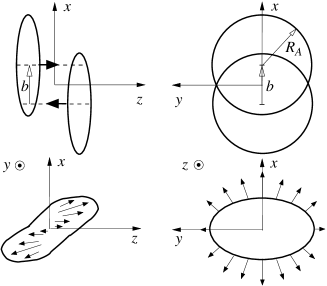
Figure 1: Illustration of a non-central heavy-ion collision with impact parameter $\vec{b}$. The global angular momentum of the produced dense matter is along $-\hat{y}$, opposite to the reaction plane.

Let us consider two colliding nuclei with the projectile of beam momentum per nucleon $\vec{p}_{in}$ moving in the direction of the $z$ axis, as illustrated in Fig. 1. The impact parameter $\vec{b}$, defined as the transverse distance of the center of the projectile nucleus from that of the target, is taken to be along the $\hat{x}$-direction. The normal direction $\vec{n}_{b}$ of the reaction plane, given by,

$$\vec{n}_{b}\equiv\vec{p}_{in}\times\vec{b}/|\vec{p}_{in}\times\vec{b}|,$$ (2)

is along $\hat{y}$. For a non-central collision, the two colliding nuclei carry a finite global orbital angular momentum $L_{y}$ along the direction orthogonal to the reaction plane ($-\hat{y}$). How such a global orbital angular momentum is transferred to the final state particles depends on the equation of state (EOS) of the dense matter. At low energies, the final state is expected to be the normal nuclear matter with an EOS of rigid nuclei. A rotating compound nucleus can be formed when the colliding energy is comparable or smaller than the nuclear binding energy. The finite value of the total orbital angular momentum of the non-central collision at such low energies provides a useful tool for the study of the properties of superdeformed nuclei under such rotation Cederwall:1994gz . At high colliding energy at RHIC, the dense matter is expected to be partonic with an EOS of the quark-gluon plasma. Given such a soft EOS, the global orbital angular momentum would probably never lead to the global rotation of the dense matter. Instead, the total angular momentum will be distributed across the overlapped region of nuclear scattering and is manifested in the shear of the longitudinal flow leading to a finite value of local vorticity density. Under such longitudinal fluid shear, a pair of scattering partons will on average carry a finite value of relative orbital angular momentum in the opposite direction to the reaction plane as defined in Eq. (2). According to Ref. Liang:2004ph , quark (or antiquark) will acquire a global polarization after such scatterings through the spin-orbital coupling in QCD.

The magnitude of the total orbital angular momentum $L_{y}$ and the resulting longitudinal fluid shear can both be estimated within the wounded nucleon model of particle production in which the number of produced particles is assumed to be proportional to the number of participant nucleons. The transverse distributions (integrated over $y$) of participant nucleons in each nucleus can be written as,

$$\frac{dN_{\rm part}^{P,T}}{dx}=\int dydz\rho_{A}^{P,T}(x,y,z,b),$$ (3)

in terms of the participant nucleon number density $\rho_{A}^{P,T}(x,y,z,b)$ in nucleus $A$ in the coordinate system defined above. The superscript $P$ or $T$ denotes projectile or target respectively. The total orbital angular momentum $L_{y}$ of the two colliding nuclei can be defined as,

$$L_{y}=-p_{in}\int x\ dx(\frac{dN_{\rm{part}}^{P}}{dx}-\frac{dN_{\rm{part}}^{T}}{dx}).$$ (4)

where $p_{in}$ is the momentum per incident nucleon.

We assume the Woods-Saxon nuclear distribution,

$$f_{WS}^{P,T}(x,y,z,b)=C\left(1+\exp{\frac{\sqrt{(x\mp b/2)^{2}+y^{2}+z^{2}}-R_{A}}{a}}\right)^{-1}\,.$$ (5)

The participant nucleon number density is then

$$\rho_{A,WS}^{P,T}(x,y,z,b)=f_{WS}^{P,T}(x,y,z,b)\left\{1-\exp\left[-\sigma_{NN}\int dzf_{WS}^{T,P}(x,y,z,b)\right]\right\}\,,$$ (6)

where $\sigma_{NN}\approx 42$ mb is the total cross section of nucleon-nucleon scatterings at the RHIC energy, $C$ is the normalization constant and $a$ is the width parameter set to $a=0.54$ fm.

Shown in Fig. 2 as the solid line is the numerical value of $L_{y}$ as a function of $b$ for the Woods-Saxon nuclear distribution. As a comparison, we also plot as the dashed line the $L_{y}$ distribution with a hard-sphere nuclear distribution which was used in Ref. Liang:2004ph . With the hard-sphere nuclear distribution, the participant nucleon density is given by the overlapping area of two hard spheres,

$$\rho_{A,HS}^{P,T}(x,y,z,b)=f_{A,HS}^{P,T}(x,y,z,b)\theta(R_{A}-\sqrt{(x\pm b/2)^{2}+y^{2}+z^{2}}),$$ (7)

and

$$f_{A,HS}^{P,T}(x,y,z,b)=\frac{3A}{4\pi R_{A}^{3}}\theta(R_{A}-\sqrt{(x\mp b/2)^{2}+y^{2}+z^{2}}),$$ (8)

where $R_{A}=1.12A^{1/3}$ is the nuclear radius and $A$ the atomic number. We note that there are significant differences between two nuclear geometry in the total orbital angular momentum $L_{y}$ in the overlapped region of two colliding nuclei. In both cases, the total orbital angular momentum is huge and is of the order of $10^{4}$ at most impact parameters.

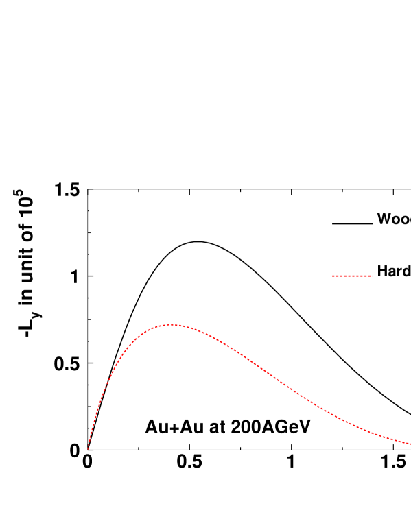
Figure 2: (Color online) The total orbital angular momentum of the overlapping system in $Au+Au$ collisions at the RHIC energy as a function of the impact parameter $b$. The solid and dashed curves are from the Woods-Saxon and hard-sphere distributions, respectively.

Figure 3: The average longitudinal momentum distribution $p_{z}(x,b)$ in unit of $p_{0}=\sqrt{s}/[2c(s)]$ as a function of $x/(R_{A}-b/2)$ for different values of $b/R_{A}$ with the hard sphere (upper panel) and Woods-Saxon (lower panel) nuclear distributions.

Since RHIC data indicate the formation of a strongly coupled quark-gluon plasma Gyulassy:2004zy , we can assume that a partonic system is formed immediately following the initial collision and interactions among partons will lead to both transverse (in $x$-$y$ plane) and longitudinal collective motion in the quark-gluon plasma (QGP). The total orbital angular momentum carried by the produced system will manifest in the longitudinal flow shear or a finite value of the transverse (along $\hat{x}$) gradient of the longitudinal flow velocity. How the total angular momentum is distributed to the longitudinal flow shear and the magnitude of the local relative orbital angular momentum depends on the parton production mechanism and their longitudinal momentum distributions. We consider two different scenarios in this paper: Landau fireball and Bjorken scaling model.

By momentum conservation, the average initial collective longitudinal momentum at any given transverse position can be calculated as the total momentum difference between participating projectile and target nucleons. Since the total multiplicity in $A+A$ collisions is proportional to the number of participant nucleons phobos2 , we can make the same assumption for the produced partons with a proportionality constant $c(s)$ at a given center of mass energy $\sqrt{s}$.

In a Landau fireball model, we assume the produced partons thermalize quickly and have a common longitudinal flow velocity at a given transverse position of the overlapped region. The average collective longitudinal momentum per parton can be written as

$$p_{z}(x,b;\sqrt{s})=p_{0}\frac{dN_{\rm part}^{P}/dx-dN_{\rm part}^{T}/dx}{dN_{\rm part}^{P}/dx+dN_{\rm part}^{T}/dx},$$ (9)

where $p_{0}=\sqrt{s}/[2c(s)]$. The distribution $p_{z}(x,b;\sqrt{s})$ is an odd function in both $x$ and $b$ and therefore vanishes at $x=0$ or $b=0$. In Fig. 3, $p_{z}(x,b;\sqrt{s})$ is plotted as a function of $x$ at different impact parameters $b$. We see that $p_{z}(x,b;\sqrt{s})$ is a monotonically increasing function of $x$ until the edge of the overlapped region $|x\pm b/2|=R_{A}$ beyond which it drops to zero (gradually for Woods-Saxon geometry).

From $p_{z}(x,b;\sqrt{s})$ one can compute the transverse gradient of the average longitudinal collective momentum per parton $dp_{z}/dx$ which is an even function of $x$ and vanishes at $b=0$. One can then estimate the longitudinal momentum difference $\Delta p_{z}$ between two neighboring partons in QGP. On average, the relative orbital angular momentum for two colliding partons separated by $\Delta x$ in the transverse direction is $l_{y}\equiv-(\Delta x)^{2}dp_{z}/dx$. With the hard sphere nuclear distribution, $l_{y}$ is proportional to $dp_{0}/dx\equiv p_{0}/R_{A}=\sqrt{s}/[2c(s)R_{A}]$.

Figure 4: The average orbital angular momentum $l_{y}\equiv-(\Delta x)^{2}dp_{z}/dx$ of two neighboring partons separated by $\Delta x=1$ fm as a function of the scaled transverse coordinate $x/(R_{A}-b/2)$ for different values of the impact parameter $b/R_{A}$ with the hard-sphere (upper panel) and Woods-Saxon (lower panel) nuclear distributions.

In $Au+Au$ collisions at $\sqrt{s}=200$ GeV, the number of charged hadrons per participating nucleon is about 15 phobos2 . Assuming the number of partons per (meson dominated) hadron is about 2, we have $c(s)\simeq 45$ (including neutral hadrons). Given $R_{A}=6.5$ fm, $dp_{0}/dx\simeq 0.34$ GeV/fm and we obtain $l_{0}\equiv-(\Delta x)^{2}dp_{0}/dx\simeq-1.7$ for $\Delta x=1$ fm. In Fig. 4, we show the average local orbital angular momentum $l_{y}$ for two neighboring partons separated by $\Delta x=1$ fm as a function of $x$ for different impact parameter $b$ for both Woods-Saxon and hard-sphere nuclear distributions. We see that $l_{y}$ is in general of the order of 1 and is comparable or larger than the spin of a quark. It is expected that $c(s)$ should depend logarithmically on the colliding energy $\sqrt{s}$, therefore $l_{y}$ should increases with growing $\sqrt{s}$.

In a 3-dimensional expanding system, there could be strong correlation between longitudinal flow velocity and spatial coordinate of the fluid cell. The most simplified picture is the Bjorken scaling scenario Bjorken:1982qr in which the longitudinal flow velocity is identical to the spatial velocity $\eta=\log[(t+z)/(t-z)]$. With such correlation, local interaction and thermalization requires that a parton only interacts with other partons in the same region of longitudinal momentum or rapidity $y$. The width of such region in rapidity is determined by the half-width of the thermal distribution $f(Y,p_{T})=\exp[-p_{T}\cosh(Y-\eta)/T]$ Levai:1994dx , which is approximately $\Delta_{Y}\approx 1.5$ (with $\langle p_{T}\rangle\approx 2T$). The relevant measure of the local relative orbital angular momentum between two interacting partons is, therefore, the difference in parton rapidity distributions at transverse distance of $\delta x\sim 1/\mu$ on the order of the average interaction range.

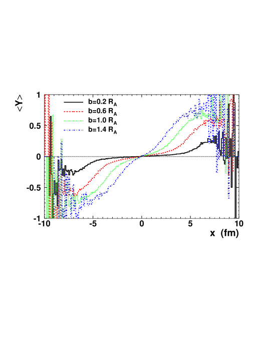
Figure 5: (Color online) The average rapidity $\langle Y\rangle$ of the final state particles as a function of the transverse coordinate $x$ from HIJING Mont Carlo simulations Wang:1991ht ; Wang:1996yf of non-central $Au+Au$ collisions at $\sqrt{s}=200$ GeV.

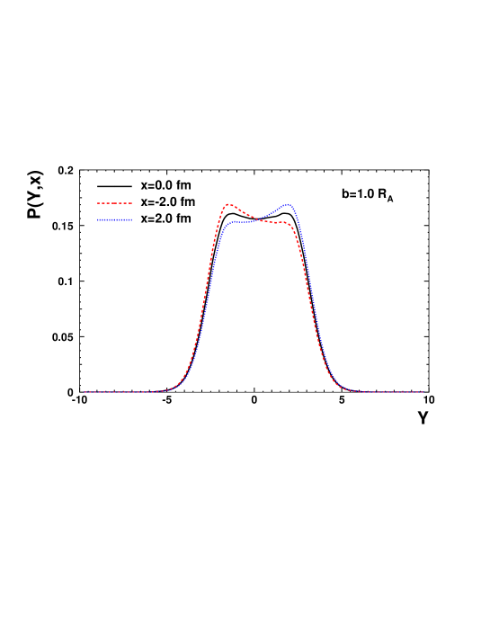
Figure 6: (Color online) The normalized rapidity distribution of particles $P(Y,x)$ [Eq. (10)] at different transverse position $x$ from HIJING simulations of non-central $Au+Au$ collisions at $\sqrt{s}=200$ GeV.

One needs a dynamical model to estimate the local rapidity distributions of produced partons. For such a purpose, we use HIJING Monte Carlo model Wang:1991ht ; Wang:1996yf to calculate the hadron rapidity distributions at different transverse coordinate ($x$) and assume that parton distributions of the dense matter are proportional to the final hadron spectra. Shown in Fig. 5 is the average rapidity $\langle Y\rangle$ as a function of the transverse coordinate $x$ for different values of the impact parameter $b$. The distributions have exactly the same features as given by the wounded nucleon model in Fig. 3. The variation of the rapidity distributions with respect to the transverse coordinate is illustrated in Fig. 6 by the normalized rapidity distributions

$$P(Y,x)=\frac{dN/dxdY}{dN/dx},$$ (10)

at different transverse coordinates, $x=0,\pm 2$ fm. At finite values of the transverse coordinates $x$, the normalized rapidity distributions evidently peak at larger values of rapidity $|Y|$. The shift in the shape of the rapidity distributions will provide the local longitudinal fluid shear or finite relative orbital angular momentum for two interacting partons in the local comoving frame at any given rapidity $Y$. To quantify such longitudinal fluid shear, one can calculate the average rapidity within an interval $\Delta_{Y}$ at $Y$,

$$\langle Y\rangle\approx Y+\frac{\Delta_{Y}^{2}}{12}\frac{1}{P(Y,x)}\frac{\partial P(Y,x)}{\partial Y}.$$ (11)

The average rapidity shear or the difference in average rapidity for two partons separated by a unit of transverse distance $\Delta x=1$ fm is then,

$$\frac{\partial\langle Y\rangle}{\partial x}\approx\frac{\Delta_{Y}^{2}}{12}\frac{\partial^{2}\log P(Y,x)}{\partial Y\partial x}.$$ (12)

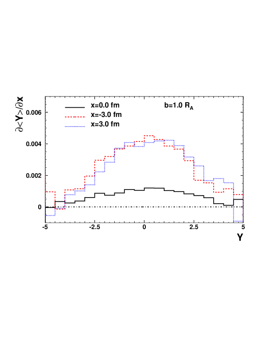
Figure 7: (Color online) The average rapidity shear $\partial\langle Y\rangle/\partial x$ within a window $\Delta_{Y}=1$ as a function of the rapidity $Y$ at different transverse position $x$ from HIJING calculation of non-central $Au+Au$ collisions at $\sqrt{s}=200$ GeV.

Shown in Fig. 7 is the average rapidity shear as a function of the rapidity $y$ at different values of the transverse coordinate $x$ for $\Delta_{Y}=1$. As we can see, the average rapidity shear has a positive and finite value in the central rapidity region. The corresponding local relative longitudinal momentum shear is

$$\frac{\partial\langle p_{z}\rangle}{\partial x}\approx p_{T}\cosh Y\frac{\partial\langle Y\rangle}{\partial x}\,\,.$$ (13)

With $\langle p_{T}\rangle\approx 2T\sim 0.8$ GeV, we have $\partial\langle p_{z}\rangle/\partial x\sim 0.003$ GeV/fm in the central rapidity region of a non-central $Au+Au$ collision at the RHIC energy given by the HIJING simulations, which is much smaller than that from a Landau fireball model estimate.

III Global quark polarization

As we have discussed earlier, under the longitudinal fluid shear, a pair of interacting parton will have a finite value of relative orbital angular momentum along the direction opposite to the reaction plane. In this section, we will calculate quark polarization via scatterings with fixed direction of the relative orbital angular momentum. We will assign a fixed direction of the impact parameter $\vec{x}_{T}$ between two interacting partons to reflect the direction of the relative orbital angular momentum. The magnitude of the relative orbital angular momentum will be charaterized by the relative longitudinal momentum $p$ between two partons separated by a transverse distance $\Delta x\sim 1/\mu$ on the order of the average interaction range. With the averaged longitudinal fluid shear $dp_{z}/dx$ in the center of mass frame of the two colliding nuclei in the Landau fireball model, we have $p=\Delta x(dp_{z}/dx)$. In the Bjorken scaling scenario with strong correlation between spatial and momentum rapidity, the average local longitudinal shear in the comoving frame will be given by $p=\Delta xp_{T}\cosh(Y)\partial\langle Y\rangle/\partial x$, where $p_{T}$ is the average transverse momentum.

III.1 Quark scattering at fixed impact parameter

We consider the scattering $q_{1}(P_{1},\lambda_{1})+q_{2}(P_{2},\lambda_{2})\to q_{1}(P_{3},\lambda_{3})+q_{2}(P_{4},\lambda_{4})$ of two quarks with different flavors, where $P_{i}=(E_{i},\vec{p}_{i})$ and $\lambda_{i}$ in the brackets denote the four momenta and spins of the quarks respectively. The cross section in momentum space is given by,

$$d\sigma_{\lambda_{3}}=\frac{c_{qq}}{F}\frac{1}{4}\sum_{\lambda_{1},\lambda_{2},\lambda_{4}}\mathcal{M}(Q){\mathcal{M}}^{*}(Q)(2\pi)^{4}\delta(P_{1}+P_{2}-P_{3}-P_{4})\frac{d^{3}{\vec{p}}_{3}}{(2\pi)^{3}2E_{3}}\frac{d^{3}{\vec{p}}_{4}}{(2\pi)^{3}2E_{4}},\\$$ (14)

where ${\cal{M}}(Q)$ is the scattering amplitude in momentum space, $Q=P_{3}-P_{1}=P_{2}-P_{4}$ is the four momentum transfer, $c_{qq}=2/9$ is the color factor, and $F=4\sqrt{(P_{1}\cdot P_{2})^{2}-m_{1}^{2}m_{2}^{2}}$ is the flux factor. Since we are interested in the polarization of one of the quarks $q_{1}$ after the scattering, we therefore average over the spins of initial quarks and sum over the spin of the quark $q_{2}$ in the final state.

We work in the center of mass frame of the two quark system. For simplification, we neglect thermal momentum in the transverse direction and assume the relative momentum of the two quarks separated by a transverse distance $\Delta x$ of the order of the effective interaction range $1/\mu$ is simply given by the longitudinal fluid shear.

One can integrate over the final momentum $\vec{p}_{4}$ of the quark $q_{2}$ and the longitudinal component $p_{3z}$ of the quark $q_{1}$, and obtain

$$d\sigma_{\lambda_{3}}=\frac{c_{qq}}{4F}\frac{1}{4}\sum_{\lambda_{1},\lambda_{2},\lambda_{4}}\sum_{i=+,-}\frac{1}{E_{2}|p_{3z}^{i}|+E_{1}|p_{3z}^{i}|}\mathcal{M}(Q_{i}){\mathcal{M}}^{*}(Q_{i})\frac{d^{2}{\vec{q}}_{T}}{(2\pi)^{2}},$$ (15)

where $p_{3z}^{\pm}=\pm\sqrt{p^{2}-{q_{T}}^{2}}$, corresponding to two possible solutions of the energy-momentum conservation in the elastic scattering process, $p=|\vec{p}_{1}|=|\vec{p}_{2}|$; and $\vec{q}_{T}=\vec{p}_{3T}$ is the transverse momentum transfer. For simplicity, we will suppress the summation notation over $i=+,-$ hereafter but keep in mind that the final cross section includes the two terms.

Since we would like to calculate the polarization of one final-state quark with a fixed direction of the orbital angular momentum, or fixed direction of the impact parameter, we will cast the cross section in impact parameter space by making a two dimensional Fourier transformation in the transverse momentum transfer $\vec{q}_{T}$, i.e.,

$$\frac{d^{2}\sigma_{\lambda_{3}}}{d^{2}{\vec{x}}_{T}}=\frac{c_{qq}}{16F}\sum_{\lambda_{1},\lambda_{2},\lambda_{4}}\int\frac{d^{2}{\vec{q}}_{T}}{(2\pi)^{2}}\frac{d^{2}{\vec{k}}_{T}}{(2\pi)^{2}}e^{i({\vec{k}}_{T}-{\vec{q}}_{T})\cdot{\vec{x}}_{T}}\frac{\mathcal{M}({\vec{q}}_{T})}{\Lambda({\vec{q}}_{T})}\frac{{\mathcal{M}}^{*}({\vec{k}}_{T})}{{\Lambda}^{*}({\vec{k}}_{T})},$$ (16)

where ${\mathcal{M}}({\vec{q}}_{T})$ and ${\mathcal{M}}({\vec{k}}_{T})$ are the scattering matrix elements in momentum space with four momentum transfer $Q=(0,\vec{q})$ and $K=(0,\vec{k})$ respectively, and

$$\Lambda({\vec{q}}_{T})=\sqrt{(E_{1}+E_{2})|p_{3z}^{+}|}.$$ (17)

To calculate the quark-quark scattering amplitude in a thermal medium, we will use Hard Thermal Loop (HTL) resummed gluon propagator WELD82 ; hw96 ,

$$\Delta^{\mu\nu}(Q)=\frac{P_{T}^{\mu\nu}}{-Q^{2}+\Pi_{T}(x)}+\frac{P_{L}^{\mu\nu}}{-Q^{2}+\Pi_{L}(x)}+(\alpha-1)\frac{Q^{\mu}Q^{\nu}}{Q^{4}},$$ (18)

where $Q$ denotes the gluon four momentum and $\alpha$ is the gauge fixing parameter. The longitudinal and transverse projectors $P_{T,L}^{\mu\nu}$ are defined by

$${P}_{L}^{\mu\nu} = \frac{-1}{Q^{2}q^{2}}(\omega Q^{\mu}-Q^{2}U^{\mu})(\omega Q^{\nu}-Q^{2}U^{\nu})\,,$$ (19)

$$P_{T}^{\mu\nu} = \tilde{g}^{\mu\nu}+\frac{\tilde{Q}^{\mu}\tilde{Q}^{\nu}}{q^{2}}\,,$$ (20)

with $\omega=Q\!\cdot\!U$, $\tilde{Q}_{\mu}=Q_{\mu}-U_{\mu}\omega$, $q^{2}=-\tilde{Q}^{2}$, $\tilde{g}_{\mu\nu}=g_{\mu\nu}-U_{\mu}U_{\nu}$. Here $U$ is the fluid velocity of the local medium. The transverse and longitudinal self-energies are given by WELD82

$$\Pi_{L}(x) = \mu_{D}^{2}\left[1-\frac{x}{2}\ln\left(\frac{1+x}{1-x}\right)+i\frac{\pi}{2}x\right](1-x^{2})\,,$$ (21)

$$\Pi_{T}(x) = \mu_{D}^{2}\left[\frac{x^{2}}{2}+\frac{x}{4}(1-x^{2})\ln\left(\frac{1+x}{1-x}\right)-i\frac{\pi}{4}x(1-x^{2})\right]$$ (22)

where $x=\omega/q$ and $\mu_{D}^{2}=g^{2}(N_{c}+N_{f}/2)T^{2}/3$ is the Debye screening mass.

With the above HTL gluon propagator, the quark-quark scattering amplitudes can be expressed as

$$\mathcal{M}({\vec{q}}_{T})={\overline{u}}_{{\lambda}_{3}}(P_{1}+Q){\gamma}_{\mu}u_{{\lambda}_{1}}(P_{1}){\Delta}^{\mu\nu}(Q){\overline{u}}_{{\lambda}_{4}}(P_{2}-Q){\gamma}_{\nu}u_{{\lambda}_{2}}(P_{2}),$$ (23)

$${\mathcal{M}}^{*}({\vec{k}}_{T})={\overline{u}}_{{\lambda}_{1}}(P_{1}){\gamma}_{\alpha}u_{{\lambda}_{3}}(P_{1}+K){\Delta}^{\alpha\beta*}(K){\overline{u}}_{{\lambda}_{2}}(P_{2}){\gamma}_{\beta}u_{{\lambda}_{4}}(P_{2}-K).$$ (24)

The product ${\cal{M}}({\vec{q}}_{T}){\cal{M^{*}}}({\vec{k}}_{T})$ can be converted to the following trace form,

$$\sum_{\lambda_{1},\lambda_{2}}{\cal{M}}({\vec{q}}_{T}){\cal{M^{*}}}({\vec{k}}_{T}) = \Delta^{\mu\nu}(Q)\Delta^{\alpha\beta*}(K){\rm Tr}[u_{\lambda_{3}}(P_{1}+K)\bar{u}_{\lambda_{3}}(P_{1}+Q)\gamma_{\mu}(P_{1}/+m_{1})\gamma_{\alpha}]$$ (25)

$$\times{\rm Tr}[u_{\lambda_{4}}(P_{2}-K)\bar{u}_{\lambda_{4}}(P_{2}-Q)\gamma_{\nu}(P_{2}/+m_{2})\gamma_{\beta}].$$

In calculations of transport coefficients such as jet energy loss parameter screen and thermalization time hw96 which generally involve cross sections weighted with transverse momentum transfer, the imaginary part of the HTL propagator in the magnetic sector is enough to regularize the infrared behavior of the transport cross sections. However, in our following calculation of quark polarization, total parton scattering cross section is involved. The contribution from the magnetic part of the interaction has therefore infrared divergence which can only be regularized through the introduction of non-perturbative magnetic screening mass $\mu_{m}\approx 0.255\sqrt{N_{c}/2}g^{2}T$ TBBM93 .

Since we have neglected the thermal momentum perpendicular to the longitudinal flow, the energy transfer $\omega=0$ in the center of mass frame of the two colliding partons. This corresponds to setting $x=0$ in the HTL resummed gluon propagator in Eq. (18). In this case, the center of mass frame of scattering quarks coincides with the local comoving frame of QGP and the fluid velocity is $U^{\mu}=(1,0,0,0)$. The corresponding HTL effective gluon propagator in Feynman gauge that contributes to the scattering amplitudes is reduced to,

$${\Delta}^{\mu\nu}(Q)=\frac{g^{\mu\nu}-U^{\mu}U^{\nu}}{q^{2}+\mu_{m}^{2}}+\frac{U^{\mu}U^{\nu}}{q^{2}+{{\mu}_{D}}^{2}}.$$ (26)

The differential cross section can in general be decomposed into a spin-independent and a spin-dependent part,

$$\frac{d^{2}\sigma_{\lambda_{3}}}{d^{2}{\vec{x}}_{T}}=\frac{d\sigma}{d^{2}{\vec{x}}_{T}}+\lambda_{3}\frac{d\Delta\sigma}{d^{2}{\vec{x}}_{T}}.$$ (27)

with

$$\frac{d^{2}\sigma}{d^{2}{\vec{x}}_{T}}=\frac{1}{2}\left(\frac{d\sigma_{+}}{d^{2}{\vec{x}}_{T}}+\frac{d\sigma_{-}}{d^{2}{\vec{x}}_{T}}\right),$$ (28)

$$\frac{d^{2}\Delta\sigma}{d^{2}{\vec{x}}_{T}}=\frac{1}{2}\left(\frac{d\sigma_{+}}{d^{2}{\vec{x}}_{T}}-\frac{d\sigma_{-}}{d^{2}{\vec{x}}_{T}}\right).$$ (29)

The spin-dependent part will mostly determine the polarization of the final state quark $q_{1}$ via the scattering. The calculation is involved. A simple estimate was given in Ref. Liang:2004ph , using a screened static potential model and small angle approximation. In this case, the cross sections can be written in a general form as,

$$\frac{d^{2}\sigma}{d^{2}{\vec{x}}_{T}} = F(x_{T},E),$$ (30)

$$\frac{d^{2}\Delta\sigma}{d^{2}{\vec{x}}_{T}} = \vec{n}\cdot({\vec{x}}_{T}\times{\vec{p}}\ )\Delta F(x_{T},E),$$ (31)

where $\vec{n}$ is the polarization vector for $q_{1}$ in its rest frame. $F(x_{T},E)$ and $\Delta F(x_{T},E)$ are functions of both $x_{T}\equiv|\vec{x}_{T}|$ and the c.m. energy $E$ of the two quarks. We can show that the quark-quark scattering with HTL propagators has the same form as that in the static potential model Liang:2004ph . But the detailed expressions of $F(x_{T},\hat{s})$ and $\Delta F(x_{T},\hat{s})$ are much more complicated.

In fact, one can show that these two parts of the cross sections should have the same form as given in Eqs. (30) and (31) due to parity conservation in the scattering process. We note that in an unpolarized reaction, the cross section should be independent of any transverse direction. Hence $d\sigma/d^{2}\vec{x}_{T}$ depends only on the magnitude of $x_{T}$ but not on the direction. For the spin-dependent part, the only scalar that we can construct from the available vectors is $\vec{n}\cdot(\vec{p}\times\vec{x}_{T})$.

We note that, $\vec{x}_{T}\times\vec{p}$ is nothing but the relative orbital angular momentum of the two-quark system, $\vec{l}=\vec{x}_{T}\times\vec{p}$. Therefore, the polarized cross section takes its maximum when $\vec{n}$ is parallel or antiparallel to the relative orbital angular momentum, depending on whether $\Delta F$ is positive or negative. This corresponds to quark polarization in the direction $\vec{l}$ or $-\vec{l}$.

As discussed in the last section, the average relative orbital angular momentum $\vec{l}$ of two scattering quarks is in the opposite direction of the reaction plane in non-central $A+A$ collisions. Since a given direction of $\vec{l}$ corresponds to a given direction of $\vec{x}_{T}$, there should be a preferred direction of $\vec{x}_{T}$ at a given direction of the nucleus-nucleus impact parameter $\vec{b}$. The distribution of $\vec{x}_{T}$ at given $\vec{b}$ depends on the collective longitudinal momentum distribution shown in the last section. For simplicity, we consider a uniform distribution of $\vec{x}_{T}$ in all possible directions in the upper half $xy$-plane with $x>0$. In this case, we need to integrate $d\Delta\sigma/d^{2}\vec{x}_{T}$ and $d\sigma/d^{2}\vec{x}_{T}$ over the half plane above $y$-axis to obtain the average cross section at a given $\vec{b}$, i.e.,

$$\sigma = \int_{0}^{+\infty}dx\int_{-\infty}^{+\infty}dy\quad\frac{d^{2}\sigma}{d^{2}{\vec{x}}_{T}},$$ (32)

$$\Delta\sigma = \int_{0}^{+\infty}dx\int_{-\infty}^{+\infty}dy\quad\frac{d^{2}\Delta\sigma}{d^{2}{\vec{x}}_{T}}.$$ (33)

The polarization of the quark is then obtained as,

$$P_{q}=\frac{\Delta\sigma}{\sigma}.$$ (34)

III.2 Small angle approximation

We only consider light quarks and neglect their masses. Carrying out the traces in Eq.(25), we can obtain the expression of the cross section with HTL gluon propagators. The results are much more complicated than those as obtained in Ref.Liang:2004ph using a static potential model. However, if we use small angle or small transverse momentum transfer approximation, the results are still very simple. In this case, with $q_{z}\sim 0$ and $q_{T}\equiv|\vec{q}_{T}|\ll p$, we obtain the spin-independent (unpolarized) cross section ,

$$\frac{d^{2}\sigma}{d^{2}{\vec{x}}_{T}}=\frac{g^{4}c_{qq}}{8}\int\frac{d^{2}{\vec{q}}_{T}}{(2\pi)^{2}}\frac{d^{2}{\vec{k}}_{T}}{(2\pi)^{2}}e^{i({\vec{k}}_{T}-{\vec{q}}_{T})\cdot\vec{x}_{T}}(\frac{1}{q_{T}^{2}+\mu_{m}^{2}}+\frac{1}{q_{T}^{2}+\mu_{D}^{2}})(\frac{1}{k_{T}^{2}+\mu_{m}^{2}}+\frac{1}{k_{T}^{2}+\mu_{D}^{2}}),$$ (35)

and the spin-dependent differential (polarized) cross section,

$$\frac{d^{2}\Delta{\sigma}}{d^{2}{\vec{x}}_{T}} = -i\frac{g^{4}c_{qq}}{16}\int\frac{d^{2}{\vec{q}}_{T}}{(2\pi)^{2}}\frac{d^{2}{\vec{k}}_{T}}{(2\pi)^{2}}e^{i(\vec{k}_{T}-\vec{q}_{T})\cdot\vec{x}_{T}}\frac{(\vec{k}_{T}-\vec{q}_{T})\cdot(\vec{p}\times\vec{n})}{p^{2}}$$ (36)

$$\times(\frac{1}{q_{T}^{2}+\mu_{m}^{2}}+\frac{1}{q_{T}^{2}+\mu_{D}^{2}})(\frac{1}{k_{T}^{2}+\mu_{m}^{2}}+\frac{1}{k_{T}^{2}+\mu_{D}^{2}}).$$

We note that the polarized differential cross can be related to the unpolarized one by,

$$\frac{d^{2}\Delta\sigma}{d^{2}{\vec{x}}_{T}}=-\frac{1}{2{p^{2}}}(\vec{p}\times\vec{n})\cdot\vec{\nabla}_{T}\frac{d^{2}\sigma}{d^{2}{\vec{x}}_{T}}.$$ (37)

Completing the integration over the transverse momentum transfer,

$$\int\frac{d^{2}\vec{q}_{T}}{(2\pi)^{2}}\frac{e^{i\vec{q}_{T}\cdot\vec{x}_{T}}}{q_{T}^{2}+\mu_{m}^{2}}=\int\frac{q_{T}dq_{T}}{2\pi}\frac{J_{0}(q_{T}x_{T})}{q_{T}^{2}+\mu_{m}^{2}},$$ (38)

$$\int_{0}^{\infty}q_{T}dq_{T}\frac{J_{0}(q_{T}x_{T})}{q_{T}^{2}+\mu_{m}^{2}}=K_{0}(\mu_{m}x_{T}),$$ (39)

where $J_{0}$ and $K_{0}$ are the Bessel and modified Bessel functions respectively, we obtain,

$$\frac{d^{2}\sigma}{d^{2}{\vec{x}}_{T}}=\frac{c_{qq}}{2}\alpha_{s}^{2}[K_{0}(\mu_{m}x_{T})+K_{0}(\mu_{D}x_{T})]^{2},$$ (40)

$$\frac{d^{2}\Delta\sigma}{d^{2}{\vec{x}}_{T}}=\frac{c_{qq}\alpha_{s}^{2}}{2}\frac{(\vec{p}\times\vec{n})\cdot\hat{x}_{T}}{p^{2}}[K_{0}(\mu_{m}x_{T})+K_{0}(\mu_{D}x_{T})][\mu_{m}K_{1}(\mu_{m}x_{T})+\mu_{D}K_{1}(\mu_{D}x_{T})],$$ (41)

where $\hat{x}_{T}=\vec{x}_{T}/x_{T}$ is the unit vector of $\vec{x}_{T}$. We compare the above results with that in the screened static potential model (SPM) where one also made the small angle approximation,

$$\Bigl{[}\frac{d\sigma}{d^{2}{\vec{x}}_{T}}\Bigr{]}_{SPM} = \frac{g^{4}c_{T}}{4}\int\frac{d^{2}{\vec{q}}_{T}}{(2\pi)^{2}}\frac{d^{2}{\vec{k}}_{T}}{(2\pi)^{2}}e^{i({\vec{k}}_{T}-{\vec{q}}_{T})\cdot\vec{x}_{T}}\frac{1}{q_{T}^{2}+\mu_{D}^{2}}\frac{1}{k_{T}^{2}+\mu_{D}^{2}},$$ (42)

$$\Bigl{[}\frac{d\Delta{\sigma}}{d^{2}{\vec{x}}_{T}}\Bigr{]}_{SPM} = -i\frac{g^{4}c_{T}}{8}\int\frac{d^{2}{\vec{q}}_{T}}{(2\pi)^{2}}\frac{d^{2}{\vec{k}}_{T}}{(2\pi)^{2}}e^{i(\vec{k}_{T}-\vec{q}_{T})\cdot\vec{x}_{T}}\frac{(\vec{k}_{T}-\vec{q}_{T})\cdot(\vec{p}\times\vec{n})}{p^{2}(q_{T}^{2}+\mu_{D}^{2})(k_{T}^{2}+\mu_{D}^{2})}.$$ (43)

We see that the only difference between the two results is the additional contributions from magnetic gluons, whose contributions are absent in the static potential model. Using Eqs. (38) and (39), we recover the results in Ref. Liang:2004ph ,

$$\Bigl{[}\frac{d\sigma}{d^{2}{\vec{x}}_{T}}\Bigr{]}_{SPM}=\alpha_{s}^{2}c_{T}K_{0}^{2}(\mu_{D}x_{T}),$$ (44)

$$\Bigl{[}\frac{d\Delta\sigma}{d^{2}{\vec{x}}_{T}}\Bigr{]}_{SPM}=\alpha_{s}^{2}c_{T}\frac{(\vec{p}\times\vec{n})\cdot\hat{\vec{x}}_{T}}{p^{2}}\mu_{D}K_{0}(\mu_{D}x_{T})K_{1}(\mu_{D}x_{T})).$$ (45)

III.3 Beyond small angle approximation

Now we present the complete results for the cross-section in impact parameter space using HTL gluon propagators without small angle approximation. The unpolarized and polarized cross section can be expressed in general as,

$$\frac{d\sigma}{d^{2}{\vec{x}}_{T}}=\frac{g^{4}c_{qq}}{64p^{2}}\int\frac{d^{2}{\vec{q}}_{T}}{(2\pi)^{2}}\frac{d^{2}{\vec{k}}_{T}}{(2\pi)^{2}}e^{i({\vec{k}}_{T}-{\vec{q}}_{T})\cdot\vec{x}_{T}}\frac{f(\vec{q}_{T},\vec{k}_{T})}{\Lambda(\vec{q}_{T})\Lambda(\vec{k}_{T})},$$ (46)

$$\frac{d\Delta{\sigma}}{d^{2}{\vec{x}}_{T}}=-i\frac{g^{4}c_{qq}}{64p^{3}}\int\frac{d^{2}{\vec{q}}_{T}}{(2\pi)^{2}}\frac{d^{2}{\vec{k}}_{T}}{(2\pi)^{2}}e^{i(\vec{k}_{T}-\vec{q}_{T})\cdot\vec{x}_{T}}\frac{\Delta f(\vec{q}_{T},\vec{k}_{T})}{\Lambda(\vec{q}_{T})\Lambda(\vec{k}_{T})},$$ (47)

where the kinematic factor becomes $\Lambda(\vec{q}_{T})=\sqrt{2p|p_{3z}^{+}|}$; $f$ and $\Delta f$ are given by,

$$f({\vec{q}}_{T},{\vec{k}}_{T}) = \frac{A_{mm}({\vec{q}}_{T},{\vec{k}}_{T})}{(q^{2}+\mu_{m}^{2})(k^{2}+\mu_{m}^{2})}+\frac{A_{ee}({\vec{q}}_{T},{\vec{k}}_{T})}{(q^{2}+\mu_{D}^{2})(k^{2}+\mu_{D}^{2})}$$ (48)

$$+\frac{A_{me}({\vec{q}}_{T},{\vec{k}}_{T})}{(q^{2}+\mu_{m}^{2})(k^{2}+\mu_{D}^{2})}+\frac{A_{me}({\vec{k}}_{T},{\vec{q}}_{T})}{(q^{2}+\mu_{D}^{2})(k^{2}+\mu_{m}^{2})};$$

$$\Delta f({\vec{q}}_{T},{\vec{k}}_{T}) = \frac{\Delta A_{mm}({\vec{q}}_{T},{\vec{k}}_{T})}{(q^{2}+\mu_{m}^{2})(k^{2}+\mu_{m}^{2})}+\frac{\Delta A_{ee}({\vec{q}}_{T},{\vec{k}}_{T})}{(q^{2}+\mu_{D}^{2})(k^{2}+\mu_{D}^{2})}$$ (49)

$$+\frac{\Delta A_{me}({\vec{q}}_{T},{\vec{k}}_{T})}{(q^{2}+\mu_{m}^{2})(k^{2}+\mu_{D}^{2})}-\frac{\Delta A_{me}({\vec{k}}_{T},{\vec{q}}_{T})}{(q^{2}+\mu_{D}^{2})(k^{2}+\mu_{m}^{2})},$$

$$A_{mm}({\vec{q}}_{T},{\vec{k}}_{T}) = (\vec{q}\cdot\vec{k})^{2}+8p^{2}(\vec{q}\cdot\vec{k})+8p^{3}(q_{z}+k_{z})+16p^{4};$$ (50)

$$A_{ee}({\vec{q}}_{T},{\vec{k}}_{T}) = A_{mm}({\vec{q}}_{T},{\vec{k}}_{T})+4p(q_{z}+k_{z})[(\vec{q}\cdot\vec{k})+p(q_{z}+k_{z})+2p^{2}];$$ (51)

$$A_{me}({\vec{q}}_{T},{\vec{k}}_{T}) = A_{mm}({\vec{q}}_{T},{\vec{k}}_{T})+[-2q_{z}k_{z}(\vec{q}\cdot\vec{k})+4pk_{z}(\vec{q}\cdot\vec{k})-2pq_{z}^{2}k_{z}$$ (52)

$$-2pq_{z}{k_{z}}^{2}+4p^{2}{k_{z}}^{2}+8p^{3}k_{z})];$$

$$\Delta A_{mm}({\vec{q}}_{T},{\vec{k}}_{T}) = -\{[\vec{q}\cdot\vec{k}+4p^{2}-2p(q_{z}+k_{z})](k_{z}\vec{q}_{T}-q_{z}\vec{k}_{T})$$ (53)

$$+2p(\vec{q}\cdot\vec{k}+4p^{2})(\vec{q}_{T}-\vec{k}_{T})\}\cdot(\vec{p}\times\vec{n});$$

$$\Delta A_{ee}({\vec{q}}_{T},{\vec{k}}_{T}) = \Delta A_{mm}({\vec{q}}_{T},{\vec{k}}_{T})-4p(q_{z}+k_{z})[(k_{z}\vec{q}_{T}-q_{z}\vec{k}_{T})-p(\vec{k}_{T}-\vec{q}_{T})]\cdot(\hat{p}\times\vec{n});\phantom{XX}$$ (54)

$$\Delta A_{me}({\vec{q}}_{T},{\vec{k}}_{T}) = \Delta A_{mm}({\vec{q}}_{T},{\vec{k}}_{T})+2pk_{z}[2p(\vec{k}_{T}-\vec{q}_{T})+(q_{z}-k_{z}){\vec{q}}_{T}$$ (55)

$$-(k_{z}\vec{q}_{T}-q_{z}\vec{k}_{T})]\cdot(\hat{p}\times\vec{n})+2q_{z}k_{z}(k_{z}\vec{q}_{T}-q_{z}\vec{k}_{T})\cdot(\hat{p}\times\vec{n}),$$

where $p\equiv|\vec{p}|$. It is useful to note that

$$A_{mm}(\vec{q}_{T},\vec{k}_{T})=A_{mm}(\vec{k}_{T},\vec{q}_{T}),$$ (56)

$$A_{ee}(\vec{q}_{T},\vec{k}_{T})=A_{ee}(\vec{k}_{T},\vec{q}_{T}).$$ (57)

Hence, $f(\vec{q}_{T},\vec{k}_{T})$ is symmetric in its two variables

$$f(\vec{q}_{T},\vec{k}_{T})=f(\vec{k}_{T},\vec{q}_{T}).$$ (58)

Similarly from

$$\Delta A_{mm}(\vec{q}_{T},\vec{k}_{T})=-\Delta A_{mm}(\vec{k}_{T},\vec{q}_{T}),$$ (59)

$$\Delta A_{ee}(\vec{q}_{T},\vec{k}_{T})=-\Delta A_{ee}(\vec{k}_{T},\vec{q}_{T}),$$ (60)

we know that $\Delta f(\vec{q}_{T},\vec{k}_{T})$ is anti-symmetric,

$$\Delta f(\vec{q}_{T},\vec{k}_{T})=-\Delta f(\vec{k}_{T},\vec{q}_{T}).$$ (61)

As mentioned above, to get the average polarization for a fixed direction of the reaction plane in heavy-ion collisions, we need to average over the distribution of $\vec{x}_{T}$. For this purpose, we take the approach as in Ref. Liang:2004ph , and integrate $d\sigma/d^{2}\vec{x}_{T}$ and $d\Delta\sigma/d^{2}\vec{x}_{T}$ over the half plane above the $y$-axis as shown in Eqs. (32) and (33). It is convenient to carry out first the integration over $x$ and $y$ then that over $\vec{q}_{T}$ and $\vec{k}_{T}$. To do this, we use the identity,

$$2\int_{0}^{+\infty}\frac{dx}{2\pi}\int_{-\infty}^{+\infty}\frac{dy}{2\pi}e^{i({\vec{k}}_{T}-{\vec{q}}_{T})\cdot\vec{x}_{T}}=\delta^{2}(\vec{k}_{T}-\vec{q}_{T})+\frac{i}{\pi}\delta(k_{y}-q_{y})\mathcal{P}\frac{1}{k_{x}-q_{x}},$$ (62)

where $\mathcal{P}$ denotes the principal value.

It is useful to note that $\delta^{2}(\vec{k}_{T}-\vec{q}_{T})=\delta^{2}(\vec{q}_{T}-\vec{k}_{T})$ and $\mathcal{P}\frac{1}{k_{x}-q_{x}}=-\mathcal{P}\frac{1}{q_{x}-k_{x}}$. Therefore, only the first term on the r.h.s. of Eq. (62) contributes to the total unpolarized cross section,

$$\sigma=\frac{g^{4}c_{qq}}{64p^{2}}\frac{1}{2}\int_{q_{T}\leq p}\frac{d^{2}{\vec{q}}_{T}}{(2\pi)^{2}}\frac{f(\vec{q}_{T},\vec{q}_{T})}{\Lambda^{2}(\vec{q}_{T})}.$$ (63)

The polarized cross section $\Delta\sigma$ receives contribution only from the second term,

$$\Delta{\sigma}=\frac{g^{4}c_{qq}}{64p^{3}}\int_{-p}^{p}\frac{dq_{y}}{2\pi}\int_{-\sqrt{p^{2}-{q_{y}}^{2}}}^{\sqrt{p^{2}-{q_{y}}^{2}}}\frac{dq_{x}}{2\pi}\int_{-\sqrt{p^{2}-{q_{y}}^{2}}}^{\sqrt{p^{2}-{q_{y}}^{2}}}\frac{dk_{x}}{2\pi}\frac{1}{k_{x}-q_{x}}\frac{\Delta f(q_{x},q_{y};k_{x},q_{y})}{\Lambda(\vec{q}_{T})\Lambda(\vec{k}_{T})}.$$ (64)

Changing the integration variable $q_{T}=p\sin\theta$ and $\xi=\sin^{2}(\theta/2)$ in the expression of the total cross section $\sigma$, we obtain,

$$\sigma=\frac{\pi c_{qq}\alpha_{s}^{2}}{4\hat{s}}\int_{0}^{1}d\xi\left\{\frac{1+\xi^{2}}{(\xi+\beta_{m}\tilde{T}^{2})^{2}}+\frac{(1-\xi)^{2}}{(\xi+\beta_{D}\tilde{T}^{2})^{2}}+\frac{2(1-\xi)}{(\xi+\beta_{D}\tilde{T}^{2})(\xi+\beta_{m}\tilde{T}^{2})}\right\},$$ (65)

where $\beta_{D}=(\mu_{D}/T)^{2}=4\pi\alpha_{s}(N_{c}+N_{f}/2)/3$, $\beta_{m}=(\mu_{m}/T)^{2}=0.255^{2}(4\pi)^{2}\alpha_{s}^{2}N_{c}/2$, and $\tilde{T}=T/\sqrt{\hat{s}}$ with $\sqrt{\hat{s}}$ the center of mass energy of the $qq$-system. The integration can be carried out analytically,

$$\sigma = \frac{\pi c_{qq}\alpha_{s}^{2}}{4\hat{s}}\left\{4+\frac{1}{\beta_{m}\tilde{T}^{2}}+\frac{1}{\beta_{D}\tilde{T}^{2}}-\frac{2}{1+\beta_{m}\tilde{T}^{2}}-2(\beta_{m}\tilde{T}^{2}+\frac{1+\beta_{m}\tilde{T}^{2}}{\beta_{m}\tilde{T}^{2}-\beta_{D}\tilde{T}^{2}})\ln(1+\frac{1}{\beta_{m}\tilde{T}^{2}})\right.$$ (66)

$$\left.-2(\beta_{D}\tilde{T}^{2}+\frac{\beta_{m}\tilde{T}^{2}-2\beta_{D}\tilde{T}^{2}-1}{\beta_{m}\tilde{T}^{2}-\beta_{D}\tilde{T}^{2}})\ln(1+\frac{1}{\beta_{D}\tilde{T}^{2}})\right\}.$$

Similarly, we make the variable substitutions $q_{y}=p\sqrt{1-t^{2}}$, $q_{x}=pt\sqrt{1-\xi^{2}}$, $k_{x}=pt\sqrt{1-\eta^{2}}$ in the integration for $\Delta{\sigma}$ and obtain,

$$\Delta\sigma =-\frac{c_{qq}\alpha_{s}^{2}}{8\pi\hat{s}}\int_{-1}^{1}dt\int_{0}^{1}d\xi\int_{0}^{1}d\eta\frac{t^{2}\sqrt{\xi\eta}}{\sqrt{1-t^{2}}\sqrt{1-\xi^{2}}\sqrt{1-\eta^{2}}}$$ (67)

$$\times\left\{\frac{(1-t^{2})(4+t\xi+t\eta)-2(t^{2}\xi\eta+1)+2t(1+\xi\eta)(5+t^{2}\xi\eta)/(\xi+\eta)}{(1-t\xi+2\beta_{m}\tilde{T}^{2})(1-t\eta+2\beta_{m}\tilde{T}^{2})}\right.$$

$$\ \ \ \left.+\frac{(1-t^{2})(t\xi+t\eta)+2(t^{2}\xi\eta+1)+2t(1+\xi\eta)(1+t^{2}\xi\eta)/(\xi+\eta)}{(1-t\xi+2\beta_{D}\tilde{T}^{2})(1-t\eta+2\beta_{D}\tilde{T}^{2})}\right.$$

$$\ \ \ \left.+\frac{2(1-t^{2})(2+t\xi+t\eta)+8t(1+\xi\eta)(1+t\eta)/(\xi+\eta)}{(1-t\xi+2\beta_{m}\tilde{T}^{2})(1-t\eta+2\beta_{D}\tilde{T}^{2})}\right\}.$$

Note that in the calculation of both the polarized and unpolarized cross sections we have limited the range of integration over the transverse momentum due to energy conservation. Such restriction is not imposed in the small angle approximation in Ref. Liang:2004ph . We see that, at given $\beta_{m}$ and $\beta_{D}$, both $\sigma$ and $\Delta\sigma$ are functions of the variable $\tilde{T}=T/\sqrt{\hat{s}}$. Since $\beta_{m}$ and $\beta_{D}$ depend on $\alpha_{s}$, the polarization $P_{q}=\Delta\sigma/\sigma$ also depends on the value of $\alpha_{s}$.

We can now carry out the integration numerically to get the quark polarization $P_{q}$. Before we show the numerical results, it is useful to look at two limits.

(1) High energy limit. At very high energies, $\sqrt{\hat{s}}\gg T$ or $\tilde{T}\ll 1$, we have,

$$\sigma=\frac{\pi c_{qq}\alpha_{s}^{2}}{4\hat{s}\tilde{T}^{2}}\left\{\frac{1}{(1+4\beta_{m}\tilde{T}^{2})\beta_{m}}+\frac{1}{(1+4\beta_{D}\tilde{T}^{2})\beta_{D}}+\frac{2}{\beta_{D}-\beta_{m}}\ln\frac{\beta_{D}(1+4\beta_{m}\tilde{T}^{2})}{\beta_{m}(1+4\beta_{D}\tilde{T}^{2})}\right\},$$ (68)

$$\Delta\sigma=-\frac{4c_{qq}\alpha_{s}^{2}}{\pi\hat{s}}\int_{0}^{1}dt\left[\frac{1}{\sqrt{t^{2}+4\beta_{m}\tilde{T}^{2}}}\tan^{-1}{\sqrt{\frac{1-t^{2}}{t^{2}+4\beta_{m}\tilde{T}^{2}}}}+\frac{1}{\sqrt{t^{2}+4\beta_{D}\tilde{T}^{2}}}\tan^{-1}{\sqrt{\frac{1-t^{2}}{t^{2}+4\beta_{D}\tilde{T}^{2}}}}\right]^{2}.$$ (69)

This is the case where the small angle approximation can be made. The above can also be obtained from Eqs. (35-36) given in the last section by carrying out the integration over $\vec{x}_{T}$ in the half plane of $x>0$.

(2) Low energy limit. In the limit $\sqrt{\hat{s}}\ll T$, we have $q_{T}^{2}+\mu_{D}^{2}\approx\mu_{D}^{2}$ and $q_{T}^{2}+\mu_{m}^{2}\approx\mu_{m}^{2}$, the cross sections become

$$\sigma = \frac{c_{qq}\alpha_{s}^{2}}{8\hat{s}}\pi(\frac{\sqrt{\hat{s}}}{T})^{4}\left(\frac{8}{3\beta_{m}^{2}}+\frac{2}{3\beta_{D}^{2}}+\frac{2}{\beta_{m}\beta_{D}}\right),$$ (70)

$$\Delta\sigma = -\frac{c_{qq}\alpha_{s}^{2}}{16\pi\hat{s}}(\frac{\sqrt{\hat{s}}}{T})^{4}\left[-\frac{1}{\beta_{m}^{2}}\left(\frac{1}{192}\Gamma^{4}(\frac{1}{4})+\frac{1}{2}\Gamma^{4}(\frac{3}{4})\right)+\frac{1}{\beta_{D}^{2}}\left(\frac{1}{192}\Gamma^{4}(\frac{1}{4})+\Gamma^{4}(\frac{3}{4})\right)\right.$$ (71)

$$\left.+\frac{2}{\beta_{m}\beta_{D}}\left(\frac{1}{192}\Gamma^{4}(\frac{1}{4})+\Gamma^{4}(\frac{3}{4})\right)\right].$$

Given the corresponding values of the $\Gamma$-function, one can obtain numerically,

$$\Delta\sigma\approx-\frac{c_{qq}\alpha_{s}^{2}}{16\pi\hat{s}}(\frac{\sqrt{\hat{s}}}{T})^{4}\left(-\frac{2.03}{\beta_{m}^{2}}+\frac{3.15}{\beta_{D}^{2}}+\frac{6.30}{\beta_{m}\beta_{D}}\right).$$ (72)

We see that in the low energy limit the magnetic part contributes with different sign from the electric one. The polarization $P_{q}=\Delta\sigma/\sigma$ is given by

$$P_{q}\approx-\frac{3}{2\pi^{2}}\frac{-2.03\beta_{D}^{2}+3.15\beta_{m}^{2}+6.30\beta_{m}\beta_{D}}{8\beta_{D}^{2}+2\beta_{m}^{2}+6\beta_{m}\beta_{D}},$$ (73)

which tends to be a constant in this low energy limit. In the weak coupling limit $\alpha_{s}\ll 1$, $\beta_{D}\gg\beta_{m}$ the above constant $P_{q}\approx 0.04$ is a small positive number.

It is also interesting to look at the contributions from the electric part only. The corresponding cross sections, denoted with subscription $E$, are

$$\left(\frac{d\sigma}{d^{2}{\vec{x}}_{T}}\right)_{E}=\frac{g^{4}c_{qq}}{64p^{2}}\int\frac{d^{2}{\vec{q}}_{T}}{(2\pi)^{2}}\frac{d^{2}{\vec{k}}_{T}}{(2\pi)^{2}}\frac{A_{ee}({\vec{q}}_{T},{\vec{k}}_{T})e^{i({\vec{k}}_{T}-{\vec{q}}_{T})\cdot\vec{x}_{T}}}{\Lambda(\vec{q}_{T})\Lambda(\vec{k}_{T})(q^{2}+\mu_{D}^{2})(k^{2}+\mu_{D}^{2})},$$ (74)

$$\left(\frac{d\Delta{\sigma}}{d^{2}{\vec{x}}_{T}}\right)_{E}=-i\frac{g^{4}c_{qq}}{64p^{3}}\int\frac{d^{2}{\vec{q}}_{T}}{(2\pi)^{2}}\frac{d^{2}{\vec{k}}_{T}}{(2\pi)^{2}}\frac{\Delta A_{ee}({\vec{q}}_{T},{\vec{k}}_{T})e^{i(\vec{k}_{T}-\vec{q}_{T})\cdot\vec{x}_{T}}}{\Lambda(\vec{q}_{T})\Lambda(\vec{k}_{T})(q^{2}+\mu_{D}^{2})(k^{2}+\mu_{D}^{2})}.$$ (75)

Carrying out the integration over $d^{2}\vec{x}_{T}$ in the half plane with $x>0$, we obtain,

$$\sigma_{E}=\frac{\pi c_{qq}\alpha_{s}^{2}}{4\hat{s}}\int_{0}^{1}\frac{(1-\xi)^{2}d\xi}{(\xi+\beta_{D}\tilde{T}^{2})^{2}}=\frac{\pi c_{qq}\alpha_{s}^{2}}{4\hat{s}}\left[2+\frac{1}{\beta_{D}\tilde{T}^{2}}-2(1+\beta_{D}\tilde{T}^{2})\ln(1+\frac{1}{\beta_{D}\tilde{T}^{2}})\right],$$ (76)

$$\Delta\sigma_{E} =-\frac{c_{qq}\alpha_{s}^{2}}{8\pi\hat{s}}\int_{-1}^{1}dt\int_{0}^{1}d\xi\int_{0}^{1}d\eta\frac{t^{2}\sqrt{\xi\eta}}{\sqrt{1-t^{2}}\sqrt{1-\xi^{2}}\sqrt{1-\eta^{2}}}$$ (77)

$$\times\left\{\frac{(1-t^{2})(t\xi+t\eta)+2(t^{2}\xi\eta+1)+2t(1+\xi\eta)(1+t^{2}\xi\eta)/(\xi+\eta)}{(1-t\xi+2\beta_{D}\tilde{T}^{2})(1-t\eta+2\beta_{D}\tilde{T}^{2})}\right\}.$$

In the high energy limit, where small angle approximation is applicable, we have,

$$\sigma_{E} = \frac{\pi c_{qq}\alpha_{s}^{2}}{4\hat{s}\beta_{D}\tilde{T}^{2}(1+4\beta_{D}\tilde{T}^{2})},$$ (78)

$$\Delta\sigma_{E} = -\frac{4c_{qq}\alpha_{s}^{2}}{\pi\hat{s}}\int_{0}^{1}\frac{dt}{t^{2}+4\beta_{D}\tilde{T}^{2}}\left[\tan^{-1}{\sqrt{\frac{1-t^{2}}{t^{2}+4\beta_{D}\tilde{T}^{2}}}}\ \right]^{2}.$$ (79)

In the low energy limit, we have,

$$\sigma_{E} = \frac{c_{qq}\alpha_{s}^{2}}{12\hat{s}\beta_{D}^{2}}\pi(\frac{\sqrt{\hat{s}}}{T})^{4},$$ (80)

$$\Delta\sigma_{E} = -\frac{c_{qq}\alpha_{s}^{2}}{16\pi\hat{s}}(\frac{\sqrt{\hat{s}}}{T})^{4}\frac{1}{\beta_{D}^{2}}\left(\frac{1}{192}\Gamma^{4}(\frac{1}{4})+\Gamma^{4}(\frac{3}{4})\right).$$ (81)

The polarization in this case,

$$P_{q}^{E}\equiv{\Delta\sigma_{E}}/{\sigma_{E}}=-\frac{3}{4\pi^{2}}\left(\frac{1}{192}\Gamma^{4}(\frac{1}{4})+\Gamma^{4}(\frac{3}{4})\right)\approx-0.24$$ (82)

is a negative constant which can also be obtained from Eq. (73) by taking the limit $\beta_{m}\gg\beta_{D}$.

III.4 Numerical results

We now carry out the integration in Eq. (67) numerically and obtain the results for the quark polarization at intermediate energies between the high-energy and low-energy limit. The results are shown in Fig. 8 as functions of $\sqrt{\hat{s}}/T$. The quark polarization ($-P_{q}$) along the reaction plane approaches a small negative value as we have shown in the last subsection in the low-energy limit. The value of the low energy limit varies with $\alpha_{s}$ as given by Eq. (73). Such a dependence on $\alpha_{s}$ is a consequence of the magnetic and electric screening masses in the polarized and unpolarized cross sections which have different dependence on $\alpha_{s}$. However, from Eq. (73), the low-energy limit of the quark polarization becomes independent of $\alpha_{s}$ in the weak coupling limit $\alpha_{s}\rightarrow 0$ when $\beta_{m}\ll\beta_{D}$.

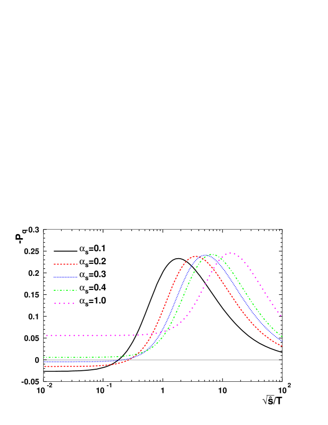
Figure 8: (Color online) Quark polarization -$P_{q}$ as a function of $\sqrt{\hat{s}}/T$ for different $\alpha_{s}$’s.

As one increases the relative c.m. energy, the quark polarization changes drastically with $\sqrt{\hat{s}}/T$. It increases to some maximum values and then decreases with the growing energy, approaching the result of small angle approximation in the high-energy limit. This structure is caused by the interpolation between the high-energy and low-energy behavior dominated by the magnetic part of the interaction in the weak coupling limit $\alpha_{s}<1$. Therefore, the position of the maxima in $\sqrt{\hat{s}}$ should approximately scale with the magnetic mass $\mu_{m}$. This is indeed the case as shown in Fig. 9.

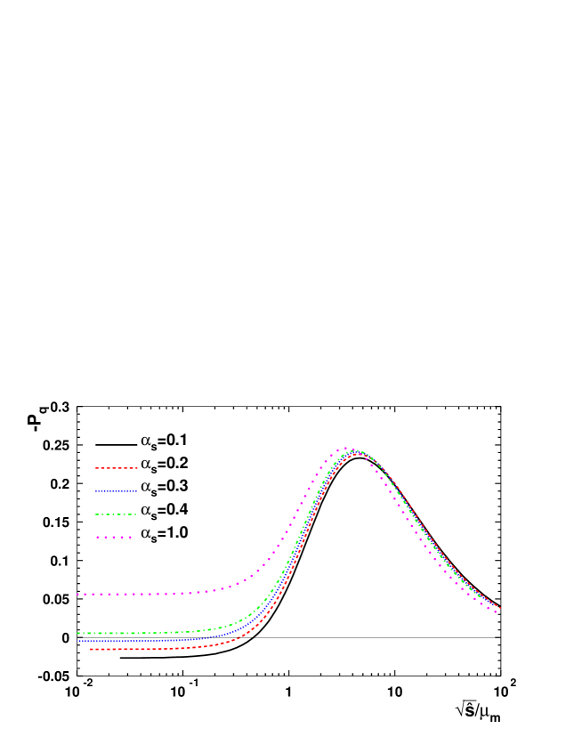
Figure 9: (Color online) Quark polarization -$P_{q}$ as a function of $\sqrt{\hat{s}}/\mu_{m}$ for different values of $\alpha_{s}$.

To further understand the interpolation between the high and low-energy limits in the numerical results, we also compare them in Fig. 10 with the results with the electric gluon exchange only. Without the contribution from the magnetic gluon interaction, the quark polarization takes a relatively large value $P_{q}\approx-0.24$ at low energies and then decreases with $\sqrt{\hat{s}}$ at high energies. The magnetic interaction in the low-energy limit apparently has a different sign in the contribution to the polarized cross section relative to that of the electric one. The net polarization is therefore reduced at finite $\alpha_{s}$ to smaller negative values when $\alpha_{s}\ll 1$. The electric contribution to the net quark polarization also corresponds to the limit $\mu_{m}\gg\mu_{D}$ or $\alpha_{s}\gg 1$ in the full result. Even though our perturbative approach is no longer valid in such a limit, it indicates that the net quark polarization remains a finite negative value in the strong coupling limit as shown in Fig. 9.

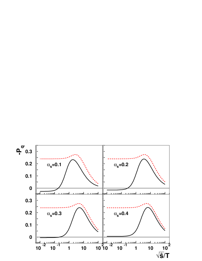
Figure 10: (Color online) Quark polarization -$P_{q}$ as a function of $\sqrt{\hat{s}}/T$ with the full HTL gluon propagator (solid) as compared to the results with the electric part of the interaction only (dashed).

In Fig. 11 we also compare the full numerical results (solid lines) with those of the small angle approximation in the high-energy limit (dashed lines) as given by Eqs. (68) and (69). These two groups of results indeed agree with each other at high energies. However, they both are different from the results of the static potential model in the small angle limit (dotted lines) Liang:2004xn which does not have the energy conservation restriction in the integration over the transverse momentum transfer.

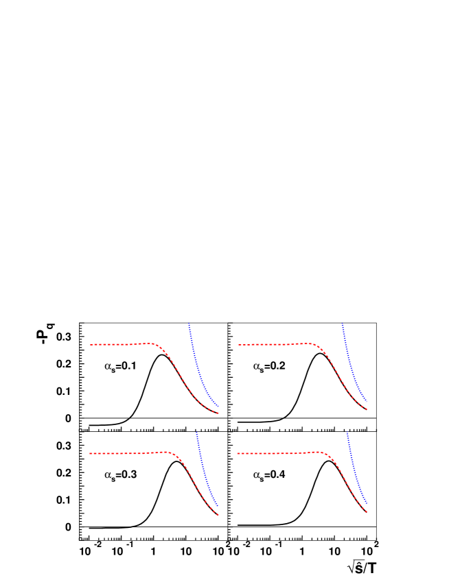
Figure 11: (Color online) Comparison of the results obtained using HTL gluon propagator (solid line) with those under small angle approximation (dashed line) and those using the screened static potential model under small angle approximation (dotted line).

IV Conclusions and discussions

In this paper, we have extended an earlier study Liang:2004xn of the global quark polarization caused by the longitudinal fluid shear in non-central heavy-ion collisions. We have calculated the average local relative orbital angular momentum or longitudinal fluid shear with two extreme models: Landau fireball and Bjorken scaling model. In the Landau fireball model, we assumed a wounded nucleon model for local particle production with both the hard-sphere and Woods-Saxon nuclear distributions. Each parton is then assumed to carry an average longitudinal flow velocity calculated from the net longitudinal momentum at a given transverse position. In the Bjorken scaling model we considered correlation between spatial and momentum rapidity in a 3-dimensional expanding system for which we calculated the average rapidity or longitudinal momentum shear (derivative of the average rapidity or the longitudinal momentum) with respect to the transverse position $x$. The shear determines the local relative orbital angular momentum in the comoving frame at a given rapidity. These two model calculations provide estimates of the local fluid shear in two extreme limits.

We have also extended the calculation of the global quark polarization $P_{q}$ within perturbative QCD at finite temperature beyond the small angle approximation of the previous study Liang:2004xn which might not be valid for small values of the local longitudinal fluid shear or the average c.m. energy $\sqrt{\hat{s}}$ of a colliding quark pair. We found that the magnetic part of the interaction in one-gluon exchange is particularly important at low energies which cancels the contribution from the electric interaction and leads to smaller negative values of the net quark polarization in the weak coupling limit ($\alpha_{s}<1$). The final global quark polarization therefore is small in both the low and high-energy limits. It can, however, reach a peak value of about $P_{q}\approx-0.24$ at an energy determined by the nonperturbative magnetic mass $\sqrt{\hat{s}}\sim 4\mu_{m}\approx g^{2}T\sqrt{N_{c}/2}$. For $\sqrt{\hat{s}}<\mu_{m}$, the average quark polarization becomes significantly smaller.

In semi-peripheral $Au+Au$ collisions ($b=R_{A}$) at the RHIC energy, one can assume an average temperature $T\approx 400$ MeV Muller:2005en . With $\alpha_{s}\approx 0.3$, the global quark polarization reaches its peak value at c.m. energy about 1.8 GeV. Since the magnetic interaction dominates the quark-quark interaction in our calculation, we can assume that the average interaction range in the transverse direction is given by the magnetic mass, $\Delta x\sim 1/\mu_{m}$. According to our estimates of the longitudinal fluid shear, the average c.m. energy of the quark pair under such fluid shear is $\sqrt{\hat{s}}\sim 0.8~{}{\rm GeV}^{2}/\mu_{m}\approx 0.17$ GeV (from Fig. 4) in the Landau fireball model. In the Bjorken scaling model (from Fig. 7), the c.m. energy provided by the local fluid shear is $\sqrt{\hat{s}}\sim 0.004\langle p_{T}\rangle\cosh(y)~{}{\rm fm}^{-1}/\mu_{m}\approx 0.001$ GeV in the central rapidity region (we assume $\langle p_{T}\rangle\sim 2T$). In both cases, the longitudinal fluid shear is so weak that the global quark polarization due to perturbative quark-quark scatterings is quite small according to our numerical calculations that go beyond the small angle approximation.

In heavy-ion collisions at the Large Hadron Collider (LHC) energy $\sqrt{s}=5.5$ TeV, the average multiplicity density per participant nucleon pair was estimated to be about a factor of 3 larger than that at the RHIC energy Li:2001xa . The corresponding longitudinal fluid shear and the average c.m. energy of a quark pair will be about a factor 6 larger than that at the RHIC energy in the Landau fireball model, assuming the temperature is about 1.44 higher. One can also expect the average local longitudinal fluid shear in the Bjorken scenario at LHC is similarly amplified compared to the RHIC energy in particular at large rapidity. Therefore, the resulting net quark polarization should also be larger at LHC.

We want to emphasize that the above numerical estimate is based on a perturbative calculation via quark-quark scatterings in the weak coupling limit. It is still possible that quarks could acquire large global polarization through interaction in the strong coupling limit, as hinted by our results with large values of the strong coupling constant even though such a perturbative approach becomes invalid. The finite value of the quark polarization could be detected via measurements of the global hyperon polarization or the vector meson spin alignment with respect to the reaction plane. According to our estimate of the longitudinal fluid shear, the effect is more significant at large rapidity under the Bjorken scenario of the initial parton production.

In the limit of vanishing local orbital angular momentum provided by the longitudinal fluid shear, the approach we used in this paper in the impact-parameter representation might not be valid anymore. However, the final spin-polarization due to the spin-orbital interaction should approach to zero in this limit, which is approximately the result of our full calculation.

V Acknowledgment

The authors thank B. Muller for pointing out the scenario of Bjorken scaling model of initial parton production and J. Deng for his help in the numerical calculation of the local orbital angular momentum with the Woods-Saxon geometry. This work was supported in part by National Natural Science Foundation of China (NSFC) under No. 10525523; the startup grant from University of Science and Technology of China (USTC) in association with 100 talents project of Chinese Academy of Sciences (CAS) and by NSFC grant No. 10675109 and, the Director, Office of Energy Research, Office of High Energy and Nuclear Physics, Divisions of Nuclear Physics, of the U.S. Department of Energy under No. DE-AC03-76SF00098.

References

• (1) M. Gyulassy and L. McLerran, Nucl. Phys.  A 750, 30 (2005) [arXiv:nucl-th/0405013].
• (2) P. Jacobs and X. N. Wang, Prog. Part. Nucl. Phys.  54, 443 (2005) [arXiv:hep-ph/0405125].
• (3) K. H. Ackermann et al. [STAR Collaboration], Phys. Rev. Lett.  86, 402 (2001) [arXiv:nucl-ex/0009011].
• (4) D. Teaney, Phys. Rev.  C 68, 034913 (2003) [arXiv:nucl-th/0301099].
• (5) A. Majumder, B. Muller and X. N. Wang, arXiv:hep-ph/0703082.
• (6) A. Adil and M. Gyulassy, Phys. Rev.  C 72, 034907 (2005) [arXiv:nucl-th/0505004]; A. Adil, M. Gyulassy and T. Hirano, Phys. Rev.  D 73, 074006 (2006) [arXiv:nucl-th/0509064].
• (7) Z. T. Liang and X. N. Wang, Phys. Rev. Lett. 94, 102301 (2005), arXiv:nucl-th/0410079, Erratum 96, 039901 (E) (2006).
• (8) B. Betz, M. Gyulassy and G. Torrieri, arXiv:0708.0035 [nucl-th].
• (9) Z. T. Liang and X. N. Wang, Phys. Lett. B 629, 20 (2005) [arXiv:nucl-th/0411101].
• (10) I. Selyuzhenkov [STAR Collaboration], AIP Conf. Proc.  870, 712 (2006) [arXiv:nucl-ex/0608034].
• (11) I. Selyuzhenkov [STAR Collaboration], J. Phys. G 32, S557 (2006) [arXiv:nucl-ex/0605035].
• (12) I. Selyuzhenkov [STAR Collaboration], talk given at the 19th International Conference on Ultra-Relativistic Nucleus-Nucleus Collisions (QM2006), November 14-20, 2006, Shanghai, China.
• (13) J.H. Chen [STAR Collaboration], talk given at the 19th International Conference on Ultra-Relativistic Nucleus-Nucleus Collisions (QM2006), November 14-20, 2006, Shanghai, China.
• (14) I. Selyuzhenkov [STAR Collaboration], talk given at the International Workshop on Hadron Physics and Property of High Baryon Density Matter, November 22-25, 2006, Xi’An, China.
• (15) Z.B. Tang [STAR Collaboration], talk given at the International Workshop on Hadron Physics and Property of High Baryon Density Matter, November 22-25, 2006, Xi’An, China.
• (16) B. I. Abelev et al. [STAR Collaboration], arXiv:0705.1691 [nucl-ex].
• (17) B. Cederwall et al., Phys. Rev. Lett.  72, 3150 (1994).
• (18) B. B. Back et al. [PHOBOS Collaboration], arXiv:nucl-ex/0301017; R. Nouicer et al. [PHOBOS Collaboration], J. Phys. G 30, S1133 (2004).
• (19) J. D. Bjorken, Phys. Rev.  D 27, 140 (1983).
• (20) P. Levai, B. Muller and X. N. Wang, Phys. Rev.  C 51, 3326 (1995) [arXiv:hep-ph/9412352].
• (21) X. N. Wang and M. Gyulassy, Phys. Rev.  D 44, 3501 (1991).
• (22) X. N. Wang, Phys. Rept.  280, 287 (1997) [arXiv:hep-ph/9605214].
• (23) H. A. Weldon, Phys. Rev. D 26, 1394 (1982).
• (24) X.-N. Wang, Phys. Lett. B485,157 (2000).
• (25) H. Heiselberg and X.-N. Wang, Nucl Phys. B462, 389 (1996).
• (26) T. S. Biró and B. Müller, Nucl. Phys. A561, 477 (1993).
• (27) B. Muller and K. Rajagopal, Eur. Phys. J.  C 43, 15 (2005) [arXiv:hep-ph/0502174].
• (28) S. Y. Li and X. N. Wang, Phys. Lett.  B 527, 85 (2002) [arXiv:nucl-th/0110075].