Status reports from the GRACE Group

Abstract

We discuss a new approach for the numerical evaluation of loop integrals. The fully numerical calculations of an infrared one-loop vertex and a box diagram are demonstrated. To perform these calculations, we apply an extrapolation method based on the $\epsilon$-algorithm. In our approach, the super high precision control in the numerical manipulation is essential to handle the infrared singularity. We adopt a multi-precision library named HMLib for the precision control in the calculations.

1 Introduction

Measurements of fundamental parameters with high precision will be one of the important issues at the ILC experiment. We suppose to determine the masses and couplings for the standard model (SM) and some of the beyond the standard models like the minimal supersymmetric model(MSSM) within a few percent precision [1]. These precision measurements require the knowledge of high precision theoretical predictions, especially the computation of higher loop corrections. Since,the vast number of Feynman diagrams appear in the loop calculations, performing such computation is absolutely beyond the human power if it should be done by hand. The procedure of a perturbation calculation is well established, thus computers must be able to take the place of human hand. In this purpose several groups have developed computer programs which generate Feynman diagrams and calculate cross sections automatically, like GRACE [2], FeynArts-FormCalc [3] and CompHEP [4].

The GRACE system, developed by Minamitateya group, is one of the systems to calculate Feynman amplitudes including loop diagrams. Our final goal of the GRACE system is to construct the fully automatic computation system of multi-loop integrals. In this stage, it is successfully working for one-loop calculations in both the SM [5] and the MSSM [6]. However, the fully automatic way to compute multi-loop integrals is not established, thus the system is still semi-automatic. Especially, since infrared singularities require the analytic manipulations, it makes difficult to handle the singularity in the automatic way. To avoid such a difficulty, we really need to treat loop integrals in a fully numerical way.

In this paper, we discuss the fully numerical computation of one-loop integrals with existing infrared singularities. First, we demonstrate the calculations of an one-loop vertex and a box diagram in QED case. We put a fictitious photon mass as a regulator of the infrared singularities. For the calculations, we adopt the very brute force way as the numerical extrapolation method. In our approach, the $\epsilon$-algorithm is efficient. We also introduce a precision control technique to handle the numerical calculation with extremely small photon masses.

In QCD, one can not avoid to use the dimensional regularization to treat the infrared singularity. The sector decomposition technique [7] is useful to pick up the singularities but in general, the numerical integration of each term is not trivial because the denominators of the integrands can be zero in the integral region. Therefore, the extrapolation method should be effective in this case, too.

The layout of this paper is as follows. In section 2, we show the basic idea and formula of the loop integrals. Numerical results of the infrared one-loop vertex and box diagram are shown in section 3. The case for the dimensional regularization is discussed in section 4. In section 5 we will summarize this paper.

$\lambda$ [GeV] Average lost-bits Maximum lost-bits $10^{-20}$ 88 92 $10^{-21}$ 98 102 $10^{-22}$ 108 112

Table 1: Lost-bits information from HMLib with the quadruple precision arithmetic. $\lambda$ is a fictitious photon mass.

2 Basic idea

The basic idea of our numerical method is the combination of an efficient multi-dimensional integration routine and an extrapolation method. Here, we consider a scalar one-loop n-point integral given by

$${I}(\epsilon)=\int\frac{d^{4}l}{(2\pi)^{4}i}\frac{1}{(l^{2}-m_{1}^{2}+i\epsilon)((l+p_{1})^{2}-m_{2}^{2}+i\epsilon)\cdots((l+\sum_{j=1}^{n-1}p_{j})^{2}-m_{n}^{2}+i\epsilon)},$$ (1)

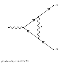
Figure 1: One-loop vertex diagram

where $l$ is the loop momentum, $p_{j}$ is the momentum of the $j$th external particle and $m_{j}$ is the mass carried by the $j$th internal line. Putting $\epsilon>0$ in the denominator of Feynman integrals to prevent the integral from diverging, we can get the numerical results of ${I}(\epsilon)$ for a given $\epsilon$. Calculating a sequence of ${I}(\epsilon_{l})$ with various value of $\epsilon_{l}=\epsilon_{0}\times(const.)^{-l}$ $(l=0,1,2,\cdots)$ and extrapolating into the limit of $\epsilon\rightarrow 0$, we can get the final result of the integration which appears in a physical amplitude.

In this approach, we use DQAGE routine in the multi-dimensional integration. It is included in the package QUADPACK [8] and it is a globally adaptive integration routine. We also apply the $\epsilon$-algorithm introduced by P.Wynn[9]. The algorithm accelerates the conversion of the sequences. Our approach is very efficient for massive one-loop and two-loop integrals including non-scalar type integrals [10, 11, 12, 13].

In the above massive cases, the results are consistent with analytic ones very well, even in the double precision arithmetic or quadruple precision arithmetic. On the other hand, for massless cases, we need much more careful treatments to handle the infrared singularities. For the infrared divergent diagram, it becomes harder to get a result with an enough accuracy even in the quadruple precision arithmetic. Thus, the precision control of the numerical integration becomes another important elements in our approach [14].

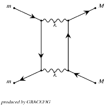
Figure 2: One-loop box diagram in QED

For the precision control, we use HMlib[15] as the multi-precision library. The advantage of this library is that it gives an information of the lost-bits during the calculation, thus we can guarantee the precision of the results. In Table 1, we show an example of the lost-bits information supplied by HMLib. Here, we demonstrated the calculation of one-loop vertex diagram (Fig.1). The diagram includes the infrared singularity due to the photon exchange. We put a fictitious photon mass $\lambda$ as a regulator of the infrared singularity. In P-precision presentation implemented in HMlib, a sign bit is 1 bit and an exponent bit is 15 bits and a mantissa is ($32\times P-16$) bits with based on IEEE754 FP. When $P=4$ (quadruple precision), the mantissa becomes 112 bits. In the Table when $\lambda$ is $10^{-23}$ GeV, the maximum number of lost-bits is the same as the number of bits of the mantissa. This means quadruple-precision is not enough and we have to perform the calculation within octuple or higher precision.

3 Numerical results

For the one-loop vertex diagram shown in Fig. 1, the loop integral we consider in this paper is

$$I=\int_{0}^{1}dx\int_{0}^{1-x}dy{\frac{1}{D}},$$ (2)

where

$$D=-xys+{(x+y)}^{2}m^{2}+(1-x-y)\lambda^{2}.$$ (3)

Here $s$ denotes squared central mass energy and $m$ and $\lambda$ are a mass of external particles and a fictitious photon mass respectively. Replacing $s$ by $s+i\epsilon$ in (3) and applying extrapolation method, we obtain the numerical results which are shown in Table 2 [14]. Results are compared to analytic results evaluated by the formula in [16]. The combination of the extrapolation method and multi precision control with HMLib works very well and we get stable results even though the photon mass becomes much smaller as $10^{-160}$ GeV.

$n$ Numerical Results P Analytical Results [P=4] -30 -0.150899286980769753D-01 $\pm$ 0.771D-26 8 -0.150899286980482291E-01 0.189229839615898822D-02 $\pm$ 0.124D-25 8 0.189229839615525389E-02 -80 -0.405390396284235075D-01 $\pm$ 0.580D-15 16 -0.405390396283445396E-01 0.478581216125478532D-02 $\pm$ 0.401D-12 16 0.478581216112143981E-02 -120 -0.608983283726997427D-01 $\pm$ 0.556D-15 32 -0.608983283725815879E-01 0.710062317325786663D-02 $\pm$ 0.415D-12 32 0.710062317309438855E-02 -160 -0.812576170752810666D-01 $\pm$ 0.549D-10 32 -0.812576183472699269E-01 0.941543418501223556D-02 $\pm$ 0.109D-11 32 0.941543432496722442E-02

Table 2: Numerical results of the one-loop vertex diagram with $\sqrt{s}=500$ GeV, $t=-150^{2}$ $GeV^{2}$, $m=m_{e}=0.5\times 10^{-3}$ GeV. Photon mas $\lambda=10^{n}$[GeV] and P denotes P-precision. The upper is the result of Real part and the lower is one of Imaginary part.

We also demonstrate the calculation of the one-loop box diagram shown in Fig.2. Here, we consider the following integral,

$$I=\int_{0}^{1}dx\int_{0}^{1-x}dy\int_{0}^{1-x-y}dz{\frac{1}{D^{2}}},$$ (4)

where

$$D = -xys-tz(1-x-y-z)+(x+y)\lambda^{2}$$ (5)

$$+ (1-x-y-z)(1-x-y)m^{2}+z(1-x-y)M^{2}.$$ (6)

$s$ denotes squared central mass energy and $m$ and $M$ are external masses of particles. Again, replacing $s$ by $s+i\epsilon$ in eq.(6) and applying extrapolation method, we obtain the numerical results. We show the real part of the numerical results with the analytic ones in Table 3 as an example [14]. The results are almost consistent each other. However, since high precision computation costs huge CPU time, we only have done the quadruple precision arithmetic. Thus the results are not reliable when the photon mass is smaller as $10^{-30}$ GeV.

4 Dimensional Regularization

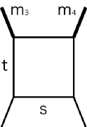
Figure 3: One-loop box diagram with two massive external legs, so called ”hard” case.

We next consider the diagram contains two massive and two massless external legs, and internal lines are all massless with the dimensional regularization, where $D=\varepsilon+2$ (Fig. 3). In order to pick up the singularities, we apply the sector decomposition technique. The loop integral is expressed as follows:

$$I_{4} = \int\prod_{i=1}^{4}dx_{i}{\frac{\delta(1-\sum x_{i})}{(-sx_{1}x_{3}-tx_{2}x_{4}-m_{3}^{2}x_{3}x_{4}-m_{4}^{2}x_{1}x_{4})^{2-\varepsilon}}},$$ (7)

$$= \sum_{n=-2,-1,0,\cdots}C_{n}\times\varepsilon^{n}.$$ (8)

In the case of $s=123$ GeV²,$t=-200$ GeV², $m_{3}^{2}=50$ GeV² and $m_{4}^{2}=60$ GeV², the denominator of each integrand corresponding to $1/\varepsilon$ and the finite term can be zero. Again, $+i\epsilon$ is introduced in the denominator of eq.(8) to specify the analyticity of it and the extrapolation method does work to perform the numerical integration. Table 4 shows the complete numerical integration can reconstruct the results with the analytical expressions [17].

$n$ Numerical Results P Numerical Results [P=4] -15 -0.1927861102670278D-06 $\pm$ 0.314D-14 4,4,2 -0.1927861122439641E-06 -20 -0.2472486348234972D-06 $\pm$ 0.586D-15 4,4,2 -0.2472486352599175E-06 -25 -0.3017111253761463D-06 $\pm$ 0.111D-13 4,4,2 -0.3017111582758710E-06 -30 -0.3562028882831722D-06 $\pm$ 0.867D-10 4,4,2 -0.3561736812918245E-06

Table 3: Numerical results of the loop integral of one-loop box diagram with $\sqrt{s}=500$ GeV, $t$ = -$150^{2}GeV^{2}$, $m$ = 0.5 $\times 10^{-5}$ GeV, $M$ = 150 GeV. Photon mas $\lambda=10^{n}$[GeV] and P denotes P-precision. This is results of Real part.

$n$ Numerical Results Analytic Results -2 -0.40650406505E-04 -0.40650406504E-04 -1 -0.34156307031E-03 -0.34156306995E-03 0 -0.14929502492E-02 -0.14929502456E-02

Table 4: Numerical v.s. Analytical results in the double precision arithmetic. Real part of $C_{n}$ of Fig. 3 with $s$ = 123 GeV², $t$ = -200 GeV², $m_{3}^{2}$ = 50 GeV² and $m_{4}^{2}$=60 GeV².

5 Summary

We discussed a new approach of the numerical method for multi-loop integrals. The combination of an efficient multi-dimensional integration routine and an extrapolation method is applicable to the one-loop integral even though it includes infrared singularities both with the introduction of the fictitious mass and the dimensional regularization. We demonstrated the fully numerical calculations for one-loop vertex and box diagram with infrared singularities. To handle the infrared singularities, high precision control is essential and in some case quadruple precision is not enough to obtain the stable results. In our calculations, we applied the multi-precision library HMLib which has the high performance of the precision control . Our method is efficient and we obtain reliable results for one-loop vertex and box diagrams with infrared singularities.

References

-
[1]
see for example,
ILC Reference Design Report volume 2:”Physics at the ILC”,
eds A. Djouadi et al., ILC Global Design Effort and World Wide Study (2007) -
[2]
G. Belanger, F. Boudjema, J. Fujimoto, T. Ishikawa,
T. Kaneko, K. Kato, Y. Shimizu,
Phys.Rept. 430 117 (2006);
J. Fujimoto, T. Ishikawa, M. Jimbo, T. Kaneko, K. Kato, S. Kawabata, T. Kon, M. Kuroda, Y. Kurihara, Y. Shimizu and H. Tanaka, Comput. Phys. Commun. 153 106 (2003); Program package GRACE/SUSY (GRACE v2.2.0) is available from http://minami-home.kek.jp/ . - [3] T. Hahn, Nucl. Phys. Proc. Suppl. 89 231 (2000) ; T. Hahn, Comput. Phys. Commun. 140 418(2001) ; T. Hahn and C. Schappacher, Comput. Phys. Commun. 143 54 (2002).
- [4] A.Pukhov et al., arXiv:hep-ph/9908288; A. Semenov, Nucl. Instrum. Meth. A502 558 (2003).
- [5] F.Boudjema, J.Fujimoto, T.Ishikawa, T.Kaneko, K.Kato, Y.Kurihara, Y.Shimizu, Y.Yasui, Electroweak Corrections for the Study of the Higgs Potential at the LC LCWS05, Stanford (2005).
- [6] J. Fujimoto, T. Ishikawa, M. Jimbo, T. Kon, Y. Kurihara, M. Kuroda, Phys. Rev. D75, 113002 (2007).
- [7] T. Binoth, G. Heinrich, Nucl.Phys. B585, 741 (2000), T. Binoth, G. Heinrich, Nucl.Phys. B680, 375 (2004).
- [8] R. Piessens, E. de Doncker, C. W. Ubelhuber and D. K. Kahaner, QUADPACK, A Subroutine Package for Automatic Integration, Springer Series in Computational Mathematics. Springer-Verlag, (1983).
-
[9]
P.Wynn,
Math. Tables Automat. Computing 10 91(1956):
P.Wynn, SIAM J. Numer. Anal. 3 91(1966). - [10] E. de Doncker, Y. Shimizu, J. Fujimoto and F. Yuasa, Comput. Phys. Commun. 159 145 (2004).
- [11] E. de Doncker, J. Fujimoto and F. Yuasa, Nucl. Instr. and Meth A534 269 (2004).
- [12] E. de Doncker, S. Li, Y. Shimizu, J. Fujimoto and F. Yuasa, Lecture Notes in Computer Science 3514,151 (2005).
-
[13]
E. de Doncker, Y. Shimizu, J. Fujimoto and F. Yuasa,
A talk in LoopFest V, June 19-21, 2006. SLAC, USA,
http://www-conf.slac.stanford.edu/loopfestv/proc/proceedings.htm. - [14] F. Yuasa, E. de Doncker, J. Fujimoto, N. Hamaguchi, T. Ishikawa and Y. Shimizu, Precise Numerical Evaluation of the Scalar One-Loop Integrals with the Infrared Divergence, ACAT workshop, Amsterdam, (2007);arXiv:0709.0777.
-
[15]
N. Hamaguchi,
IPSJ SIG Technical Report 2007-ARC-172 (22)/ 2007-HPC-109 (22) pp. 127-132.
N. Hamaguchi, IPSJ SIG Technical Report 2007-ARC-172 (23)/ 2007-HPC-109 (23) pp. 133-138. - [16] J. Fujimoto, Y. Shimizu, K. Kato and Y. Oyanagi, Progress of Theoretical Physics Vol.87 No. 5 1232 (1992).
- [17] G. Duplani, B. Nii, Eur. Phys. J. C 20, 357 (2001), Y. Kurihara, Eur.Phys. J.C45, 427 (2006).