Interaction and thermodynamics of spinons in the XX chain

Abstract

The mapping between the fermion and spinon compositions of eigenstates in the one-dimensional spin-1/2 $XX$ model on a lattice with $N$ sites is used to describe the spinon interaction from two different perspectives: (i) For finite $N$ the energy of all eigenstates is expressed as a function of spinon momenta and spinon spins, which, in turn, are solutions of a set of Bethe ansatz equations. The latter are the basis of an exact thermodynamic analysis in the spinon representation of the $XX$ model. (ii) For $N\to\infty$ the energy per site of spinon configurations involving any number of spinon orbitals is expressed as a function of reduced variables representing momentum, filling, and magnetization of each orbital. The spins of spinons in a single orbital are found to be coupled in a manner well described by an Ising-like equivalent-neighbor interaction, switching from ferromagnetic to antiferromagnetic as the filling exceeds a critical level. Comparisons are made with results for the Haldane-Shastry model.

1 Introduction

To the few and precious situations, where interacting quantum many-body systems can be analyzed by rigorous methods in great detail, belong a host of models for quantum spin chains. Prominent among them is the $XX$ model for exchange-coupled electron spins on a one-dimensional lattice,

$$\mathcal{H}_{XX}\doteq\sum_{\ell=1}^{N}[S_{\ell}^{x}S_{\ell+1}^{x}+S_{\ell}^{y}S_{\ell+1}^{y}].$$ (1.1)

Periodic boundary conditions are assumed throughout. The $XX$ model is the special case $\Delta=0$ of the $XXZ$ model. The latter also has terms $\Delta S_{\ell}^{z}S_{\ell+1}^{z}$ in its Hamiltonan. The $XXZ$ model is exactly solvable via Bethe ansatz for arbitrary values of $\Delta$ [1, 2].

The composition of all $XX$ eigenstates by free, spinless Jordan-Wigner fermions has been the basis of most advances in the study of the thermodynamics, correlation functions, and dynamics [3, 4, 5, 6, 7, 8, 9, 10, 11, 12, 13, 14, 15]. The alternative composition of the same states provides a framework for the interpretation of dominant features observed in the spectra and intensity distributions of dynamical quantities. Spinons have spin 1/2 and semionic exclusion statistics [16]. The one-to-one mapping between the fermion and spinon compositions was presented in a recent study of the $m$-spinon dynamic structure factors based on product formulas for transition rates [17]. Here we use the fermion-spinon mapping for different purposes.

In preparation of our main themes – interaction and thermodynamics of spinons – we introduce alternative quantum numbers for fermion momenta and for spinon momenta and spins, along with rules that translate the fermion composition of any $XX$ eigenstate into the corresponding spinon composition (Sec. 2). For the energy of an arbitrary $XX$ eigenstate, the mapping converts its dependence on the fermion quantum numbers into its dependence on the spinon quantum numbers. The resulting expression is akin to a coordinate Bethe ansatz (CBA) for the spinon momenta and spins (Sec. 3). From an entirely different perspective, the $XX$ chain is interpreted as a set of interacting spinon orbitals with internal degrees of freedom exhibiting features akin to electrons in partially filled electronic shells (Sec. 4). A thermodynamic Bethe ansatz (TBA) for spinons is constructed from the CBA discussed in Sec. 3 and then analyzed exactly (Sec. 5). Several aspects of spinon interaction and spinon thermodynamics discussed for the $XX$ model are compared with corresponding properties of the Haldane-Shastry (HS) model (A).

2 $XX$ spectrum from top down and bottom up

The complete spectrum of eigenstates of the $XX$ model is described via complementary sets of quasiparticles with different exclusion statistics and with their vacua at opposite ends of the energy range: (i) the free Jordan-Wigner lattice fermions and the closely related partially interacting magnon solutions of the CBA, (ii) the interacting spinons. Only the fermions are free. Therefore, it is desirable to perform calculations in the fermion representation. On the other hand, it is desirable to use the spinons for the interpretation of the spectrum and the dynamics because the ground state (physical vacuum) coincides (for even $N$) with the spinon vacuum. The magnons are important because they are natural products of the CBA, the method on which most advances in the analysis of the $XXZ$ model rest [18].

2.1 Magnons and fermions

The structure of the Bethe ansatz equations (BAE) for the states with magnetization $M_{z}=N/2-r$ of the $XXZ$ model,

$$e^{\imath Nk_{i}}=\prod_{j\neq i}^{r}\left[-\frac{1+e^{\imath(k_{i}+k_{j})}-2\Delta e^{\imath k_{i}}}{1+e^{\imath(k_{i}+k_{j})}-2\Delta e^{\imath k_{j}}}\right],\quad i=1,\ldots,r,$$ (2.1)

undergoes a drastic simplification in the $XX$ limit $\Delta\to 0$:

$$e^{\imath Nk_{i}}=(-1)^{r-1},\quad i=1,\ldots,r,$$ (2.2)

with solutions

$$k_{i}=\pi-\frac{2\pi}{N}I_{i},$$ (2.3)

provided $k_{i}+k_{j}\neq\pi$ holds for all pairs of magnon momenta. The Bethe quantum numbers $I_{i}$ are integers for odd $r$ and half-integers for even $r$ over the range $|I_{i}|\leq N/2$. This simple rule becomes more complicated for $\Delta\neq 0$ [18].

In those instances, where magnon pairs with momenta $k_{i}+k_{j}\to\pi$ exist, the limit $\Delta\to 0$ in (2.1) is singular, and nontrivial solutions exist [19]. The solution of the BAE as a limit process then yields both real and complex-conjugate solutions. The critical magnon pairs do not contribute to the energy of the eigenstate,

$$E=\sum_{i=1}^{r}\cos k_{i}.$$ (2.4)

Thus removing one critical pair from an eigenstate yields a degenerate eigenstate with $\Delta k=\pi$ and $\Delta M_{z}=2$. This kind of degeneracy is predicted and quantitatively described by the $sl_{2}$ loop algebra symmetry for the case $\Delta=0$ [20, 21]. Critical pairs occur only for even $N$. If $N$ is odd the criticality condition for the associated Bethe quantum numbers, $I_{i}+I_{j}=N/2~{}\mathrm{mod}~{}N$, is impossible to satisfy, given that $I_{1},I_{2}$ are either both integers or both half-integers.

The $XX$ Hamiltonian (1.1) can be mapped onto a system of free, spinless lattice fermions by means of the Jordan-Wigner transformation followed by the Fourier transform [3]:

$$\mathcal{H}_{XX}=\sum_{\{p_{i}\}}\cos p_{i}\,c_{p_{i}}^{\dagger}c_{p_{i}},$$ (2.5)

where the sum is over all sets of distinct fermion momenta from the allowed values

$$p_{i}=\frac{\pi}{N}\,\bar{m}_{i},\quad\bar{m}_{i}\in\left\{\begin{tabular}[]{ll}${\displaystyle\{1,3,\ldots,2N-1\}}$&for even $N_{f}$\\ ${\displaystyle\{0,2,\ldots,2N-2\}}$&for odd $N_{f}$\end{tabular}\right..$$ (2.6)

The number of fermions in an eigenstate depends on the magnetization $M_{z}$:

$$N_{f}=\frac{N}{2}-M_{z},\qquad-\frac{N}{2}\leq M_{z}\leq\frac{N}{2}.$$ (2.7)

For even $N$ the ground state of $\mathcal{H}_{XX}$ is unique. It has $M_{z}=0$ and thus contains $N_{f}=N/2$ fermions. For odd $N$ the ground state is fourfold degenerate.

How are the fermions and the magnons, which originate from different methods of analysis, related to one another? It is evident from (2.3) and (2.6) that the non-critical magnons have momenta and energies that exactly correspond to fermion momenta and energies. Whereas the fermions are free, the non-critical magnons are not. They scatter off each other elastically. However, the associated phase shift is $\pi$ for all such events. This reflects the well-known equivalence between hard-core bosons and free fermions in one dimension.

Regarding eigenstates with critical magnon pairs we note that they are at least twofold degenerate within their invariant Hilbert subspace of given quantum numbers $k$ and $M_{z}$. This degeneracy between states with $\Delta k=0$ and $\Delta M_{z}=0$ suggests that the magnon eigenbasis for states with critical pairs is related to the fermion eigenbasis by an orthogonal transformations within the invariant $(k,M_{z})$-subspaces. The critical and non-critical magnons of the $XX$ model can be interpreted as fragments of string excitations in the context of the CBA applied to the $XXZ$ model. The limit $\Delta\to 0$ is singular in the BAE (2.1) but the singularities can be removed by a basis transformation.

One consequence is that the thermodynamics of magnons as analyzed via TBA for the $XXZ$ model becomes equivalent, for $\Delta\to 0$, to the thermodynamics of free fermions [18]. Another consequence is that the advances recently reported in the calculation of transition rates via algebraic Bethe ansatz for the $XXZ$ model [19] can be translated into corresponding advances, for $\Delta\to 0$, in the fermion representation of the $XX$ model [17].

2.2 Spinons

The unique ground state of $\mathcal{H}_{XX}$ for even $N$ coincides with the vacuum for spinon quasiparticles. The total number of spinons is confined to the range $0\leq N_{s}\leq N$ and restricted to be even (odd) if $N$ is even (odd). Knowledge of the numbers of spinons with spin up and spin down determines both $N_{s}$ and $M_{z}$.

$$N_{+}+N_{-}=N_{s},\qquad N_{+}-N_{-}=2M_{z}.$$ (2.8)

The range of momentum values for spinon orbitals was first determined in the context of the HS model [16]. Minor adaptations are necessary for the $XX$ model [17]. The orbitals available for occupation by spinons are equally spaced at $\Delta\kappa=2\pi/N$ and their number is $(N-N_{s})/2+1$, where $N_{s}=0,2,\ldots,N$ for even $N$ and $N_{s}=1,3,\ldots,N$ for odd $N$. The allowed orbital momentum values are

$$\kappa_{i}=\frac{\pi}{N}\,m_{i},\quad m_{i}=\frac{N_{s}}{2},\frac{N_{s}}{2}+2,\ldots,N-\frac{N_{s}}{2}.$$ (2.9)

Each available orbital may be occupied by spinons of either spin orientation without further restrictions. The spinon quantum numbers $m_{i}^{\sigma}$ are thus integers for even $N$ and half-integers for odd $N$. The $XX$ eigenstate specified by spinon quantum numbers $\{m_{i}^{\sigma}\}$ has wave number

$$k=\left(\frac{\pi}{N}\sum_{\sigma=\pm}\sum_{j_{\sigma}=1}^{N_{\sigma}}m_{j_{\sigma}}^{\sigma}-\frac{N\pi}{2}\right)~{}\mathrm{mod}(2\pi).$$ (2.10)

Figure 1: (a) Fermion orbitals available to $N_{f}$ fermions and (b) spinon orbitals available to $N_{s}$ spinons in $XX$ eigenstates for $N=5$. Fermion orbitals can be either vacant (open circle) or singly occupied (full circle). The particular fermion configuration shown in each row represents one lowest energy states for given $N_{f}$. Spinon orbitals can be either vacant or occupied by up to $N_{s}$ spinons with arbitrary spin polarization. No specific spinon configuration is shown.

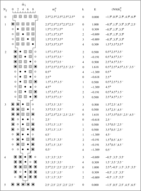
Figure 2: Fermion configurations of all eigenstates for $N=5$. Fermionic particles (holes) are denoted by full (open) circles. Spinon particles with spin up (down) are denoted by squares around open (full) circles. The fermion quantum numbers $\bar{m}_{i}$ can be read off the diagram. The spinon quantum numbers $m_{i}^{\sigma}$ are given explicitly and can be inferred from the fermion configuration as explained in the text. Also given are the wave number $k$ (in units of $2\pi/N$) and the energy $E$ of each $XX$ eigenstate. The spinon momenta $k_{i}^{\sigma}$ are discussed in Sec. 3.2.

In Ref. [17] we demonstrated how to keep track of the spinons in the fermion representation for a system with $N=4$, where the (unique) ground state is the spinon vacuum. Here we consider $N=5$ for illustration, where the ground state consists of four 1-spinon states. The set of allowed fermion momentum states for $N_{f}=0,1,\ldots,5$ is shown in Fig. 1(a) and the sets of allowed spinon momentum states for $N_{s}=1,3,5$ in Fig. 1(b). An expanded version of Fig. 1(a) is shown in Fig. 2 with all $2^{N}=32$ distinct fermion configurations (circles) grouped according to $N_{f}$ and with the associated spinon configurations (squares) indicated. The $\lor$-shaped line of Fig. 1(a) becomes the forked line in Fig. 2.

The exact spinon configuration is encoded in the fermion configuration as described in the following: (i) Consider the $\lor$ or the fork as dividing the fermion momentum space into two domains, the inside and the outside. The outside domain wraps around at the extremes ($\bar{m}_{i}=N$ mod$(N)=0$). (ii) Every fermionic hole (open circle) inside represents a spin-up spinon (square surrounding open circle) and every fermionic particle (full circle) outside represents a spin-down spinon (square surrounding full circle). (iii) Any number of adjacent spinons in the representation of Fig. 2 are in the same orbital of Fig. 1(b). Two spin-up (spin-down) spinons that are separated by $\ell$ consecutive fermionic particles (holes) have quantum numbers separated by $2\ell$. (iv) The spinon quantum numbers are sorted in increasing order from the right-hand prong of the fork toward the left in the inside domain $(m_{i}^{+})$ and toward the right with wrap-around through the outside domain $(m_{i}^{-})$.

3 Interacting spinons

Naturally, the key to studying the spinon interaction for the $XX$ model is the mapping between the fermion composition and the spinon composition of every eigenstate, combined with the fact that the fermions are free. Here we study this interaction on the level of spinon particles, then, in Sec. 4, on the level of spinon orbitals.

3.1 Energy of spinon configurations

Consider an arbitrary eigenstate of $\mathcal{H}_{XX}$ for finite (even or odd) $N$ in the fermion eigenbasis. Given the configuration of fermion quantum numbers $\{\bar{m}_{1},\ldots,\bar{m}_{N_{f}}\}$ of the state selected, the mapping described in Sec. 2.2 produces a unique configuration of spinon quantum numbers with range restricted as in (2.9):

$$\frac{N_{s}}{2}\leq m_{1}^{\sigma}\leq m_{2}^{\sigma}\leq\cdots\leq m_{N_{\sigma}}^{\sigma}\leq N-\frac{N_{s}}{2},\quad\sigma=\pm.$$ (3.1)

Note that we have sorted them into two groups according to spin orientation and, within each group, in ascending order. The number of distinct $m_{i}^{\sigma}$-configurations satisfying (3.1) for fixed $N$ and $N_{s}$ is $(N+1)!/[N_{s}!(N+1-N_{s})!]$. Summation over $N_{s}$ yields $2^{N}$. All eigenstates are accounted for. Their energies are found to have the following dependence on the spinon quantum numbers:

$$E\big{(}\{m_{j_{+}}^{+}\},\{m_{j_{-}}^{-}\}\big{)}=E_{0}(N_{+},N_{-})+\sum_{\sigma=\pm}\,\sum_{j_{\sigma}=1}^{N_{\sigma}}\sin\big{(}\kappa_{j_{\sigma}}^{\sigma}-\tau_{j_{\sigma}}^{\sigma}\big{)}$$ (3.2)

with

$$\kappa_{j_{\sigma}}^{\sigma}=\frac{\pi}{N}\,m_{j_{\sigma}}^{\sigma},\quad\tau_{j_{\sigma}}^{\sigma}=\frac{\pi}{N}\big{(}N_{\sigma}+1-2j_{\sigma}\big{)},\quad\sigma=\pm,$$ (3.3)

and where the reference energy

$$E_{0}(N_{+},N_{-})=\sum_{\{\bar{m}_{i}^{0}\}}\cos\left(\frac{\pi}{N}\,\bar{m}_{i}^{0}\right),$$ (3.4)

$$\{\bar{m}_{i}^{0}\} = \left\{\frac{1}{2}(N+N_{+}-N_{-}+2),\frac{1}{2}(N+N_{+}-N_{-}+6),\ldots\right.$$ (3.5)

$$\hskip 99.58464pt\left.\ldots,\frac{1}{2}(3N-N_{+}+N_{-}-2)\right\},$$

only depends on $N_{+}-N_{-}$, i.e. on $M_{z}$. For even $N$, $E_{0}$ is the energy of the lowest eigenstate for given $M_{z}$, but for odd $N$ it does not represent the energy of any eigenstate.

The spinons are not free, notwithstanding the fact that expression (3.2) is a sum of 1-spinon terms. The spinon interaction is hidden in the sorting criterion (3.1). Moving one spinon into a different orbital will, in general, affect more than just one term in (3.2), and switching the spin of one spinon affects all terms including the reference energy.

3.2 Bethe ansatz equations for spinons

The very structure of Eq. (3.2) exhibits features characteristic of a CBA solution for spinons undergoing two-body elastic scattering. When we employ the spinon quantum numbers (3.1) in the role of Bethe quantum numbers (BQN) for the spinon configuration, Eq. (3.2) can be rewritten in the form

$$E\big{(}\{m_{j_{+}}^{+}\},\{m_{j_{-}}^{-}\}\big{)}=E_{0}(N_{+},N_{-})+\sum_{\sigma=\pm}\,\sum_{j_{\sigma}=1}^{N_{\sigma}}\sin k_{j_{\sigma}}^{\sigma}$$ (3.6)

with a universal energy-momentum relation $\epsilon(k)=\sin k$ for spinons, provided the spinon momenta $k_{i}^{\sigma}$ satisfy the BAE

$$Nk_{i}^{\sigma}=\pi m_{i}^{\sigma}+\sum_{\sigma^{\prime}=\pm}\sum_{j=1}^{N_{\sigma^{\prime}}}\theta_{XX}(k_{i}^{\sigma}-k_{j}^{\sigma^{\prime}}),\quad i=1,\ldots,N_{\sigma},\quad\sigma=\pm,$$ (3.7)

$$\theta_{XX}(k_{i}^{\sigma}-k_{j}^{\sigma^{\prime}})=\pi\,\mathrm{sgn}(k_{i}^{\sigma}-k_{j}^{\sigma^{\prime}})\delta_{\sigma\sigma^{\prime}}.$$ (3.8)

Only spinons with parallel spins scatter off each other. All spinon momenta $k_{i}^{\sigma}$ of given spin orientation are distinct:

$$k_{j_{\sigma}}^{\sigma}=\frac{\pi}{N}\left(m_{j_{\sigma}}^{\sigma}-N_{\sigma}-1+2j_{\sigma}\right),\quad j_{\sigma}=1,\ldots,N_{\sigma},\quad\sigma=\pm.$$ (3.9)

They are sorted in increasing order and bounded as follows:

$$\frac{\pi}{N}\left(\frac{1}{2}N_{s}-N_{\sigma}+1\right)\leq k_{1}^{\sigma}<k_{2}^{\sigma}<\cdots<k_{N_{\sigma}}^{\sigma}\leq\frac{\pi}{N}\left(N-\frac{1}{2}N_{s}+N_{\sigma}-1\right).$$ (3.10)

The distance of any $k_{i}^{\sigma}$ from the upper or lower bound is $\ell(2\pi/N)$, where $\ell=0,1,\ldots,(N-N_{s})/2+N_{\sigma}-1$. The complete sets of $m_{i}^{\sigma}$ and $k_{i}^{\sigma}$ for $N=5$ are shown in Fig. 2.

Even though all spinon momenta of given spin orientation are distinct from one another, their exclusion statistics is semionic, not fermionic. This is demonstrated by applying the defining relation [16]

$$\Delta d_{\sigma}=-\sum_{\sigma^{\prime}=\pm}g_{\sigma\sigma^{\prime}}\Delta N_{\sigma^{\prime}}$$ (3.11)

for the statistical interaction coefficients $g_{\sigma\sigma^{\prime}}$ to the situation described by (3.10), taking into account that the number of available momentum states $\Delta d_{\sigma}$ with $N_{s}=N_{+}+N_{-}$ spinons already present is affected both by the next particle added and by the shifting bounds. The result is $g_{\sigma\sigma^{\prime}}=1/2$ for all combinations of spinon spin orientations. With all these spinon properties in the $XX$ model established we are ready to analyze their thermodynamics via TBA from the bottom up. This is the theme of Sec. 5.

4 Interacting spinon orbitals

Meanwhile we look at the $XX$ chain from an entirely different perspective. Instead of considering individual spinons moving along the chain and scattering off each other as described by the BAE (3.7) we focus on spinon orbitals, specified by orbital momenta $\kappa_{i}$, and populate them with spinons.

Each spinon orbital in isolation acquires an energy that varies systematically as spinons with spin up or down are added, producing effects not unlike those familiar from electronic shells in atomic physics. If two or more spinon orbitals are populated with spinons we can express the total energy as a sum of intra-orbital and inter-orbital terms.

4.1 Spinons in one orbital

There are $N+1$ states with $N$ spinons. According to (2.9), all $N$ spinons are then in the orbital with momentum $\kappa=\pi/2$. These $N+1$ states all have the same wave number, $k=0$, but different values of magnetization, $M_{z}=-N/2,-N/2+1,\ldots,N/2$.

The state with all spinon spins up is the fermion vacuum. Flipping one spinon spin at a time translates into adding two fermions to the orbitals with the highest available energies in the band. The energy levels thus follow from recursive sequences, one for even $N_{f}$ and one for odd $N_{f}$:

$$E(N_{f})=E(N_{f}-2)+2\cos\frac{(N_{f}-1)\pi}{N},\quad E(0)=0,\quad E(1)=1.$$ (4.1)

The fermionic particle-hole symmetry implies $E(N-N_{f})=E(N_{f})$. The level sequence resulting from (4.1) is characterized by spacings ranging between $\Delta E\sim\mathrm{O}(1)$ at the bottom $(N_{f}\ll N)$ and $\Delta E\sim\mathrm{O}(N^{-1})$ at the top $(N_{f}\lesssim N/2)$. In the limit $N\to\infty$ we convert Eq. (4.1) into an integral that yields the reduced energy $\epsilon\doteq E/N$ as a function of the reduced magnetization $m_{z}\doteq M_{z}/N$:

$$\epsilon=\frac{1}{\pi}\cos(\pi m_{z}),\quad-\frac{1}{2}\leq m_{z}\leq+\frac{1}{2}.$$ (4.2)

The level distribution implied by (4.2) can be explained qualitatively by a simple microscopic model. The spinon-spin coupling within the given spinon orbital is well represented by a ferromagnetic equivalent-neighbor Ising interaction:

$$\mathcal{H}_{e}=-J_{e}\sum_{i<j}\left[\sigma_{i}\sigma_{j}-1\right],\quad\sigma_{i}=\pm 1.$$ (4.3)

The energy-level spectrum of $\mathcal{H}_{e}$ is

$$E_{e}=\frac{1}{2}J_{e}\left[N^{2}-(2M_{z})^{2}\right],\quad M_{z}=\frac{N}{2}-N_{f}.$$ (4.4)

If we set $J_{e}=2/\pi N$ we obtain from (4.4) the following functional dependence for the reduced energy $\epsilon_{e}\doteq E_{e}/N$ on the reduced magnetization $m_{z}$:

$$\epsilon_{e}=\frac{1}{\pi}\left(1-4m_{z}^{2}\right),\quad-\frac{1}{2}\leq m_{z}\leq+\frac{1}{2}.$$ (4.5)

It shares with (4.2) several properties: (i) identical values at $m_{z}=0$ and $m_{z}=\pm 1/2$, (ii) a quadratic dependence at $|m_{z}|\ll 1/2$, (iii) a linear dependence at $m_{z}\simeq\pm 1/2$.

Let us pause here and recall that we started from $\mathcal{H}_{XX}$, a model of localized spins with nearest-neighbor coupling on a ring. The spinon spins, by contrast, are no longer localized. Hence their interaction tends to be of long range. For the situation under scrutiny here, all spinon spins are almost equivalently coupled, somewhat reminiscent of electron spin couplings within atomic shells.

Now we reduce the number $N_{s}$ of spinons in the $\pi/2$-orbital gradually. We identify the fermion configurations of this $N_{s}$-spinon state for all possible spinon-spin combinations. Then we calculate the reduced energy $\epsilon$ as a function of $n_{s}\doteq N_{s}/N$ and $m_{z}$ in the limit of $N\to\infty$. The resulting expression has the form

$$\epsilon=\frac{1}{\pi}\cos(\pi m_{z})\left[2\sin\left(\frac{\pi}{2}\,n_{s}\right)-1\right]$$ (4.6)

for $0\leq n_{s}\leq 1$ and $|m_{z}|\leq n_{s}/2$, in generalization of (4.2). The factor in square-brackets changes sign at $n_{s}=1/3$. The equivalent-neighbor Ising model for the spinon-spin interaction is still applicable. It is merely the effective coupling strength $J_{e}$ that now depends on $n_{s}$ and that switches from ferromagnetic interaction at $n_{s}>1/3$ to antiferromagnetic interaction at $n_{s}<1/3$, a Hund’s rule of sorts. Inspection of finite-$N$ $XX$ chains for which $n_{s}=1/3$ is realized indeed shows that in those particular multiplets the spinon-spin coupling is absent.

For a generic spinon orbital, specified by orbital momentum $\kappa$, the fermion configuration consists of three clusters in momentum space:

$$\left\{\begin{tabular}[]{l}${\displaystyle\frac{\pi}{2}-\pi m_{z}\leq p\leq\frac{3\pi}{2}-\frac{\pi}{2}n_{s}-\pi m_{z}-\kappa}$,\\ \\ ${\displaystyle\frac{3\pi}{2}+\frac{\pi}{2}n_{s}+\pi m_{z}-\kappa\leq p\leq\frac{3\pi}{2}+\pi m_{z}}$,\\ \\ ${\displaystyle\frac{3\pi}{2}-\frac{\pi}{2}n_{s}+\pi m_{z}+\kappa\leq p\leq\frac{3\pi}{2}+\frac{\pi}{2}n_{s}-\pi m_{z}+\kappa}$.\end{tabular}\right\}$$ (4.7)

Integration of the fermion energy band, $\cos p$, over these three regions yields

$$\epsilon=\frac{1}{\pi}\cos(\pi m_{z})\left[2\sin\left(\frac{\pi}{2}\,n_{s}\right)\sin\kappa-1\right]$$ (4.8)

for $0\leq n_{s}\leq 1$, $|m_{z}|\leq n_{s}/2$, and $\pi n_{s}/2\leq\kappa\leq\pi-\pi n_{s}/2$. The effective equivalent-neighbor Ising exchange constant $J_{e}$ now depends on the filling $n_{s}$ and the orbital momentum $\kappa$. A switch from ferromagnetic spinon spin coupling at low filling to antiferromagnetic coupling at higher filling exists only for orbitals with $\pi/4\leq\kappa\leq 3\pi/4$. We have already seen that $J_{e}=0$ occurs at $n_{s}=1/3$ (amounting to capacity $n_{s}/n_{s}^{\mathrm{max}}=1/3$) for the orbital with $\kappa=\pi/2$. As we move away from that central orbital to either side, the value of $n_{s}$ at which $J_{e}=0$ occurs decreases gradually while the value of $n_{s}/n_{s}^{\mathrm{max}}$ increases. At $\kappa=\pi/4$ and $\kappa=3\pi/4$ we have $J_{e}=0$ at $n_{s}=1/2$, which means full capacity $(n_{s}/n_{s}^{\mathrm{max}}=1)$. The maximum capacity for fixed orbital momentum $0\leq\kappa\leq\pi$ is $n_{s}^{\mathrm{max}}=1-|1-2\kappa/\pi|$.

4.2 Spinons in several orbitals

The most general spinon configuration involves $t$ orbitals with orbital momenta $\nu_{s}\leq\kappa_{1}<\kappa_{2}<\cdots<\kappa_{t}\leq\pi-\nu_{s}$ and with the spinon content of each orbital described by the variables

$$\nu_{i}\doteq\frac{\pi N_{s}^{(i)}}{2N},\quad\mu_{i}\doteq\frac{\pi M_{z}^{(i)}}{N},\quad i=1,2,\ldots,t;\quad\nu_{s}\doteq\sum_{i=1}^{t}\nu_{i}.$$ (4.9)

The energy expression for this state can be rendered as follows:

$$\pi\epsilon~{}=~{}\sum_{i=1}^{t-1}\cos\bar{\mu}_{i,i+1}\left\{\cos\bar{\nu}_{i,i+1}\Big{[}\cos\kappa_{i+1}-\cos\kappa_{i}\Big{]}+\sin\bar{\nu}_{i,i+1}\Big{[}\sin\kappa_{i}-\sin\kappa_{i+1}\Big{]}\right\}$$

$$+\cos\bar{\mu}_{t,t+1}\left\{\cos\bar{\nu}_{t,t+1}\Big{[}\cos\kappa_{1}-\cos\kappa_{t}\Big{]}+\sin\bar{\nu}_{t,t+1}\Big{[}\sin\kappa_{1}+\sin\kappa_{t}\Big{]}-1\right\},$$ (4.10)

where

$$\bar{\mu}_{i,k}\doteq\sum_{j=1}^{i}\mu_{j}-\sum_{j=k}^{t}\mu_{j},\qquad\bar{\nu}_{i,k}\doteq\sum_{j=1}^{i}\nu_{j}-\sum_{j=k}^{t}\nu_{j}.$$ (4.11)

The first $t-1$ terms represent a coupling between nearest-neighbor spinon orbitals in orbital momentum space. Each such term depends on the momenta of the two coupled orbitals and on the “local” conserved quantities $\bar{\mu}_{i,i+1}$, $\bar{\nu}_{i,i+1}$, which play the role of coupling constants for nearest-neighbor orbitals. The last term has a slightly different structure and depends on the smallest and largest orbital momentum values only.

5 Thermodynamics of spinons

In this section we allow for the presence of a magnetic field $h$ in $z$-direction as represented by terms $-hS_{\ell}^{z}$ added to the $XX$ Hamiltonian (1.1) or by terms $-\mu c_{p_{i}}^{\dagger}c_{p_{i}}$ added to (2.5). The thermodynamic properties of $\mathcal{H}_{XX}$ are derived with least effort in the fermion representation [4]. From the grand partition function of free fermions,

$$Z=\prod_{p_{i}}\left(1+e^{-\beta(\cos p_{i}-\mu)}\right),\quad\beta=(k_{B}T)^{-1},$$ (5.1)

we infer the grand potential per site in the limit $N\to\infty$,

$$\beta\omega(T,\mu)\doteq-\lim_{N\to\infty}N^{-1}\ln Z=-\frac{1}{2\pi}\int_{-\pi}^{+\pi}dp\ln\left(1+e^{-\beta(\cos p-\mu)}\right),$$ (5.2)

which translates (for $\mu=-h$) into the Gibbs free energy per site in the spin representation, $g(T,h)=\omega(T,\mu)+\mu n_{f}-hm_{z}$, where $n_{f}\doteq N_{f}/N$ and $m_{z}=1/2-n_{f}$. This result is also obtainable from magnons, namely via TBA applied to the $XXZ$ model in the limit $\Delta\to 0$ [18].

Here we demonstrate a different thermodynamic analysis of $\mathcal{H}_{XX}$. The results of Sec. 3.2 are the basis for an alternative TBA, not from the top down via magnons but from the bottom up via spinons. We introduce separate densities in momentum space for spinons with spin up and spin down: $\rho_{\sigma}(k)$ for $\sigma=\pm$, respectively. For the total number of spinons per site we write

$$n_{s}\doteq\sum_{\sigma}n_{\sigma}=\frac{1}{2\pi}\sum_{\sigma}\int_{k_{\mathrm{min}}^{\sigma}}^{k_{\mathrm{max}}^{\sigma}}dk\,\rho_{\sigma}(k),$$ (5.3)

where $n_{\sigma}\doteq N_{\sigma}/N$. The integration limits are inferred from (3.10):

$$k_{\mathrm{min}}^{\sigma}=-\sigma\pi m_{z},\qquad k_{\mathrm{max}}^{\sigma}=\pi(1+\sigma m_{z}).$$ (5.4)

The magnetization $m_{z}$ (per site) is itself expressible in terms of the $\rho_{\sigma}(k)$:

$$m_{z}=\frac{1}{2}\sum_{\sigma}\sigma n_{\sigma}=\frac{1}{4\pi}\sum_{\sigma}\int_{k_{\mathrm{min}}^{\sigma}}^{k_{\mathrm{max}}^{\sigma}}dk\,\sigma\rho_{\sigma}(k).$$ (5.5)

Given that all spinon momenta are distinct with allowed values equidistant on a prescribed interval, as shown in Sec. 3.2, we express the entropy (per site) in the form

$$s=-\frac{k_{B}}{2\pi}\sum_{\sigma}\int_{k_{\mathrm{min}}^{\sigma}}^{k_{\mathrm{max}}^{\sigma}}dk\left[\rho_{\sigma}(k)\ln\rho_{\sigma}(k)+\Big{(}1-\rho_{\sigma}(k)\Big{)}\ln\Big{(}1-\rho_{\sigma}(k)\Big{)}\right].$$ (5.6)

The internal energy (per site) expressed via the $\rho_{\sigma}(k)$ follows from (3.6):

$$u=\frac{1}{2\pi}\sum_{\sigma}\int_{k_{\mathrm{min}}^{\sigma}}^{k_{\mathrm{max}}^{\sigma}}dk\,\rho_{\sigma}(k)\sin k-\frac{1}{\pi}\cos(\pi m_{z}).$$ (5.7)

The spinon densities $\rho_{\sigma}(k)$ in thermal equilibrium minimize the Gibbs free energy (per site), $g=u-Ts-hm_{z}$. Solving the variational problem, $\delta g=0$, for the expression

$$g=\frac{1}{2\pi}\sum_{\sigma}\int_{-\sigma\pi m_{z}}^{\pi(1+\sigma m_{z})}dk\Big{\{}\rho_{\sigma}(k)\sin k+k_{B}T\Big{[}\rho_{\sigma}(k)\ln\rho_{\sigma}(k)\Big{.}\Big{.}$$ (5.8)

$$\Big{.}\Big{.}+\Big{(}1-\rho_{\sigma}(k)\Big{)}\ln\Big{(}1-\rho_{\sigma}(k)\Big{)}\Big{]}-\frac{h}{2}\sigma\rho_{\sigma}(k)\Big{\}}-\frac{1}{\pi}\cos(\pi m_{z}),$$

assembled from (5.3)–(5.7), is difficult unless we can remove $m_{z}$ from the integration limits and from the argument in the last term.

A way out is suggested by the observation that the integration limits of $\rho_{+}(k)$ and $\rho_{-}(k-\pi)$ are complements in the Brillouin zone $[-\pi,\pi]$. Indeed, if we extend the domains (5.4) of both functions $\rho_{\sigma}(k)$ to the full Brillouin zone via the relation

$$\rho_{+}(k)+\rho_{-}(k-\pi)=1$$ (5.9)

we can combine the two integrals in (5.8) into a single integral either for $\sigma=+$ or $\sigma=-$ over the entire Brillouin zone with a slightly modified integrand and the last term eliminated. Keeping the sum over $\sigma$ we write

$$g = \frac{1}{4\pi}\sum_{\sigma}\int_{-\pi}^{+\pi}dk\Big{\{}\rho_{\sigma}(k)\sin k+k_{B}T\Big{[}\rho_{\sigma}(k)\ln\rho_{\sigma}(k)\Big{.}\Big{.}$$ (5.10)

$$\hskip 56.9055pt\Big{.}\Big{.}+\Big{(}1-\rho_{\sigma}(k)\Big{)}\ln\Big{(}1-\rho_{\sigma}(k)\Big{)}\Big{]}-h\sigma\rho_{\sigma}(k)\Big{\}}.$$

Now the extremum problem is readily solved. The spinon densities in thermal equilibrium at temperature $T$ and magnetic field $h$ are

$$\rho_{\sigma}(k)=\left[e^{\beta(\sin k-h\sigma)}+1\right]^{-1}.$$ (5.11)

Substitution of (5.11) into (5.10) produces the explicit result

$$\beta g(T,h)=-\frac{1}{2\pi}\int_{-\pi}^{+\pi}dk\ln\left(2\cosh\Big{(}\frac{\beta}{2}(\sin k-h)\Big{)}\right),$$ (5.12)

consistent with the result (5.2) obtained via Jordan-Wigner fermions. Hence the thermodynamics of the $XX$ model can be described entirely via spinons.

6 Conclusion and outlook

It is far from straightforward to generalize this study of the spinon interaction and spinon thermodynamics to the $XXZ$ model at $\Delta\neq 0$. The results presented here for the $XX$ limit $(\Delta=0)$ set the stage for one point from which to attack this challenge. A natural second point of attack is the Ising limit $(\Delta=\infty)$, where the mapping between top-down quasiparticles (ferromagnetic domains) and bottom-up quasiparticles (antiferromagnetic domain walls) is again transparent and where the latter are again spin-1/2 particles with semionic statistics [22].

A promising third point of attack is the Heisenberg limit $(\Delta=1)$. Its spectral properties share key features with those of the HS model owing to common symmetries. Given that the $XX$ and HS models, which have very different symmetries, exhibit similar degrees of complexity regarding the quasiparticle composition of their spectra from top down and from bottom up as well as regarding the spinon interaction it is useful to compare several key results established here for the $XX$ model with corresponding results known for the HS model. Some relevant HS results are summarized in A. Noteworthy similarities and differences are pointed out along the way.

Appendix A Haldane-Shastry model

The energy level spectrum of the HS model [23, 24],

$$\mathcal{H}_{\rm HS}=\sum_{j<i}J_{ij}\mathbf{S}_{i}\cdot\mathbf{S}_{j},\quad J_{ij}=J\left[\frac{N}{\pi}\sin\frac{\pi(i-j)}{N}\right]^{-2},$$ (1.1)

on a ring of $N$ sites, is generated from the top down by so-called pseudomomenta that represent Yangian multiplet states and satisfy the following set of asymptotic BAE:

$$Np_{i}=2\pi I_{i}+\pi\sum_{j\neq i}^{M}\mathrm{sgn}(p_{i}-p_{j}),\quad i=1,\ldots,M,$$ (1.2)

where $0\leq M\leq[N/2]$ (integer part of $N/2$). The BQN $I_{i}$ are integers for odd $M$ and half-integers for even $M$ on the interval

$$\frac{1}{2}(M+1)\leq I_{i}\leq N-\frac{1}{2}(M+1).$$ (1.3)

The solutions of (1.2) are of the form

$$p_{i}=\frac{2\pi}{N}\bar{m}_{i},\quad\bar{m}_{i}\in\{1,2,\ldots,N-1\},\quad\bar{m}_{i+1}-\bar{m}_{i}\geq 2.$$ (1.4)

The wave numbers and energies of HS levels are

$$k=\frac{2\pi}{N}\sum_{i=1}^{M}\bar{m}_{i}~{}~{}\mathrm{mod}(2\pi),\quad E=2\left(\frac{\pi v_{s}}{N^{2}}\right)\sum_{i=1}^{M}\bar{m}_{i}(\bar{m}_{i}-N),$$ (1.5)

where $v_{s}=\pi J/2$ and where the origin of the energy scale is set to coincide with the vacuum of pseudomomenta $(M=0)$. The lowest energy level contains the maximum number of pseudomomenta. This level is unique if $N$ is even and fourfold degenerate if $N$ is odd. The pseudomomenta play a role similar to the fermions in the $XX$ model.

From the bottom up the HS spectrum is generated by spinons. The following relations hold between the number of spinons, $N_{s}$, the number of pseudomomenta, $M$, and the magnetization, $M_{z}$:

$$N_{+}+N_{-}=N_{s}=N-2M,\quad N_{+}-N_{-}=2M_{z}.$$ (1.6)

The number of spinons is determined by the number of pseudomomenta alone. In $\mathcal{H}_{XX}$ the number of fermions alone does not determine the number of spinons. The unique HS ground state for even $N$ (spinon vacuum) has energy

$$E_{\mathrm{sv}}=-\left(\frac{\pi v_{s}}{N^{2}}\right)\frac{1}{6}N(N^{2}+2).$$ (1.7)

The number of orbitals available for occupation by spinons is $(N-N_{s})/2+1$, where $N_{s}$ is even (odd) for even (odd) $N$. The allowed spinon orbital momenta are

$$\kappa_{i}=\frac{\pi}{N}m_{i},\quad m_{i}=-M,-M+2,\ldots,+M.$$ (1.8)

A generic HS eigenstate may be specified as follows:

$$\left\{\begin{tabular}[]{c}$-\frac{1}{2}(N-N_{s})\leq m_{1}\leq m_{2}\leq\cdots\leq m_{N_{s}}\leq\frac{1}{2}(N-N_{s})$\\ $\sigma_{1},\sigma_{2},\ldots,\sigma_{N_{s}},\quad\sigma_{i}=\pm$\end{tabular}\right\}.$$ (1.9)

The use of separate sets of quantum numbers for spinon momenta $(m_{i})$ and spinon spins $(\sigma_{i})$ is the natural choice for the HS model. In the $XX$ model we used separate sets of momentum quantum numbers for spin-up spinons and spin-down spinons. The wave number and the energy of the HS eigenstate (1.9) are independent of the $\sigma_{i}$ and depend on the $m_{i}$ as follows [16, 25]:

$$k=M\pi+\frac{\pi}{N}\sum_{i=1}^{N_{s}}m_{i}~{}~{}\mathrm{mod}(2\pi),$$ (1.10)

$$E-E_{\mathrm{sv}}=E_{M}+\sum_{i=1}^{N_{s}}\epsilon(m_{i})+\frac{1}{N}\sum_{i<j}V(m_{i}-m_{j}).$$ (1.11)

The first term in (1.11) depends (for given $N$) only on the number of spinons present,

$$E_{M}=\frac{\pi v_{s}}{N^{2}}\left\{\frac{1}{6}N(N^{2}+2)-\frac{1}{6}M\left[3N(N-1)-4M^{2}+6M+4\right]\right\},$$ (1.12)

the second term depends on the orbital momenta,

$$\epsilon(m_{i})=\frac{\pi v_{s}}{N^{2}}\left(M^{2}-m_{i}^{2}\right),$$ (1.13)

and the third term describes a pair interaction of sorts,

$$\frac{1}{N}V(m_{i}-m_{j})=\frac{\pi v_{s}}{N^{2}}\left(M-|m_{i}-m_{j}|\right).$$ (1.14)

A representation of Yangian multiplets that describes the pseudomomentum content and the spinon content simultaneously is the motif as illustrated in Table 1 for $N=5$. The motif of an HS eigenstate consists of binary strings of length $N$. The elements of each permissible string are a ’10’ (pseudomomentum) and a ’0’ (spinon). All consecutive ’0’s that do not belong to a ’10’ represent spinons in the same momentum state. Consecutive ’10’s represent pseudomomenta with $\Delta\bar{m}_{i}=2$. Every ’0’ between two ’10’s increases $\Delta\bar{m}_{i}$ by one unit. Pseudomomenta with increasing $\bar{m}_{i}$ are encoded by successive ’10’s read from left to right. Spinons in orbitals with increasing $m_{i}$ are encoded by successive ’0’s (separated by at least one ’10’) read from right to left.

Table 1: Motif, pseudomomentum quantum numbers $\bar{m}_{i}$, spinon orbital momentum quantum numbers $m_{i}$, wave number $k$ (in units of $2\pi/N$), energy $E-E_{\mathrm{sv}}$ (in units of $\pi v_{s}/N^{2}$), spin content, degeneracy, and spinon momenta $k_{i}$ (in units of $\pi/N$) of all Yangian multiplets for $N=5$.

motif $\bar{m}_{i}$ $m_{i}$ $k$ $E-E_{\mathrm{sv}}$ spin deg. $k_{i}$ $0\,10\,10$ $2,4$ $2$ $1$ $\frac{5}{2}$ $\frac{1}{2}$ $2$ $2$ $10\,0\,10$ $1,4$ $0$ $0$ $\frac{13}{2}$ $\frac{1}{2}$ $2$ $0$ $10\,10\,0$ $1,3$ $-2$ $4$ $\frac{5}{2}$ $\frac{1}{2}$ $2$ $-2$ $00\,10\,0$ $3$ $-1,1,1$ $3$ $\frac{21}{2}$ $\frac{1}{2}\otimes 1=\frac{3}{2}\oplus\frac{1}{2}$ $6$ $-3,1,3$ $0\,10\,00$ $2$ $-1,-1,1$ $2$ $\frac{21}{2}$ $\frac{1}{2}\otimes 1=\frac{3}{2}\oplus\frac{1}{2}$ $6$ $-3,-1,3$ $000\,10$ $4$ $1,1,1$ $4$ $\frac{29}{2}$ $\frac{3}{2}$ $4$ $-1,1,3$ $10\,000$ $1$ $-1,-1,-1$ $1$ $\frac{29}{2}$ $\frac{3}{2}$ $4$ $-3,-1,1$ $00000$ – $0,0,0,0,0$ $0$ $\frac{45}{2}$ $\frac{5}{2}$ $6$ $-4,-2,0,2,4$

The spin content of any given Yangian multiplet can be read off the binary motif by recognizing the multiplets of the quantum number $S_{T}$ representing the total spin in each spinon orbital. In the $XX$ case the motif pertains to individual eigenstates (Fig. 2) and encodes a specific spinon spin configuration.

Just as in the $XX$ model, the energy expression (1.11) rewritten in the form

$$E-E_{\mathrm{sv}}=E_{0}(N_{s})-\frac{\pi v_{s}}{N^{2}}\sum_{i=1}^{N_{s}}m_{i}(m_{i}-N_{s}-1+2i),$$ (1.15)

$$E_{0}(N_{s})=\left(\frac{\pi v_{s}}{N^{2}}\right)\frac{1}{12}N_{s}\left(3N^{2}+4-N_{s}^{2}\right).$$ (1.16)

is suggestive of a CBA for spinons. The $m_{i}$ with range (1.9) become the BQN and (1.15) turns into

$$E-E_{\mathrm{sv}}=E_{0}(N_{+}+N_{-})-\frac{v_{s}}{\pi}\sum_{j=1}^{N_{s}}\kappa_{j}k_{j},$$ (1.17)

where the spinon momenta

$$k_{i}=\frac{\pi}{N}\left(m_{i}-N_{s}-1+2i\right)$$ (1.18)

are the solutions of the BAE:

$$Nk_{i}=\pi m_{i}+\sum_{j=1}^{N_{s}}\theta_{HS}(k_{i}-k_{j}),\quad i=1,\ldots,N_{s},$$ (1.19)

$$\theta_{HS}(k_{i}-k_{j})=\pi\,\mathrm{sgn}(k_{i}-k_{j}).$$ (1.20)

Two differences from the $XX$ model, Eqs. (3.7)-(3.8), are noteworthy: (i) we are dealing with just one set of BQN; (ii) all spinons scatter off each other, not just those with the same spin orientation.

The HS model too can be interpreted as a set of spinon orbitals, each specified by an orbital momentum $\kappa_{i}$. Each such orbital is filled with spinons of arbitrary spin orientation up to a certain capacity. The available orbitals again depend on the total number of spinons present. The energy expression for any Yangian multiplet only depends on the orbital momenta and fillings. Conclusions can again be drawn about the energetics and interaction of spinon orbitals.

Beginning with the case where all spinons are in the same orbital, we express the reduced energy, $\epsilon\doteq(E-E_{\mathrm{sv}})/(\pi v_{s}N)$, as a function of $n_{s}\doteq N_{s}/N$ and $\bar{\kappa}\doteq\kappa/2\pi$ in the limit $N\to\infty$:

$$\epsilon=\frac{1}{12}n_{s}\left(3-n_{s}^{2}-48\bar{\kappa}^{2}\right),$$ (1.21)

for comparison with the $XX$ result (4.8), which also depends on the magnetization. The generalization of the HS expression (1.21) to $t$ spinon orbitals is again structurally similar to the $XX$ result (4.2), except for the absent spinon-spin dependence:

$$\epsilon=\sum_{i=1}^{t-1}\frac{8}{3}\left[(a_{i,i+1}-\bar{\kappa}_{i})^{3}-(a_{i,i+1}-\bar{\kappa}_{i+1})^{3}\right]+2\left[(a_{i,i+1}-\bar{\kappa}_{i+1})^{2}-(a_{i,i+1}-\bar{\kappa}_{i})^{2}\right]$$

$$+\frac{8}{3}\left[(a_{t,t+1}-\bar{\kappa}_{t})^{3}-(a_{0,1}-\bar{\kappa}_{1})^{3}\right]+2\left[(a_{0,1}-\bar{\kappa}_{1})^{2}-(a_{t,t+1}-\bar{\kappa}_{t})^{2}\right],$$ (1.22)

where $\nu_{j}\doteq N_{s}^{(j)}/(2N)$,

$$a_{i,k}\doteq\frac{1}{4}-\frac{1}{2}\sum_{j=1}^{i}\nu_{j}+\frac{1}{2}\sum_{j=k}^{t}\nu_{j},\quad i=0,1,2,\ldots,t,$$ (1.23)

and $N_{s}^{(j)}$ is the number of spinons (with arbitrary spin orientation) in the orbital with reduced momentum $\bar{\kappa}_{j}$.

The thermodynamics of spinons for $\mathcal{H}_{\mathrm{HS}}$ was reported by Haldane along two different paths. The approach taken in Ref. [26] uses the spinon orbital momenta $\kappa_{i}$ (named $k$) as the independent variables. Since there are no restrictions on the occupation of available spinon orbitals for given $N_{s}$, a bosonic version of the entropy functional is used. The approach analogous to the one taken in Sec. 5 for $\mathcal{H}_{XX}$ would use the spinon momenta $k_{i}$ as the independent variables. Since all $k_{i}$ are distinct, a fermionic version of the the entropy functional would have to be used as in (5.6). The approach taken in Ref. [27] introduces rapidities, $x_{i}=(2m_{i}+2i-N_{s})/N$, which again are all distinct, but have the advantage of being confined to an interval with limits that are independent of $N_{s}$. Haldane’s result for the Gibbs free energy per site,

$$\beta g=-\frac{1}{2}\int_{-1}^{+1}dx\,\ln\left(\frac{\sinh\left(\frac{\beta h}{2}[1+\mu(x)]\right)}{\sinh\frac{\beta h}{2}}\right),$$ (1.24)

$$\sinh\left(\frac{\beta h}{2}\mu(x)\right)=\sinh\frac{\beta h}{2}e^{-\beta\epsilon_{0}(x)},\quad\epsilon_{0}(x)=\frac{1}{4}\pi v_{s}(1-x^{2}).$$ (1.25)

is to be compared with the corresponding $XX$ result (5.12). The distributions of spinon rapidities inferred from (1.24),

$$n_{\sigma}(x)=\frac{\sigma}{2}\frac{\tanh\left(\frac{\beta h}{2}\mu(x)\right)}{1-e^{-\sigma\beta h[1+\mu(x)]}},\quad|x|\leq 1,$$ (1.26)

are to be compared with the distribution of spinon momenta (5.11) in the $XX$ model.

References

References

- [1] des Cloizeaux J and Gaudin M, 1966 J. Math. Phys. 7 1384
- [2] Yang C N and Yang C P, 1966 Phys. Rev. 150 321; 327; 151 258
- [3] Lieb E, Schultz T and Mattis D, 1961 Ann. Phys. 16 407
- [4] Katsura S, 1962 Phys. Rev. 127 1508
- [5] Niemeijer T, 1967 Physica 36 377
- [6] Katsura S, Horiguchi T and Suzuki M, 1970 Physica 46 67
- [7] McCoy B M, Barouch E and Abraham D B, 1971 Phys. Rev. A 4 2331
- [8] Brandt U and Jacoby K, 1976 Z. Phys. B 25 181
- [9] Capel H W and Perk J H H, 1977 Physica 87 A 211
- [10] Vaidya H G and Tracy C A, 1978 Physica 92 A 1
- [11] Müller G and Shrock R E, 1984 Phys. Rev. B 29 288
- [12] McCoy B M, Perk J H H and Shrock R E, 1983 Nucl. Phys. B 220 35; 269
- [13] Its A R, Izergin A G, Korepin V E and Slavnov N A, 1993 Phys. Rev. Lett. 70 1704
- [14] Stolze J, Nöppert A and Müller G, 1995 Phys. Rev. B 52 4319
- [15] Derzhko O, Krokhmalskii T and Stolze J, 2000 J. Phys. A: Math. Gen. 33 3063
- [16] Haldane F D M, 1991 Phys. Rev. Lett. 67 937
- [17] Arikawa M, Karbach M, Müller G and Wiele K, 2006 J. Phys. A: Math. Gen. 39 10623
- [18] Takahashi M, Thermodynamics of one-dimensional Solvable Models (Cambridge University Press, Cambridge, United Kingdom, 1999)
- [19] Biegel D, Karbach M, Müller G and Wiele K, (2004) Phys. Rev. B 69 174404
- [20] Deguchi T, Fabricius K and McCoy B M, 2001 J. Stat. Phys. 102 701
- [21] Fabricius K and McCoy B M, 2001 J. Stat. Phys. 103 647; 573
- [22] Lu P, Vanasse J, Piecuch C, Müller G et al. (unpublished)
- [23] Haldane F D M, 1988 Phys. Rev. Lett. 60 635
- [24] Shastry B S, 1988 Phys. Rev. Lett 60 639
- [25] Talstra J C, Integrability and Applications of the Exactly-Solvable Haldane-Shastry One-Dimensional Quantum Spin Chain (Dissertation, Princeton University, 1995)
- [26] Haldane F D M, 1991 Phys. Rev. Lett. 66 1529
- [27] Haldane F D M, 1994 in Correlation Effects in Low-Dimensional Electron Systems, Eds. A. Okiji and N. Kawakami, Springer-Verlag, Heidelberg, 1994