Abstract

We consider a stabilized RS1 model in the energy range below the direct production of KK states. In this range we work out the effective Lagrangian due to exchange of heavy KK tensor graviton and scalar radion states and compute explicitly the corresponding effective coupling constants. As an example, the Drell-Yan lepton pair production at the Tevatron and the LHC is analyzed in two situations, when the first KK resonance is too heavy to be directly detected at the colliders, and when the first KK resonance is visible but other states are still too heavy. It is shown that in both cases the contribution from the KK invisible tower leads to a modification of final particles distributions. In particular, for the second case a nontrivial interference between the first KK mode and the rest KK tower takes place. Expected 95 % CL limits for model parameters for the Tevatron and the LHC are given. In the Appendix useful formulas for the cross sections and distributions of various new $2\to 2$ processes via heavy KK tower exchange are presented, the new formulas containing nonzero particle masses for final state fermions and bosons. The formulas and numerical results are obtained by means of the CompHEP code, in which all new effective interactions are implemented providing a tool for simulation of corresponding events and a more detailed analysis.

1 Introduction

The paradigm of modern quantum field theory implies that the fundamental short-range interactions of elementary particles are either mediated by massive bosons or involve confinement. In particular, the weak interactions are mediated by massive gauge bosons.

It is a common knowledge that historically the weak interactions were first described by contact four-fermion interactions, because the large masses of the intermediate gauge bosons disguised the nonlocal character of this interaction for small energy or momentum transfer. Nevertheless, this approach enabled the physicists to treat the weak interactions theoretically long before the consistent theory was formulated and the intermediate gauge bosons were discovered.

Nowadays, as the high energy physics is looking for new interactions beyond the Standard Model (SM), it is very likely that we are in a situation, which is reminiscent of Fermi’s theory of the weak interaction.

There are many theoretical schemes, which predict new interactions beyond the Standard Model, mediated by new particles, but these new particles may be too heavy to be directly found in experiments. Thus, it is worthwhile to consider the situation, where the energies accessible at the existing and the upcoming colliders are well below the threshold of production of these new particles. In this case the new interactions, predicted by a particular model, are reduced to contact interactions of the Standard Model particles, which are defined by the model at hand.

The usage of contact interactions, or effective higher dimensional operators, is a well-known way of parameterizing possible deviations from the SM in a model independent way [1, 2, 3, 4]. Such operators are introduced by hand in phenomenological extensions of the Standard Model, the only restriction on their form usually being the conservation of the Standard Model symmetries. In various processes at hadron and lepton colliders, the effective operators may be probed with the aim to get some first indications of a manifestation of physics beyond the SM or to obtain restrictions on the parameters of the effective Lagrangians (see, e.g., [5, 6, 7, 8]). However, there appears a large number of admissible effective operators each coming with its own coupling constant, which results in an uneasy problem of extracting many parameters from the experimental data.

Consideration of models with extra dimensions (see, [9, 10, 11, 12, 13, 14, 15]) leads to a very definite prediction for the structure of the contact interaction operators entering the effective Lagrangian. In particular, the contact interactions arising in such models are universal in the sense that they are characterized by only one dimensional constant. An experimental observation of such contact interactions could be a strong argument in favor of models with extra dimensions. Contact interactions due to summation of the exchange of Kaluza-Klein (KK) towers within the ADD (Arkani-Hamed, Dimopoulos, Dvali) scenario were studied in [16]. The collider phenomenology of the contact interactions appearing below the production threshold of KK modes in the RS1 model, such as changes of distribution tails, was discussed in [17]. Contact interactions were also considered in theories with warped universal extra dimensions, where contributions of KK vector boson towers to Fermi’s constant were estimated [13].

In this paper we study the stabilized RS1 (Randall, Sundrum 1) model below the production threshold and perform a more accurate derivation of the effective contact interaction Lagrangian. The latter enables us to take into account the interactions of the scalar component of the multidimensional gravity and to demonstrate explicitly that its contributions to the contact interaction are much smaller than those of the tensor modes. From the analysis of Drell-Yan distribution tails including KK contributions and those of the SM with all the modern uncertainties and a natural restriction on the KK resonance width to be smaller than its mass, we give expected collider bounds on the effective Lagrangian parameters for both the Tevatron and the LHC. For the case where the mass of the first KK tensor mode lies within the collider energy reach we show how the Breit-Wigner distribution of the resonance is modified due to the contributions of all the remaining modes including the destructive interference with the resonance.

The paper is organized as follows. First, within a stabilized Randall-Sundrum model, we derive an effective Lagrangian for the interactions of the Standard Model particles induced by Kaluza-Klein excitations in the case, where the center of mass energy is below the threshold of the excitation production. An important point is that we explicitly calculate the effective coupling constants. Next we discuss some collider manifestations of the effective contact interactions giving the relevant formulas in the Appendices. In particular, the formulas for the cross sections and distributions include both tensor and scalar contributions and take into account the masses of the final state particles.

2 The Effective Lagrangian for the stabilized RS1 model

The characteristic feature of theories with compact extra dimensions is the presence of towers of Kaluza-Klein excitations of the bulk fields, all the excitations of a bulk field having the same type of coupling to the fields of the Standard Model. If we consider such a theory for the energy or momentum transfer much smaller, than the masses of the KK excitations, we can pass to the effective ”low-energy” theory, which can be obtained by the standard procedure. Namely, we have to drop the momentum dependence in the propagators of the heavy modes and integrate them out in the functional integral built with the action of the theory. This can be easily done, if the self-interaction of the modes is weak, and one can drop it as well. As a result, we get a certain contact interaction of the Standard Model fields for each bulk field of the multidimensional theory. If we also assume that the fundamental energy scale of the $(4+d)$-dimensional theory $M$ is of the same order of magnitude, as the inverse size of extra dimensions, then the masses of the KK excitations are proportional to this energy scale $M$, and the wave functions of the modes are proportional to $M^{d/2}$. This defines the coupling constant of the contact interactions up to a dimensionless factor. The particular structure of the contact interaction Lagrangian is fixed by the corresponding structure of the SM current coupled to the zero mode of a bulk field and by the spin-density matrix of its KK modes. This leads to a number of very concrete predictions for collider phenomenology.

The bulk field, which appears in any theory with extra dimensions, is the gravitational field. The question, what fields, besides the gravitational one, propagate in extra dimensions, has no unique answer yet. The theory of universal extra dimensions [19] allows all the fields of the Standard Model to propagate in the bulk. Other approaches allow only some of the Standard Model fields to propagate in extra dimensions. In particular, another interesting assumption is that only the gauge fields live in extra dimensions. A motivation for this can be the theory of ”fat” branes, where the fields of the Standard Model are trapped on the brane by a particular mechanism. It turns out that it is easy to trap the fermion fields on the brane, but there is no mechanism yet for trapping the gauge fields [20].

There are two main approaches in theories with large extra dimensions, – the ADD scenario and the Randall-Sundrum model, which admit the above discussed situation, where the multidimensional Planck mass and the inverse size of the extra dimensions are both in the $TeV$ energy range; the ADD scenario [21] in this case demands a very large number of extra dimensions. Moreover, a flaw of this approach is the assumption that the multidimensional background metric can be taken to be flat, which means that the proper gravitational field of the brane can be neglected. The validity of the results obtained within this approach depends upon whether this approximation is good or not so good. In any case, studying the equations of motion for multidimensional gravity interacting with a brane of non-zero tension, it is not difficult to understand that if extra dimensions are compact, there should exist at least two branes, and the background metric must be essentially nonflat.

This situation is realized in the Randall-Sundrum model with two branes [22], – the RS1 model, which is one of the most interesting brane world models. It is a consistent model based on an exact solution for gravity interacting with two branes in five-dimensional space-time. If our world is located on the negative tension brane, it is possible to explain the weakness of the gravitational interaction by the warp factor in the metric. A flaw of this model is the presence of a massless scalar mode, – the radion, which describes fluctuations of the branes with respect to each other. As a consequence, one gets a scalar-tensor theory of gravity on the branes, the scalar component being described by the radion. It turns out that the coupling of the massless radion to matter on the negative tension brane contradicts the existing restrictions on the scalar component of the gravitational interaction, and in order for the model to be phenomenologically acceptable the radion must acquire a mass. The latter is equivalent to the stabilization of the brane separation distance, i.e. it must be defined by the model parameters. The models, where the interbrane distance is fixed in this way, are called stabilized models, unlike the unstabilized models, where the interbrane distance can be arbitrary. Below we will discuss the contact interactions of the Standard Model particles, which arise in the stabilized brane world model proposed in [23].

Let us denote the coordinates in five-dimensional space-time $E=M_{4}\times S^{1}/Z_{2}$ by $\{x^{M}\}\equiv\{x^{\mu},y\}$, $M=0,1,2,3,4,\,\mu=0,1,2,3$, the coordinate $x^{4}\equiv y,\quad-L\leq y\leq L$ parameterizing the fifth dimension. It forms the orbifold, which is realized as the circle of the circumference $2L$ with the points $y$ and $-y$ identified. Correspondingly, the metric $g_{MN}$ and the scalar field $\phi$ satisfy the orbifold symmetry conditions

$$g_{\mu\nu}(x,-y)=g_{\mu\nu}(x,y),\quad g_{\mu 4}(x,-y)=-g_{\mu 4}(x,y),$$ (1)

$$g_{44}(x,-y)=g_{44}(x,y),\quad\phi(x,-y)=\phi(x,y).$$

The branes are located at the fixed points of the orbifold, $y=0$ and $y=y_{b}=L$.

The action of the stabilized brane world model can be written as

$$S = -2M^{3}\int d^{4}x\int_{-L}^{L}dyR\sqrt{-g}+\int d^{4}x\int_{-L}^{L}dy\left(\frac{1}{2}g^{MN}\partial_{M}\phi\partial_{N}\phi-V(\phi)\right)\sqrt{-g}-$$

$$- \int_{y=0}\sqrt{-\tilde{g}}\lambda_{1}(\phi)d^{4}x+\int_{y=L}\sqrt{-\tilde{g}}(-\lambda_{2}(\phi)+L_{SM})d^{4}x.$$

Here $V(\phi)$ is a bulk scalar field potential and $\lambda_{1,2}(\phi)$ are quadratic brane scalar field potentials, $\tilde{g}=det\tilde{g}_{\mu\nu}$, and $\tilde{g}_{\mu\nu}$ denotes the metric induced on the branes. The fields of the Standard Model are assumed to be located on the negative tension brane, $L_{SM}$ denoting the Standard Model Lagrangian. A background solution in this theory, which preserves the Poincaré invariance in any four-dimensional subspace $y=const$, looks like

$$ds^{2} = e^{-2A(y)}\eta_{\mu\nu}{dx^{\mu}dx^{\nu}}-dy^{2}\equiv\gamma_{MN}(y)dx^{M}dx^{N},$$ (3)

$$\phi(x,y) = \phi(y),$$ (4)

the fields of the Standard Model being in the Higgs vacuum; it is also assumed that the vacuum value of the Higgs potential is equal to zero. For a special choice of the potentials [23], the solutions for functions $A(y),\phi(y)$ are

$$\phi(y) = \phi_{1}e^{-u|y|},$$ (5)

$$A(y) = k(|y|-L)+\frac{\phi_{1}^{2}}{48M^{3}}(e^{-2u|y|}-e^{-2uL}).$$

The solution for $A(y)$ is normalized so that the induced metric on the brane at $y=L$ is flat and the coordinates $\{x^{\mu}\}$ are Galilean on this brane [18, 20, 24]. The constants $k,u$, the boundary values of the scalar field $\phi_{1,2}$, the fundamental five-dimensional energy scale $M$, on a par with the coefficients of the quadratic brane potentials $\lambda_{1,2}(\phi)$, are the parameters of the model. When the former parameters are made dimensionless with the help of $M$, they should be of the order $O(1)$, so that there is no hierarchical difference in the parameters. The separation distance in defined by the equation

$$L=\frac{1}{u}\ln\left(\frac{\phi_{1}}{\phi_{2}}\right)$$ (6)

and, therefore, it is stabilized.

As we have explained above, it is sufficient to treat the gravitational interaction perturbatively to the linear order. To this end we represent the metric and the scalar field as

$$g_{MN}(x,y) = \gamma_{MN}(y)+\frac{1}{\sqrt{2M^{3}}}h_{MN}(x,y),$$ (7)

$$\phi(x,y) = \phi_{1}e^{-u|y|}+\frac{1}{\sqrt{2M^{3}}}f(x,y).$$ (8)

Substituting this representation into action (2) and keeping the terms up to the second order in $1/\sqrt{2M^{3}}$, we get the so called second variation Lagrangian [25], which includes the Fierz-Pauli Lagrangian in the warped background, the terms describing the interaction of the linearized gravity in the background (5) with the branes, and an interaction Lagrangian determining the coupling to the fields of the Standard Model. In particular, the interaction Lagrangian is

$$L_{int}=-\frac{1}{2\sqrt{2M^{3}}}h^{\mu\nu}T_{\mu\nu},\quad T_{\mu\nu}=2\frac{\delta L_{SM}}{\delta\gamma^{\mu\nu}}-\gamma_{\mu\nu}L_{SM},$$ (9)

the energy-momentum tensor $T^{\mu\nu}$ being canonically built from the Standard Model Lagrangian $L_{SM}$.

In paper [25] it was shown that the action built with the second variation Lagrangian can be diagonalized for any background solution and after the mode decomposition, which includes integration over $dy$, brought to the form

$$S_{eff}=\frac{1}{4}\sum_{k=0}^{\infty}\int dx\left(\partial^{\sigma}b^{k,\mu\nu}\partial_{\sigma}b_{\mu\nu}^{k}-m_{k}^{2}b^{k,\mu\nu}b_{\mu\nu}^{k}\right)+\frac{1}{2}\sum_{k=1}^{\infty}\int dx\left(\partial_{\nu}\varphi_{k}\partial^{\nu}\varphi_{k}-\mu_{k}^{2}\varphi_{k}\varphi_{k}\right),$$ (10)

with $m_{0}=0$ and the other masses of the four-dimensional tensor and scalar fields being defined by the background solutions $A(y)$ and $\phi(y)$ and the model parameters. The free theory with this Lagrangian can be easily quantized, the propagators of the massive tensor and scalar particles are given by

$$D^{k}_{\mu\nu,\rho\sigma}(p) = \frac{B^{k}_{\mu\nu,\rho\sigma}(p)}{p^{2}-m_{k}^{2}+i\epsilon}\,\,,$$ (11)

$$B^{k}_{\mu\nu,\rho\sigma}(p) = \frac{1}{2}\left(\eta_{\mu\rho}-\frac{p_{\mu}p_{\rho}}{m_{k}^{2}}\right)\left(\eta_{\nu\sigma}-\frac{p_{\nu}p_{\sigma}}{m_{k}^{2}}\right)+\frac{1}{2}\left(\eta_{\mu\sigma}-\frac{p_{\mu}p_{\sigma}}{m_{k}^{2}}\right)\left(\eta_{\nu\rho}-\frac{p_{\nu}p_{\rho}}{m_{k}^{2}}\right)-$$

$$-\frac{1}{3}\left(\eta_{\mu\nu}-\frac{p_{\mu}p_{\nu}}{m_{k}^{2}}\right)\left(\eta_{\rho\sigma}-\frac{p_{\rho}p_{\sigma}}{m_{k}^{2}}\right),$$

$$D^{k}(p) = \frac{1}{p^{2}-\mu_{k}^{2}+i\epsilon}\,\,.$$ (12)

The interaction of these four-dimensional fields with the fields of the Standard Model is defined by the interaction Lagrangian (9) and looks like

$$L_{int}=-\frac{1}{2\sqrt{2M^{3}}}\left(\psi_{0}(L)b_{\mu\nu}^{0}(x)T^{\mu\nu}+\sum_{n=1}^{\infty}\psi_{n}(L)b_{\mu\nu}^{n}(x)T^{\mu\nu}+\frac{1}{2}\sum_{n=1}^{\infty}g_{n}(L)\varphi_{n}(x)T_{\mu}^{\mu}\right),$$ (13)

$\psi_{n}(y)$ and $g_{n}(y)$ being the wave functions of the modes in the extra dimension. Thus, the couplings are defined by the values of the wave functions on the brane. The latter are specified by the background solutions $A(y)$ and $\phi(y)$ and the values of the model parameters. Since the field $b_{\mu\nu}^{0}(x)$ describes the massless graviton, the coupling constant of this field to matter on our negative tension brane must coincide with the inverse Planck mass. The latter can be expressed in terms of the model parameters as [26]

$$M_{Pl}^{2}=\frac{M^{3}}{u}e^{-2c}(2b)^{-\frac{k}{u}}\left\{\gamma\left(\frac{k}{u},2b\right)-\gamma\left(\frac{k}{u},2be^{-2uL}\right)\right\},\quad b=\frac{\phi_{1}^{2}}{48M^{3}},$$ (14)

$\gamma$ denoting the incomplete gamma function and constant $c=-kL-be^{-2uL}$. For $u\to 0$ (in fact, in this limit the background scalar field becomes constant, its fluctuations decouple from those of the gravitational field and the model goes to the unstabilized Randall-Sundrum model) this expression goes to the well known relation between the energy scales for an observer on the negative tension brane in the unstabilized RS1 model

$$M^{2}_{Pl}=M^{3}\frac{e^{2kL}-1}{k},$$ (15)

which allows for a solution to the hierarchy problem of the gravitational interaction, if $M\simeq k\simeq 1TeV$ and $kL\simeq 35$ [20, 24]. The problem of energy scales in the RS1 model was discussed in detail in the paper [26]. In this paper the parameter space of the model was scanned and different scenarios for the fundamental energy scale and the KK excitations scale were studied. In particular, it was shown that it was possible to have the fundamental five-dimensional energy scale $M$ of the order of 1–10 $TeV$ with the masses of the tensor and the scalar KK excitations also being in the same energy range. The present day experimental data imply that this scenario is more likely, than the scenarios with the light radion. In this case the interactions of the Standard Model particles at the accessible energies due to the KK excitations of the tensor and the scalar fields can be very well approximated by a contact interaction, because we can drop the momentum dependence in the propagators.

Integrating out the heavy tensor modes in the sum of Lagrangians (10), (13) induces the interaction of the Standard Model fields of the form

$$L_{T} = \frac{1}{8M^{3}}\left(\sum_{n>0}\frac{\psi^{2}_{n}(L)}{m_{n}^{2}}\right)T^{\mu\nu}\Delta_{\mu\nu,\rho\sigma}T^{\rho\sigma},$$ (16)

$$\Delta_{\mu\nu,\rho\sigma} = B^{k}_{\mu\nu,\rho\sigma}(p)|_{p=0}=\frac{1}{2}\eta_{\mu\rho}\eta_{\nu\sigma}+\frac{1}{2}\eta_{\mu\sigma}\eta_{\nu\rho}-\frac{1}{3}\eta_{\mu\nu}\eta_{\rho\sigma},$$ (17)

whereas integrating out the scalar modes induces the interaction of the form

$$L_{S}=\frac{1}{64M^{3}}\left(\sum_{n}\frac{g^{2}_{n}(L)}{\mu_{n}^{2}}\right)T^{\mu}_{\mu}T^{\nu}_{\nu}.$$ (18)

The coupling constants $\frac{1}{8M^{3}}\left(\sum\frac{\psi^{2}_{n}(L)}{m_{n}^{2}}\right)$ and $\frac{1}{64M^{3}}\left(\sum\frac{g^{2}_{n}(L)}{\mu_{n}^{2}}\right)$ can be approximately estimated in the model as follows. For the stabilized Randall-Sundrum model presented in [25], it was shown that it was more convenient to use parameters $b={\phi_{1}^{2}}/{48M^{3}}$, $\tilde{k}=k-2bu$, and $L$ instead of $\phi_{1,2}$ and $k$. It was also shown that for $uL\ll 1$ the metric of the stabilized model is similar to that of the unstabilized one with the inverse anti-de Sitter radius $\tilde{k}$ instead of $k$, and it is possible to find analytical solutions for the wave functions of the tensor and scalar modes and their mass spectra.

In particular, the spectrum of the tensor excitations is defined by $J_{1}\left(\frac{m_{n}}{\tilde{k}}\right)=0$ and in the approximation of an infinitely hard brane potential $\lambda_{2}$ we get $\psi_{n}|_{y=L}=-\sqrt{\tilde{k}}$ (see [24, 25]). The sum over the tensor modes in (16) can be estimated to be

$$\frac{1}{8M^{3}}\sum_{n>0}\frac{\psi^{2}_{n}(L)}{m_{n}^{2}}\approx\frac{2}{\pi^{2}M^{3}\tilde{k}}\sum_{n>0}\frac{1}{(1+4n)^{2}}\approx\frac{0.1246}{8M^{3}\tilde{k}}\approx\frac{1.82}{\Lambda_{\pi}^{2}m_{1}^{2}}\,,$$

where we have introduced the coupling constant $\Lambda_{\pi}$ of the first KK resonance and its mass $m_{1}$:

$$\frac{1}{\Lambda_{\pi}}=-\frac{\psi_{1}(L)}{\sqrt{8M^{3}}},\quad m_{1}=3.83\tilde{k}.$$

It is worth mentioning that the contribution of the first KK resonance to this sum is exactly $\frac{1}{\Lambda_{\pi}^{2}m_{1}^{2}}$. One can also see that $\frac{1}{\Lambda_{\pi}}=-\frac{\psi_{n}(L)}{\sqrt{8M^{3}}}$ for relatively small $n$.

In this parametrization, which is often used in the RS1 model, the effective Lagrangian for this model takes the form

$$L_{eff} = L_{T}+L_{S}=\frac{1.82}{\Lambda_{\pi}^{2}m_{1}^{2}}T^{\mu\nu}\tilde{\Delta}_{\mu\nu,\rho\sigma}T^{\rho\sigma},$$ (19)

$$\tilde{\Delta}_{\mu\nu,\rho\sigma} = \frac{1}{2}\eta_{\mu\rho}\eta_{\nu\sigma}+\frac{1}{2}\eta_{\mu\sigma}\eta_{\nu\rho}-\left(\frac{1}{3}-\frac{\delta}{2}\right)\eta_{\mu\nu}\eta_{\rho\sigma},$$ (20)

where $\delta$ stands for the contribution of the scalar modes and will be calculated below.

For the scalar sector the spectrum in this approximation is defined by [25] (where we have substituted $m_{1}$ instead of $\tilde{k}$)

$$\left(1+\alpha+\frac{3.83\cdot u}{m_{1}}\right)J_{\alpha}\left(\frac{3.83\cdot\mu_{n}}{m_{1}}\right)-\frac{3.83\cdot\mu_{n}}{m_{1}}J_{\alpha-1}\left(\frac{3.83\cdot\mu_{n}}{m_{1}}\right)=0$$

with $\alpha=\sqrt{\left(1+\frac{3.83\cdot u}{m_{1}}\right)^{2}+{8}\frac{3.83^{2}bu^{2}}{{m_{1}}^{2}}}\approx 1.8$ and for the wave functions we get

$$g_{n}|_{y=L}=4\sqrt{\frac{2}{3}}\frac{\sqrt{bu^{2}m_{1}}}{\sqrt{3.83}\mu_{n}\sqrt{1-\frac{8bu^{2}}{\mu_{n}^{2}}}}.$$

We note that with given parameters $m_{1}$, $\Lambda_{\pi}$ and $L$, describing tensor sector of the model (one should take $\tilde{k}L\approx 35$ for the hierarchy problem to be solved), the spectrum of the scalar modes and their couplings to matter are also defined by the parameters $u$ and $b$. Quite an interesting feature of the massive modes (both tensor and scalar) is that their masses and coupling constants in fact do not depend on the size of the extra dimension $L$, at least for relatively small $n$.

To estimate the corresponding sum over the scalar modes, we should specify the model parameters. Let us suppose that the lowest scalar mode, the radion, has the mass of the order of $2TeV$. Such a situation can be realized if $\Lambda_{\pi}\simeq 8TeV$, $m_{1}\simeq 3.83TeV$ (correspondingly, $M\simeq 2TeV$, $\tilde{k}\sim 1TeV$), $u\simeq 0.003TeV$, $bu^{2}\simeq 0.28TeV^{2}$. In this case the sum over the scalar modes in (18) turns out to be

$$\sum_{n}\frac{g^{2}_{n}(L)}{\mu_{n}^{2}}\approx\frac{3.83}{m_{1}}(0.341+0.002)\approx\frac{1.314}{m_{1}}\,,$$

where the first term corresponds to the contribution of the radion. Correspondingly, we find $\delta\approx 0.7$.

As we have mentioned above, this interaction Lagrangian leads to quite definite processes with the SM particles, which are determined by the structure of the energy-momentum tensor $T^{\mu\nu}$. The latter is a sum of the energy-momentum tensors of the free SM fields and of contributions from the interaction terms, which are proportional to the SM coupling constants. The energy-momentum tensors of the free SM fields are quadratic in the fields and are explicitly given in Appendix A.

One can easily see that for massless vector fields the trace of the energy-momentum tensor vanishes, and the scalar degrees of freedom do not contribute to the effective interaction. They can contribute to the effective interaction, if one takes into account the conformal anomaly of massless fields. The anomalous part of the energy-momentum tensor turns out to be

$$\Delta{T}_{\mu\nu}=\frac{b(g)}{6g}\left(\eta_{\mu\nu}-\frac{\partial_{\mu}\partial_{\nu}}{\Box}\right)F_{\rho\sigma}F^{\rho\sigma},$$

which gives the well-known expression for the anomalous trace of this tensor

$$\Delta{T}^{\mu}_{\mu}=\frac{b(g)}{2g}F_{\rho\sigma}F^{\rho\sigma},$$

where $b(g)$ is the beta function. The structure of this anomalous term in the energy-momentum tensor is such that the interaction due to the exchange of tensor particles (16) vanishes, and only the interaction due to the exchange of scalar particles (18) remains. However, this interaction is rather suppressed compared to the one due to the exchange of tensor particles, because the trace of the energy-momentum tensor is proportional to the particle mass that is much smaller than both $m_{1}$ and $\Lambda_{\pi}$. And a possibility to observe the scalar component of the effective interaction may be due to the Higgs-radion mixing [27, 28].

Thus, in the lowest nonvanishing order in the SM coupling constants the effective Lagrangian (19) is a sum of four-particle effective operators (not only 4-fermions, but also 2-fermions–2-vectors, 4-vector particles etc.). Experimental observation of production processes following from the effective Lagrangian (19) or restrictions on their cross-sections allow one to estimate the multidimensional energy scale $M$, provided one gets a theoretical estimate for the product of the parameters $m_{1}$ and $\Lambda_{\pi}$ in (19). Their ratio may be estimated from the fact that the width of the first KK excitation must be smaller than its mass.

3 Two body processes with KK gravitons

As was mentioned, the lowest order effective Lagrangian in the SM couplings contains a sum of various four-particle (not only 4-fermions, but also 2-fermions–2-bosons, 4-bosons) effective operators, which are gauge invariant with respect to the SM gauge group and lead to a well defined phenomenology. The Lagrangian involves only three free parameters $\Lambda_{\pi}$, $m_{1}$ and $\delta$, where $\Lambda_{\pi}$, $m_{1}$ parameterize the common overall coupling and $\delta$ parameterizes the relative contribution of the scalar radion field (or fields as takes place in the stabilized RS model). In this paper we shall not present a detailed phenomenology, but rather point out some interesting aspects. In the leading order only the neutral currents of the same generation SM fields are involved. These new interactions do not lead to additional decay modes. Possible new decays of the SM particles from the effective Lagrangian may only be present in the next order in the SM couplings, when charged currents appear in the SM energy-momentum tensor. Also new effective 4-particle operators following from the SM energy-momentum tensor obviously do not lead to flavor changing neutral currents. In the tree level approximation there are several processes following from the effective Lagrangian, which appear only at loop level in the SM such as $gg\to l^{+}l^{-}$, $gg\to ZZ(W^{+}W^{-})$, $e^{+}e^{-}\to gg$, $\gamma\gamma\to gg$ etc. In Appendix B analytical expressions for the total and differential cross sections for the processes $gg\to l^{+}l^{-}$, $gg\to ZZ(W^{+}W^{-})$, $q\bar{q}\to l^{+}l^{-}$, $q\bar{q}\to ZZ(W^{+}W^{-})$, $e^{+}e^{-}\to f\bar{f}$, $e^{+}e^{-}\to gg$, $\gamma\gamma\to f\bar{f}$, $\gamma\gamma\to gg$ are presented. For completeness we keep nonzero masses of the final state particles. In the case of massless fermions formulas for the total and differential cross sections for the Drell-Yan processes $gg\to l^{+}l^{-}$ and $q\bar{q}\to l^{+}l^{-}$ are in complete agreement with [16, 29, 30]. Formulas (38)-(41) for processes $gg\to ZZ$ and $q\bar{q}\to ZZ$ that take into account scalar KK modes, massive final states and the interference with the SM amplitudes are presented here for the first time. In the cases where colliding gluons produce massive final particles, there is also a scalar radion contribution, which is proportional to the parameter $\delta^{2}$ of the order of 1 and to the trace anomaly coefficient $(b(g_{s})/2g_{s})^{2}$. We give this contribution in formulas, although numerically it is about $100$ times smaller than the corresponding tensor contribution.

Below we will perform numerical simulations for the Drell-Yan process because this channel is most sensitive for new physics. Detailed simulations for other channels will be made in a further study.

Symbolic and numerical computations, including simulations of the SM background in a thought experiment for Tevatron and LHC, have been performed by means of the version of the CompHEP [31] package realized on the basis of the FORM [32] symbolic program. The Feynman rules following from the effective Lagrangian have been implemented into this version of the CompHEP. Such an implementation allows one to use the code for event generation and to perform analysis in future more realistic studies.

Qualitatively, the situation from the phenomenological point of view is similar to that appearing in the ADD scenario and worked out by J. Hewett in [16]. The correspondence between the parameters used in our study and in [16] is the following:

$$\frac{\Lambda_{\pi}^{2}m_{1}^{2}}{0.91}=\frac{1}{4}\frac{M_{s}^{4}}{\lambda}.$$

As shown for the RS1 model in [17] the exchange of a tower of the KK gravitons in the energy range below the KK production threshold, similar to the ADD case, leads to an increase of the invariant mass tail of produced particles. For the Drell-Yan process it is demonstrated in Figs. 4, 4. The process $gg\to l^{+}l^{-}$ contributes to the Drell-Yan process and it was included in our numerical simulations. As shown on Fig 8 this contribution is very significant for the LHC. As will be demonstrated below, even in the case when the first KK resonance lies in the energy range accessible for a detection one should take into account the contribution from all the other KK states. One should stress that in the ADD scenario, in addition to deviations from the SM prediction for the processes such as lepton pair production, there should also exist processes with the KK tower radiation off. The latter processes do not take place in the RS model.

Using the standard ${\chi}^{2}$ analysis and taking into account the expectations for systematic uncertainties (detector smearing, electroweak, QCD scale, Parton Distribution Function(PDF)) and statistical uncertainties of the SM dilepton invariant mass shape (see experimental data [33] for the Tevatron and Monte Carlo simulations [34] for the LHC), we obtain the current Tevatron limit for the coupling parameter at $95\%$ CL and estimate expected experimental limits for this parameter (Table 1) that may be reached at the Tevatron for higher luminosities and for various luminosities at the LHC. We used CompHEP for the calculations of the SM center values in thought experiment.

Table 1: Experimental limits for the coupling parameter at $95\%$ CL that may be reached at the Tevatron and the LHC using Drell-Yan process for some values of integrated luminosity $L$.

TEVATRON ($\sqrt{s}=1.96\leavevmode\nobreak\ TeV$)		LHC ($\sqrt{s}=14\leavevmode\nobreak\ TeV$)
$L$, $fb^{-1}$	$\frac{0.91}{\Lambda_{\pi}^{2}m_{1}^{2}}\leavevmode\nobreak\ at\leavevmode\nobreak\ 95\%\leavevmode\nobreak\ CL$, $TeV^{-4}$	$L$, $fb^{-1}$	$\frac{0.91}{\Lambda_{\pi}^{2}m_{1}^{2}}\leavevmode\nobreak\ at\leavevmode\nobreak\ 95\%\leavevmode\nobreak\ CL$, $TeV^{-4}$
1	1.185	10	0.238 $\cdot 10^{-2}$
2	0.995	20	0.203 $\cdot 10^{-2}$
3	0.900	30	0.184 $\cdot 10^{-2}$
5	0.790	50	0.164 $\cdot 10^{-2}$
10	0.664	100	0.140 $\cdot 10^{-2}$

The Tevarton limit for $1fb^{-1}$ of integrated luminosity expressed in terms of parameter $M^{GRW}_{s}$ introduced in [35]

$$M^{GRW}_{s}=\left(\frac{1}{2\pi}\cdot\frac{0.91}{\Lambda_{\pi}^{2}m_{1}^{2}}\right)^{-\frac{1}{4}}$$

gives $M^{GRW}_{s}(1fb^{-1})=1.52\leavevmode\nobreak\ TeV$, which is in a good agreement with the corresponding limit from the cited experimental paper [33].

The last string of Table 1 contains limits corresponding to the highest value of collider luminosity:

$$Tevatron(10fb^{-1}):\leavevmode\nobreak\ \frac{0.91}{\Lambda_{\pi}^{2}m_{1}^{2}}\times{TeV^{4}}<0.66,\quad LHC(100fb^{-1}):\leavevmode\nobreak\ \frac{0.91}{\Lambda_{\pi}^{2}m_{1}^{2}}\times{TeV^{4}}<0.0014.$$ (21)

Figures 4 and 4 demonstrate distributions corresponding to values (21). These limits may be used for estimating the lowest value of parameter $\Lambda_{\pi}$ from a requirement that the width of a resonance be smaller than its mass: $\Gamma_{1}<m_{1}/\xi$, where $\xi$ is some number, $\xi>1$. Using limits (21) and the equation for the total graviton width (51) $\frac{m_{1}^{3}}{\Lambda_{\pi}^{2}\cdot 4\pi}\frac{97}{80}<\frac{m_{1}}{\xi}$, we get

$$Tevatron:\leavevmode\nobreak\ \Lambda_{\pi}>0.61\cdot\xi^{1/4}\,TeV,\quad LHC:\leavevmode\nobreak\ \Lambda_{\pi}>2.82\cdot\xi^{1/4}\,TeV,\quad\xi>1.$$ (22)

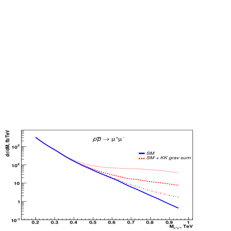
Figure 1: Dilepton invariant mass distribution for parameter $\frac{0.91}{\Lambda_{\pi}^{2}m_{1}^{2}}\times{TeV^{4}}$=0.66 (dashed-dotted line), 1.82 (dashed line), 4 (dotted line) for the Tevatron

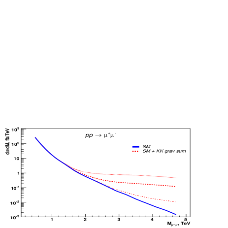
Figure 2: Dilepton invariant mass distribution for parameter $\frac{0.91}{\Lambda_{\pi}^{2}m_{1}^{2}}\times{TeV^{4}}$=0.0014 (dashed-dotted line), 0.0046 (dashed line), 0.01 (dotted line) for the LHC

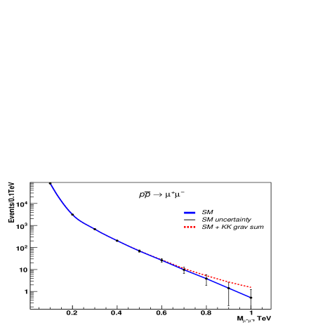
Figure 3: Dilepton invariant mass distribution for $95\%$ CL parameter $\frac{0.91}{\Lambda_{\pi}^{2}m_{1}^{2}}\times{TeV^{4}}$=0.66 for the Tevatron ($L=10{fb}^{-1}$)

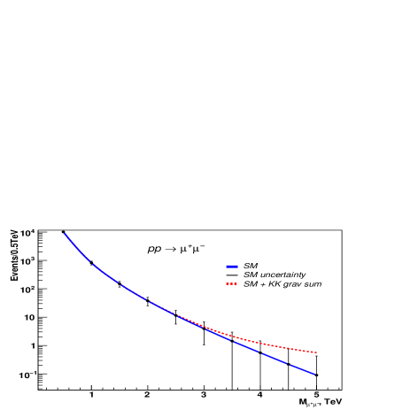
Figure 4: Dilepton invariant mass distribution for $95\%$ CL parameter $\frac{0.91}{\Lambda_{\pi}^{2}m_{1}^{2}}\times{TeV^{4}}$=0.0014 for the LHC ($L=100{fb}^{-1}$)

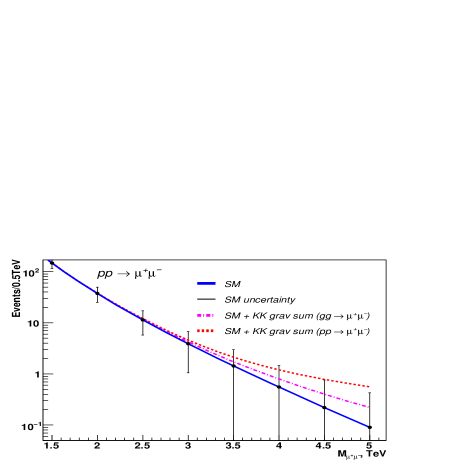
Figure 5: Dilepton invariant mass distribution for $95\%$ CL coupling parameter for the LHC. The dashed-dotted line corresponds to SM + KK sum ($gg\to\mu^{+}\mu^{-}$), the dashed line corresponds to SM + KK sum ($pp\to\mu^{+}\mu^{-}$) process.

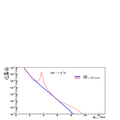
Figure 6: Dilepton invariant mass distribution from the SM (solid line) and from the SM plus sum of KK modes including the first KK resonance with $M_{res}=3.83\leavevmode\nobreak\ TeV$, $\Gamma_{res}=0.08\leavevmode\nobreak\ TeV$, $\Lambda_{\pi}=8\leavevmode\nobreak\ TeV$ (dashed line) for the LHC

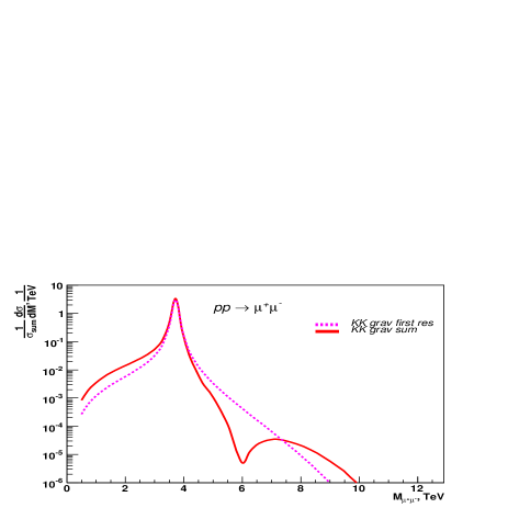
Figure 7: The normalized dilepton invariant mass distribution from the first KK resonance plus the sum of KK tower states starting from the second mode (solid line) and from the first KK resonance only (dashed line) for $M_{res}=3.83\leavevmode\nobreak\ TeV$, $\Gamma_{res}=0.08\leavevmode\nobreak\ TeV$, $\Lambda_{\pi}=8\leavevmode\nobreak\ TeV$ for the LHC

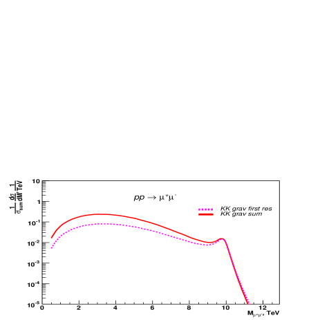
Figure 8: The normalized dilepton invariant mass distribution from the sum of KK tower states starting from the first KK mode (solid line) and from the first KK mode only (dashed line) for $M_{res}=10\leavevmode\nobreak\ TeV$, $\Gamma_{res}=0.5\leavevmode\nobreak\ TeV$, $\Lambda_{\pi}=14\leavevmode\nobreak\ TeV$ for the LHC

One of the effects in searches for KK resonances below the production threshold of the first state is an enhancement of the effective coupling due to KK summation in comparison to the first mode contribution below the threshold only. For the considered case of the stabilized RS model one has a factor

$$\sum_{n\neq 0}\frac{(\psi^{(n)}(L))^{2}}{m_{n}^{2}}\approx 1.82\frac{(\psi^{(1)}(L))^{2}}{m_{1}^{2}}\,.$$

This leads to an increase by $1.82^{2}\approx 3.3$ times in the production rate (for the case of one flat extra dimension this factor is $1.64=>\sum\frac{1}{n^{2}}=\pi^{2}/6$ being numerically close to the warped case).

To illustrate changes in distributions due to KK tower contributions we run simulations for two parameter points with the first KK resonance being in and out of directly detectable regions. The first point ($m_{1}=3.83\leavevmode\nobreak\ TeV$, $\Lambda_{\pi}=8\leavevmode\nobreak\ TeV$, $\Gamma_{1}=0.08\leavevmode\nobreak\ TeV$) was already discussed in Section 3. Such an RS resonance (see Fig. 8) is close to the direct reach limits expected for the LHC [17]. For the second point ($m_{1}=10\leavevmode\nobreak\ TeV$, $\Lambda_{\pi}=14\leavevmode\nobreak\ TeV$, $\Gamma_{1}=0.5\leavevmode\nobreak\ TeV$) the mass of the first KK excitation is close to the collider energy limit, and it is not directly observable. For both points we can use the low-energy effective Lagrangian approach. The effective Lagrangian allows us in both cases to sum up the contributions from all the KK modes or from all except the first one, and in this way to take into account their influence on the background tail. As one can see from Fig. 8 and Fig. 8, the additional substrate from the KK tower increases the production rate more than 3 times in the invariant mass region below the resonance mass. The situation is significantly different above the resonance, where in addition to the resonance pike there is an area with a minimum due to a destructive interference between the first KK resonance and the remaining KK tower contribution. This local minimum takes place at the value of invariant mass $M_{min}\approx 1.5m_{1}$. The growth of the invariant mass after the minimum is strongly suppressed by parton distribution functions leading to an additional bump in the invariant mass shape. But this bump is unlikely to be visible in the experiment on top of the SM background as shown in Fig.8.

In conclusion of this part, one should stress that in order to perform correct searches for KK resonances not only interferences with the SM if nonvanishing and computed NLO QCD corrections [36] should be included into corresponding generators, but also the influence of those KK states, which are not reachable directly.

4 Conclusion

In the present paper we have continued studies of the effects that appear in theories with extra space dimensions due to the exchange of directly unaccessible KK modes of the fields propagating in the bulk when the fundamental energy scale that defines these masses is larger than the typical collision energies $1-10\leavevmode\nobreak\ TeV$. We have derived the effective Lagrangian resulting from the exchange of these KK modes in the stabilized RS model. Such a Lagrangian has a simple structure of a product of two currents, corresponding to the zero mode of a bulk field, multiplied by an effective coupling constant of a dimension depending on the spin of the bulk field. The exact value of this coupling is model dependent and has to be calculated for each model separately. In fact, this structure is reminiscent of the Fermi interaction. Obviously, if the bulk field is the gravity field, then the corresponding current is just the standard energy-momentum tensor of the SM fields (see Appendix A). A delicate nuance in the case of the stabilized RS1 model is that the multidimensional metric has both tensor and scalar massive degrees of freedom, the latter coupled to the trace of the energy-momentum tensor or to its anomaly in the case of massless SM fields. It is shown explicitly that the contributions of the scalar modes are much smaller than those of the tensor modes.

The Feynman rules for the new effective 4-particle interaction vertices of the Standard model fields have been incorporated into the CompHEP computer program, and explicit formulas for the differential and total cross sections for a number of processes, generated by these effective Lagrangians, are presented in Appendix B. For completeness we have included into the symbolic formulas the final state particle masses and contributions of virtual graviton and radion KK modes.

Using these results, we have calculated and plotted the contributions due to the multidimensional gravity to the Drell-Yan production processes for the Tevatron and LHC energies for a number of the stabilized RS model parameter points. It was clearly demonstrated that an enhancement of the effective coupling due to KK summation in comparison to the first mode contribution only leads to an increase of the collider potential to probe the first mode mass below the threshold of its production, the mass being significantly larger than the collision energies. In the case, where the first mode mass is in the accessible energy range, but all the other modes are out of this range, summation of all the modes contributions starting from the second one leads to a significant change of the shape of the Breit-Wigner distribution. The latter case occurs for the considered explicit example in the stabilized Randall-Sundrum model.

We have calculated the effective couplings for this case. To this end, we have used both analytical results and numerical estimates for the wave functions of tensor and scalar modes and performed an approximate summation of the series of inverse mass squared of the KK excitations. For a choice of the parameters of the model, where the effective energy scale $M\sim 1\leavevmode\nobreak\ TeV$ and the other parameters are such that the metric of the stabilized RS model with the radion mass of the order of $2\leavevmode\nobreak\ TeV$ is similar to that of the unstabilized one, we found explicit formula (19) for the effective Lagrangian. For this particular choice of the parameters the first KK graviton and the radion masses are beyond the energy range directly accessible at the Tevatron and within this range at the LHC. However the value of the effective coupling in (19) is too small for deviations from the SM tails to be observed and to probe the masses below the production threshold at the Tevatron energies. For the LHC the first KK and the radion masses are within the directly accessible region. In this case in order to perform correct searches for the tensor resonances and to model the distribution tails one should sum up the contributions from all the other KK modes and take into account their interference with the resonances. It is worth pointing out that this summation of the contributions of the massive tensor modes is also needed for modeling the background in searches for the light radion, whose coupling to the SM fields turns out to be larger, than in the case of the heavy radion.

Acknowledgments

The authors are grateful to Prof. P.F. Ermolov for useful discussions and support. The work was supported by the Russian Ministry of Education and Science under Grant No. NS-1456.2008.2 and by the RFBR Grant Nos. 08-02-91002-CERN_-a and 08-02-92499-CNRSL_-a. M.S. acknowledges support of grant for young scientists under Grant No. MK-5602.2008.2 of the President of Russian Federation. V.B. and M.S. also acknowledge support of grant of the ”Dynasty” Foundation.

5 Appendix A: Energy-momentum tensors for free SM fields

The Lagrangian and the energy-momentum tensor for fermions:

$$L_{\Psi}=\frac{i}{2}\left(\bar{\Psi}\gamma^{\mu}\partial_{\mu}\Psi-\partial_{\mu}\bar{\Psi}\gamma^{\mu}\Psi\right)-m_{\Psi}\bar{\Psi}\Psi$$ (23)

$$T^{\Psi}_{\mu\nu}=\frac{i}{4}\left(\bar{\Psi}\gamma_{\mu}\partial_{\nu}\Psi+\bar{\Psi}\gamma_{\nu}\partial_{\mu}\Psi-\partial_{\nu}\bar{\Psi}\gamma_{\mu}\Psi-\partial_{\mu}\bar{\Psi}\gamma_{\nu}\Psi\right)-$$ (24)

$$-\eta_{\mu\nu}\left(\frac{i}{2}\bar{\Psi}\gamma^{\rho}\partial_{\rho}\Psi-\frac{i}{2}\partial_{\rho}\bar{\Psi}\gamma^{\rho}\Psi-m_{\Psi}\bar{\Psi}\Psi\right)$$

$${T^{\Psi}}^{\mu}_{\mu}=-\frac{3i}{2}\left(\bar{\Psi}\gamma^{\mu}\partial_{\mu}\Psi-\partial_{\mu}\bar{\Psi}\gamma^{\mu}\Psi\right)+4m_{\Psi}\bar{\Psi}\Psi$$ (25)

The Lagrangian and the energy-momentum tensor for massive vector bosons (Z-boson):

$$L_{Z}=-\frac{1}{4}Z_{\mu\nu}Z^{\mu\nu}+\frac{m^{2}_{Z}}{2}Z^{\mu}Z_{\mu}$$ (26)

$$T^{Z}_{\mu\nu}=-Z_{\mu\rho}Z_{\nu\sigma}g^{\rho\sigma}+m^{2}_{Z}Z_{\mu}Z_{\nu}+\eta_{\mu\nu}\left(\frac{1}{4}Z_{\rho\sigma}Z^{\rho\sigma}-\frac{m^{2}_{Z}}{2}Z^{\rho}Z_{\rho}\right)$$ (27)

$${T^{Z}}^{\mu}_{\mu}=-m^{2}_{Z}Z^{\mu}Z_{\mu}$$ (28)

The Lagrangian and the energy-momentum tensor for complex vector bosons (W-bosons):

$$L_{W}=-\frac{1}{2}W^{+}_{\mu\nu}{W^{-}}^{\mu\nu}+m^{2}_{W}W^{+}_{\mu}{W^{-}}^{\mu}$$ (29)

$$T^{W}_{\mu\nu}=-W^{+}_{\mu\rho}W^{-}_{\nu\sigma}g^{\rho\sigma}-W^{+}_{\nu\rho}W^{-}_{\mu\sigma}g^{\rho\sigma}+m^{2}_{W}\left(W^{+}_{\mu}W^{-}_{\nu}+W^{+}_{\nu}W^{-}_{\mu}\right)+$$ (30)

$$+\eta_{\mu\nu}\left(\frac{1}{2}W^{+}_{\rho\sigma}{W^{-}}^{\rho\sigma}-m^{2}_{W}W^{+}_{\rho}{W^{-}}^{\rho}\right)$$

$${T^{W}}^{\mu}_{\mu}=-2m^{2}_{W}W^{+}_{\mu}{W^{-}}^{\mu}$$ (31)

The Lagrangian and the energy-momentum tensor for massless vector bosons (the photon and the gluons):

$$L_{A}=-\frac{1}{4}F_{\mu\nu}F^{\mu\nu}$$ (32)

$$T^{A}_{\mu\nu}=-F_{\mu\rho}F_{\nu\sigma}g^{\rho\sigma}+\eta_{\mu\nu}\frac{1}{4}F_{\rho\sigma}F^{\rho\sigma}$$ (33)

$${T^{A}}^{\mu}_{\mu}=0$$ (34)

The Lagrangian and the energy-momentum tensor for the scalar field (the Higgs field in the unitary gauge):

$$L_{\Phi}=\frac{1}{2}\partial^{\mu}\Phi\partial_{\mu}\Phi-\frac{m^{2}_{\Phi}}{2}\Phi^{2}$$ (35)

$$T^{\Phi}_{\mu\nu}=\partial_{\mu}\Phi\partial_{\nu}\Phi-\eta_{\mu\nu}\left(\frac{1}{2}\partial^{\rho}\Phi\partial_{\rho}\Phi-\frac{m^{2}_{\Phi}}{2}\Phi^{2}\right)$$ (36)

$${T^{\Phi}}^{\mu}_{\mu}=-\partial^{\mu}\Phi\partial_{\mu}\Phi+2m^{2}_{\Phi}\Phi^{2}$$ (37)

6 Appendix B: Partonic total and differential cross sections for $2\to 2$ processes.

Processes $p\bar{p}\to Z^{0}Z^{0}$:

$$\frac{d\hat{\sigma}_{gg\to ZZ}}{dz}=\frac{\kappa^{2}}{16\pi\cdot 16}\beta\left[1+\beta^{2}(z^{2}-1)+\frac{3}{16}\beta^{4}(1-z^{2})^{2}+\right.$$ (38)

$$\left.3\delta^{2}\left(\frac{b(g)}{2g}\right)^{2}\left(1-\frac{2}{3}\beta^{2}+\beta^{4}\right)\right]\hat{s}^{3}$$

$$\hat{\sigma}_{gg\to ZZ}=\frac{\kappa^{2}}{16\pi\cdot 8}\beta\left[1-\frac{2}{3}\beta^{2}+\frac{1}{10}\beta^{4}\leavevmode\nobreak\ \leavevmode\nobreak\ +\leavevmode\nobreak\ \leavevmode\nobreak\ 3\delta^{2}\left(\frac{b(g)}{2g}\right)^{2}\left(1-\frac{2}{3}\beta^{2}+\beta^{4}\right)\right]\hat{s}^{3}$$ (39)

$$\frac{d\hat{\sigma}_{q\bar{q}\to ZZ}}{dz}= \frac{\kappa^{2}}{16\pi\cdot 96}\beta\left[4-2\beta^{2}(z^{2}+1)+3\beta^{4}z^{2}(1-z^{2})\right]\hat{s}^{3}+$$ (40)

$$\frac{\kappa\alpha\cdot c_{1}\beta}{16\cdot 48}\left[\frac{\beta^{2}z^{3}-z}{\xi_{2}}+\beta z(2\beta z+\beta^{2}-3)+\xi_{2}^{2}\beta\cdot\frac{5-\beta^{2}}{\xi_{1}-z}+\frac{\beta^{4}-8\beta^{2}+11}{2}\right]\hat{s}+$$

$$\frac{\pi\cdot\alpha^{2}c_{2}}{16\cdot 48}\left[\frac{2\beta\xi_{1}}{\xi_{1}-z}-\frac{\beta\xi_{2}^{2}}{{(\xi_{1}-z)}^{2}}+\frac{4\xi_{2}}{\xi_{1}^{2}-z^{2}}-\beta\right]\frac{1}{\hat{s}}$$

$$\hat{\sigma}_{q\bar{q}\to ZZ}= \frac{\kappa^{2}}{16\pi\cdot 12}\beta\left[1-\frac{2}{3}\beta^{2}+\frac{1}{10}\beta^{4}\right]\hat{s}^{3}+$$ (41)

$$\frac{\kappa\alpha\cdot c_{1}}{16\cdot 48}\left[(5-\beta^{2})\frac{(1-\beta^{2})^{2}}{2}\ln{\left|\frac{1+\beta}{1-\beta}\right|}+\beta^{5}-\frac{20}{3}\beta^{3}+11\beta\right]\hat{s}+$$

$$\frac{\pi\cdot\alpha^{2}c_{2}}{16\cdot 24}\left[\left(1+\beta^{2}+4\cdot\frac{1-\beta^{2}}{1+\beta^{2}}\right)\ln{\left|\frac{1+\beta}{1-\beta}\right|}-2\beta\right]\frac{1}{\hat{s}}$$

Processes $p\bar{p}\to l^{+}l^{-}$:

$$\frac{d\hat{\sigma}_{gg\to l^{+}l^{-}}}{dz}=\frac{\kappa^{2}}{16\pi\cdot 64}\beta^{3}\left[2(1-z^{2})-\beta^{2}(1-z^{2})^{2}\right]\hat{s}^{3}$$ (42)

$$\hat{\sigma}_{gg\to l^{+}l^{-}}=\frac{\kappa^{2}}{16\pi\cdot 24}\beta^{3}\left[1-\frac{2}{5}\beta^{2}\right]\hat{s}^{3}$$ (43)

$$\frac{d\hat{\sigma}_{q\bar{q}\to l^{+}l^{-}}}{dz}= \frac{\kappa^{2}}{16\pi\cdot 32\cdot 3}\beta^{3}\left[(z^{2}+1)+4\beta^{2}z^{2}(z^{2}-1)\right]\hat{s}^{3}+$$ (44)

$$\frac{\kappa\alpha}{16\cdot 3}\left[z\beta^{2}(1-\beta^{2}+z^{2}\beta^{2})\left(2Q_{q}-2v_{l}v_{q}\chi_{1}\right)+(1-3z^{2})\beta^{3}a_{l}a_{q}\chi_{1}\right]\hat{s}+$$

$$\frac{\alpha^{2}\pi}{2\cdot 3}\left[(2\beta-\beta^{3}+\beta^{3}z^{2})\left(Q_{q}^{2}-2\chi_{1}Q_{q}v_{l}v_{q}+\chi_{2}(a_{l}^{2}+v_{l}^{2})(a_{q}^{2}+v_{q}^{2})\right)+\right.$$

$$\left.2\beta^{2}z(-2\chi_{1}Q_{q}+4\chi_{2}v_{l}v_{q})a_{l}a_{q}+2\chi_{2}(a_{l}^{2}+v_{l}^{2})a_{q}^{2}(\beta^{3}-\beta)\right]\frac{1}{\hat{s}}$$

$$\hat{\sigma}_{q\bar{q}\to l^{+}l^{-}}= \frac{\kappa^{2}}{16\pi\cdot 36}\beta^{3}\left[1-\frac{2}{5}\beta^{2}\right]\hat{s}^{3}+$$ (45)

$$\frac{\alpha^{2}\pi}{3}\left[(2\beta-\beta^{3}+\frac{1}{3}\beta^{3})\left(Q_{q}^{2}-2\chi_{1}Q_{q}v_{l}v_{q}+\chi_{2}(a_{l}^{2}+v_{l}^{2})(a_{q}^{2}+v_{q}^{2})\right)+\right.$$

$$\left.2\chi_{2}(a_{l}^{2}+v_{l}^{2})a_{q}^{2}(\beta^{3}-\beta)\right]\frac{1}{\hat{s}}$$

Processes for linear colliders:

$$\frac{d\hat{\sigma}_{e^{+}e^{-}\to q^{+}q^{-}}}{dz} =9\cdot\frac{d\hat{\sigma}_{q\bar{q}\to e^{+}e^{-}}}{dz}$$ (46)

$$\frac{d\hat{\sigma}_{e^{+}e^{-}\to gg}}{dz}=\frac{\kappa^{2}}{16\pi\cdot 2}(1-z^{4})\hat{s}^{3}$$ (47)

$$\hat{\sigma}_{e^{+}e^{-}\to gg}=\frac{\kappa^{2}}{4\pi\cdot 5}\hat{s}^{3}$$ (48)

$$\frac{d\hat{\sigma}_{\gamma\gamma\to gg}}{dz}=\frac{\kappa^{2}}{16\pi\cdot 2}(1+6z^{2}+z^{4})\hat{s}^{3}$$ (49)

$$\hat{\sigma}_{\gamma\gamma\to gg}=\frac{\kappa^{2}}{\pi\cdot 5}\hat{s}^{3}$$ (50)

Total width for the KK graviton resonance

$$\Gamma^{tot}_{n}= \frac{M_{n}^{3}}{\Lambda_{\pi}^{2}\cdot 4\pi\cdot 5}\left[\frac{9}{4}+\frac{1}{4}\left(\frac{13}{12}+\frac{14}{3}\frac{M_{Z}^{2}}{M_{n}^{2}}+4\frac{M_{Z}^{4}}{M_{n}^{4}}\right)\beta_{Z}+\frac{2}{4}\left(\frac{13}{12}+\frac{14}{3}\frac{M_{W}^{2}}{M_{n}^{2}}+4\frac{M_{W}^{4}}{M_{n}^{4}}\right)\beta_{W}\right.$$ (51)

$$\left.+\frac{21}{8}+\left(\frac{3}{8}-\frac{1}{2}\frac{M_{t}^{2}}{M_{n}^{2}}-4\frac{M_{t}^{4}}{M_{n}^{4}}\right)\beta_{t}\right]\approx\frac{M_{n}^{3}}{\Lambda_{\pi}^{2}\cdot 4\pi}\frac{97}{80}$$

where:

$$\hat{s}=x_{1}x_{2}s,$$

$$\beta_{f}=\sqrt{1-\frac{4M^{2}_{f}}{\hat{s}}},\leavevmode\nobreak\ M_{f}\leavevmode\nobreak\ standing\leavevmode\nobreak\ for\leavevmode\nobreak\ the\leavevmode\nobreak\ mass\leavevmode\nobreak\ of\leavevmode\nobreak\ the\leavevmode\nobreak\ final\leavevmode\nobreak\ state\leavevmode\nobreak\ particle,$$

$$z=\cos\theta,\leavevmode\nobreak\ \theta\leavevmode\nobreak\ denoting\leavevmode\nobreak\ the\leavevmode\nobreak\ partonic\leavevmode\nobreak\ center\leavevmode\nobreak\ of\leavevmode\nobreak\ mass\leavevmode\nobreak\ scattering\leavevmode\nobreak\ angle,$$

$$\theta_{W}\leavevmode\nobreak\ being\leavevmode\nobreak\ the\leavevmode\nobreak\ Weinberg\leavevmode\nobreak\ angle,$$

$$\kappa=\frac{0.91}{\Lambda_{\pi}^{2}m_{1}^{2}},\leavevmode\nobreak\ with\leavevmode\nobreak\ \Lambda_{\pi}\leavevmode\nobreak\ being\leavevmode\nobreak\ a\leavevmode\nobreak\ coupling\leavevmode\nobreak\ constant\leavevmode\nobreak\ of\leavevmode\nobreak\ the\leavevmode\nobreak\ first\leavevmode\nobreak\ KK\leavevmode\nobreak\ resonance\leavevmode\nobreak\ and\leavevmode\nobreak\ its\leavevmode\nobreak\ mass\leavevmode\nobreak\ m_{1},$$

$$a_{l}=-1,$$

$$v_{l}=-1+4\sin^{2}\theta_{W},$$

$$a_{q}=2T_{3q},$$

$$v_{q}=2T_{3q}-4Q_{q}sin^{2}\theta_{W},$$

$$Q_{q}\leavevmode\nobreak\ denoting\leavevmode\nobreak\ the\leavevmode\nobreak\ charge\leavevmode\nobreak\ of\leavevmode\nobreak\ the\leavevmode\nobreak\ quark,$$

$$T_{3q}=\pm\frac{1}{2}\leavevmode\nobreak\ for\leavevmode\nobreak\ up/down-type\leavevmode\nobreak\ quarks,$$

$$\xi_{1}=\frac{1+\beta^{2}}{2\beta},\leavevmode\nobreak\ \leavevmode\nobreak\ \xi_{2}=\frac{1-\beta^{2}}{2\beta},$$

$$c_{1}=\frac{a_{q}^{2}+v_{q}^{2}}{\sin^{2}\theta_{W}\cos^{2}\theta_{W}},\leavevmode\nobreak\ \leavevmode\nobreak\ c_{2}=\frac{6a_{q}^{2}v_{q}^{2}+a_{q}^{4}+v_{q}^{4}}{\sin^{4}\theta_{W}\cos^{4}\theta_{W}}$$

$$\chi_{1}=\frac{1}{16\sin^{2}\theta_{W}\cos^{2}\theta_{W}}\cdot\frac{s(s-M_{Z}^{2})}{(s-M_{Z}^{2})^{2}+M_{Z}^{2}\Gamma_{Z}^{2}},$$

$$\chi_{2}=\frac{1}{256\sin^{4}\theta_{W}\cos^{4}\theta_{W}}\cdot\frac{s^{2}}{(s-M_{Z}^{2})^{2}+M_{Z}^{2}\Gamma_{Z}^{2}}\,.$$

References

- [1] S. Weinberg, Physica A 96 (1979) 327.
- [2] W. Buchmuller and D. Wyler, Nucl. Phys. B 268 (1986) 621.
- [3] C. P. Burgess and D. London, Phys. Rev. D 48 (1993) 4337 [arXiv:hep-ph/9203216].
- [4] C. P. Burgess, S. Godfrey, H. Konig, D. London and I. Maksymyk, Phys. Rev. D 49 (1994) 6115 [arXiv:hep-ph/9312291].
- [5] K. Whisnant, J. M. Yang, B. L. Young and X. Zhang, Phys. Rev. D 56 (1997) 467 [arXiv:hep-ph/9702305].
- [6] J. M. Yang and B. L. Young, Phys. Rev. D 56 (1997) 5907 [arXiv:hep-ph/9703463].
- [7] E. Boos, L. Dudko and T. Ohl, Eur. Phys. J. C 11 (1999) 473 [arXiv:hep-ph/9903215].
- [8] P. M. Ferreira and R. Santos, Phys. Rev. D 74 (2006) 014006 [arXiv:hep-ph/0604144].
- [9] I. Antoniadis, Phys. Lett. B 246 (1990) 377.
- [10] I. Antoniadis and K. Benakli, Phys. Lett. B 326 (1994) 69 [arXiv:hep-th/9310151].
- [11] T. G. Rizzo, arXiv:hep-ph/9910255.
- [12] C. D. Carone, Phys. Rev. D 61 (1999) 015008 [arXiv:hep-ph/9907362].
- [13] H. Davoudiasl, J. L. Hewett and T. G. Rizzo, Phys. Lett. B 473 (2000) 43 [arXiv:hep-ph/9911262].
- [14] T. G. Rizzo, Phys. Rev. D 61 (2000) 055005 [arXiv:hep-ph/9909232].
- [15] T. G. Rizzo and J. D. Wells, Phys. Rev. D 61 (1999) 016007 [arXiv:hep-ph/9906234].
- [16] J. L. Hewett, Phys. Rev. Lett. 82 (1999) 4765.
- [17] H. Davoudiasl, J. L. Hewett and T. G. Rizzo, Phys. Rev. Lett. 84 (2000) 2080 [arXiv:hep-ph/9909255].
- [18] L.D. Landau, E.M. Lifshitz, ”The Classical Theory of Fields”, Pergamon Press, Oxford (1975).
- [19] T. Appelquist, H. C. Cheng and B. A. Dobrescu, Phys. Rev. D 64 (2001) 035002 [arXiv:hep-ph/0012100].
- [20] V. A. Rubakov, Phys. Usp. 44, 871 (2001) [arXiv:hep-ph/0104152].
- [21] N. Arkani-Hamed, S. Dimopoulos and G. R. Dvali, Phys. Lett. B 429 (1998) 263 [arXiv:hep-ph/9803315].
- [22] L. Randall and R. Sundrum, Phys. Rev. Lett. 83, 3370 (1999) [arXiv:hep-ph/9905221].
- [23] O. DeWolfe, D. Z. Freedman, S. S. Gubser and A. Karch, Phys. Rev. D 62 (2000) 046008 [arXiv:hep-th/9909134].
- [24] E. E. Boos, I. P. Volobuev, Y. A. Kubyshin and M. N. Smolyakov, Class. Quant. Grav. 19, 4591 (2002) [arXiv:hep-th/0202009].
- [25] E. E. Boos, Y. S. Mikhailov, M. N. Smolyakov and I. P. Volobuev, Mod. Phys. Lett. A 21 (2006) 1431 [arXiv:hep-th/0511185].
- [26] E. E. Boos, Y. S. Mikhailov, M. N. Smolyakov and I. P. Volobuev, Nucl. Phys. B 717 (2005) 19 [arXiv:hep-th/0412204].
- [27] G. F. Giudice, R. Rattazzi and J. D. Wells, Nucl. Phys. B 595 (2001) 250 [arXiv:hep-ph/0002178].
- [28] C. Csaki, M. L. Graesser and G. D. Kribs, Phys. Rev. D 63 (2001) 065002 [arXiv:hep-th/0008151].
- [29] A. K. Gupta, N. K. Mondal and S. Raychaudhuri, arXiv:hep-ph/9904234.
- [30] K. m. Cheung and G. L. Landsberg, Phys. Rev. D 62, 076003 (2000) [arXiv:hep-ph/9909218].
- [31] E. Boos et al. [CompHEP Collaboration], Nucl. Instrum. Meth. A 534, 250 (2004) [arXiv:hep-ph/0403113].
-
[32]
J. A. M. Vermaseren,
arXiv:math-ph/0010025;
J. A. M. Vermaseren, Nucl. Instrum. Meth. A 559 (2006) 1. - [33] V. M. Abazov et al. [D0 Collaboration], Phys. Rev. Lett. 102, 051601 (2009) [arXiv:0809.2813 [hep-ex]].
- [34] G. L. Bayatian et al. [CMS Collaboration], J. Phys. G 34 (2007) 995.
- [35] G. F. Giudice, R. Rattazzi and J. D. Wells, Nucl. Phys. B 544, 3 (1999) [arXiv:hep-ph/9811291].
-
[36]
P. Mathews, V. Ravindran, K. Sridhar and W. L. van Neerven, Nucl. Phys. B 713 (2005) 333 [arXiv:hep-ph/0411018];
P. Mathews, V. Ravindran and K. Sridhar, JHEP 0510 (2005) 031 [arXiv:hep-ph/0506158];
P. Mathews and V. Ravindran, Nucl. Phys. B 753 (2006) 1 [arXiv:hep-ph/0507250];