Latitudinal variation of the solar photospheric intensity

Abstract

We have examined images from the Precision Solar Photometric Telescope (PSPT) at the Mauna Loa Solar Observatory (MLSO) in search of latitudinal variation in the solar photospheric intensity. Along with the expected brightening of the solar activity belts, we have found a weak enhancement of the mean continuum intensity at polar latitudes (continuum intensity enhancement $\sim 0.1-0.2\%$ corresponding to a brightness temperature enhancement of $\sim 2.5{\rm K}$). This appears to be thermal in origin and not due to a polar accumulation of weak magnetic elements, with both the continuum and CaIIK intensity distributions shifted towards higher values with little change in shape from their mid-latitude distributions. Since the enhancement is of low spatial frequency and of very small amplitude it is difficult to separate from systematic instrumental and processing errors. We provide a thorough discussion of these and conclude that the measurement captures real solar latitudinal intensity variations.

1 Introduction

Latitudinal variations in the thermal structure of the solar convective envelope have been implied or required by theories ranging from non-general-relativistic gravity (Dicke, 1964) to those explaining the solar differential rotation (e.g. Kitchatinov & Rüdiger, 1995; Durney, 1999; Rempel, 2005; Miesch et al., 2006), meridional circulation, and torsional oscillations (Spruit, 2003). Models of the solar differential rotation and meridional circulation reproduce the observed helioseismic rotation profiles (Thompson et al., 1996; Schou et al., 1998) best when baroclinicity is introduced via a latitudinal temperature gradient in region of the solar tachocline which spreads into the convection zone proper by turbulent convection (Rempel, 2005; Miesch et al., 2006). While it is estimated from such models that in the solar photosphere the pole may be as much as a few degrees warmer and the mid-latitudes a couple of degrees cooler than the equatorial region (e.g Brun & Toomre, 2002; Miesch et al., 2006), these estimates are model dependent and measurements have proven difficult. The difficulties arise because of the intrinsically low amplitude thermal signal expected and the presence of magnetic structures which introduce small scale intensity fluctuations of comparable or greater amplitude. Thus, previous observations have yielded wide ranging results (Table 1).

Here we examine full disk images from the Precision Solar Photometric Telescope (PSPT) at the Mauna Loa Solar Observatory (MLSO). The telescope should by design readily allow measurement of latitudinal temperature variations if they are a few degrees in magnitude. In §2 below we review the telescope capabilities and data processing techniques necessary to realize those. In §3 we present the results obtained and in §4 discuss the uncertainties in these due to random and systematic errors. Finally, we conclude in §5 by putting our methods and results in the context of previous measurements.

2 The PSPT data

The PSPT at the MLSO is a small (15 cm) refracting telescope designed for photometric solar observations with the aim of achieving an unprecedented 0.1% pixel-to-pixel relative photometric precision. It acquires full-disk solar images on a $2048\times 2048$ CCD array ($\sim 1\arcsec$/pixel) in three wavelength bands: blue continuum ($409.412$ FWHM $0.267$nm), red continuum ($607.095$ FWHM $0.458$), and CaIIK ($393.415$ FWHM $0.273$nm). The red continuum band is quite clear of absorption lines while the blue continuum is not (profiles superimposed on reference spectra are available on the PSPT web site). The quiet-Sun formation heights (relative to optical depth unity at 500 nm and over the FWHM of the filter band) for these wavelengths are approximately (Rast et al., 2001): blue continuum, -10 to 35 km; red continuum, 0 to 50 km; and CaIIK line, 900 to 1660 km (line core) and 0 to 260 km (line wings). The PSPT concept and prototype are described in more detail in Coulter & Kuhn (1994).

2.1 Gain correction

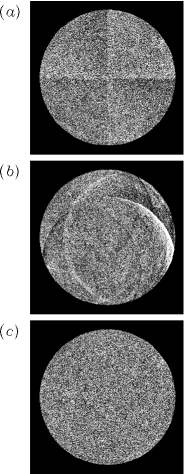
Figure 1: Examples of failed ($a$ and $b$) and successful ($c$) gain correction attempts, illustrated with histogram-equalized contrast images. Note that the failed attempts chosen for this illustration have especially large and obvious problems which can be seen even in unequalized high contrast images. This is not usually the case, and most image defects remaining after ‘flat-fielding’ are of much lower amplitude and can only be faintly seen after histogram equalization of the image. No MLSO PSPT data is considered acceptable if the amplifier induced quadrant structure is at all apparent in histogram equalized images. Every attempt is made to arrive at a contrast image showing no residual arc structure introduced by the Kuhn et al. (1991) algorithm.

The PSPT camera readout occurs in quadrants through four amplifiers of differing gain. In order to achieve in data images the photometric precision promised by the instrument design, these and other spatial variations in the detector must be determined to an equivalent accuracy. We accomplish this using a version of the algorithm of Kuhn et al. (1991) applied to sixteen offset images of the Sun recorded once per day. By assuming that the Sun is unchanged between each of these offset images and comparing both pixel intensities at identical image locations and pixel gains at identical detector locations, the procedure captures a best fit spatial mapping to the differences between the offset image intensities which when corrected would minimize their differences. The procedure is sensitive to a variety of contributions, including, those fixed on the detector plane (such as pixel to pixel gain variation or the amplifier induced quadrants), those resulting from variation in the offset image light path (such as filter density variations), those resulting from image evolution during the acquisition sequence (seeing variations), and any others which are not stationary with respect to the solar image. The sensitivity to variation in atmospheric seeing during the course of the sequence is particularly troublesome, and a usable ‘flat-field’ is not obtained daily. Figures 1$a$ and $b$ display, with histogram equalization of the intensity (e.g. Russ, 1999), contrast images (see below) which are produced from the raw data using particularly poor flat-fields. The gain correction in ($a$) failed to remove the amplifier induced quadrants and in ($b$) introduced arc shaped defects related to the offset image positions in the flat-field algorithm. Such flat-fields would never be used in the image processing (Figure 1$c$ displays the image as actually processed for this study). All PSPT images from the MLSO are inspected individually using histogram equalization of the contrast intensity and, if necessary, reprocessed with a flat-field from a neighboring date until a gain correction is made which leaves no visible quadrant structure and no or few algorithm related defects in the image. This kind of inspection is capable of identifying defects remaining in individual images to very low amplitudes (below 0.1%), but, since the flat-field image offset positions are a fixed sequence on the detector, defects remaining in the images below human visual acuity are the largest known source of systematic error in the data. We discuss these in detail in §4.

2.2 Center-to-limb variation

While the solar center-to-limb intensity variation and its possible temporal variability has intrinsic importance, reflecting the mean thermodynamic structure of the outer layers of the star, here we are interested in spatial variations (in particular latitudinal variation) about this underlying azimuthally invariant limb-darkening profile, and so must also measure it with precision. We employ a procedure which identifies quiet sun pixels in the image and performs a simultaneous least-squares fit to the intensity of these to determine the coefficients of a truncated series of Legendre polynomials in radius $P_{m}(r)$ and Fourier modes in central angle:

$$I_{0}(r,\theta)=\sum_{n}\sum_{m}\left[A_{nm}P_{m}(r)\cos(n\theta)+B_{nm}P_{m}(r)\sin(n\theta)\right]$$

truncated to $m\leq 6$ and $n\leq 2$, where $r$ and $\theta$ are polar coordinates with the origin at the solar disk center. Quiet sun pixels are taken as those within $\pm 2.5\sigma$, in red and blue continuum, or $-2.5<\sigma<0.0$, in CaIIK images, of the median intensity in about seventy-five equal area annuli centered around the solar disk center (the annulus area is fixed so the number employed is slightly dependent on filter band and time of year). The orthogonality of the fitted functions allows capture, with little mixing, of both the solar center-to-limb variation and any residual dipolar (linear gradient) or quadrupolar (quadrant structure) artifacts present in the image. We note that, because the Fourier phase at a given radius is independent from that at another, this formalism allows for the removal of a warped gradient or quadrant surface (the Fourier fit can rotate with azimuth at a given $r$). This is a powerful tool in removing large scale image defects (see §4). We also note that the use of the contrast images $I_{c}=(I-I_{0})/I_{0}$, where $I$ is the intensity measured at each pixel and $I_{0}$ is the fit to the solar center-to-limb variation and residual defects, in this study implies that the intensity measurements reported here are relative to a particular center-to-limb profile removed. That profile was calculated for a particular subset of quiet Sun pixels in each image (defined above), and other pixel subsets in the resulting contrast image will show center-to-limb brightening or darkening depending on their activity level in relation to those used to compute the center-to-limb function removed.

2.3 Data selection and alignment

We have selected fifty six of the best contrast image triplets from the MLSO PSPT image archive, spanning the period from March 2005 to July 2006. The complete list of selected image triplets is given in Table 2. Image quality was determined using two criterion: quality of the gain correction (§2.1) and atmospheric seeing conditions. Seeing was estimated based on a measure of the red continuum solar limb width as determined from a Gaussian profile fit to intensity values limb-ward of the inflection point in the four grid aligned directions from the solar disk center. Only images with an average red continuum Gaussian FWHM of less than 2.5 pixels (limb width of 1.25 pixels) were used in this study.

Following selection, each image was resized, rotated, and aligned to a common reference grid in which the solar P0 and B0 angles are zero, i.e., the vertical image axes were aligned with the solar North-South. While these operations require interpolation (bilinear used) and thus introduce error, we have minimized the total impact by combining the procedures into a single interpolative step in heliographic coordinates.

2.4 Activity masks

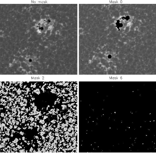
Figure 2: Example applications of CaIIK masks to the same sub-image. Intensity thresholds are used to mask out activity. While Mask 2 eliminates most plage and network elements retaining about 50% of the pixels, Mask 6 retains only 0.15% of the pixels masking out all but the darkest cell centers.

Once aligned, the images can be used to construct averages and masks. Pixel selection by masking (here we define masking as excluding from analysis) is based on using CaIIK intensity as a surrogate for the magnetic flux density (e.g. Skumanich et al., 1975; Schrijver et al., 1989; Harvey & White, 1999; Rast, 2003; Ortiz & Rast, 2005). After sunspots and pores are masked out by thresholding the red continuum contrast intensity (keeping $I_{R}>-0.05$), small magnetic elements show a strong positive correlation between CaIIK intensity and magnetic flux density, even down to very low intensity values (Rast, 2003). Here we apply increasingly severe masks to the images, retaining only pixels in the analysis whose CaIIK intensity falls below the mask value. Table 3 indicates the mask intensity values used in this study, the approximate corresponding magnetic flux density (from Rast, 2003; Ortiz & Rast, 2005), and the average (over the image set) percentage of pixels retained by each. Masks range from very unrestrictive (M0 retains all magnetic activity except sunspots and pores) to very restrictive (application of mask M6 or M7 yields images which retain only the very darkest CaIIK network cell centers). Figure 2 illustrates the effect of applying masks M0, M2, and M6 to a subregion of a typical CaIIK image.

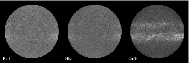
Figure 3: Average contrast image after application of mask M0 to the images at each of the three wavelengths. Magnetic activity in the active belts shows hemispherical asymmetry during the declining phase of Cycle 23. Also faintly visible is the polar brightening which is the subject of this paper. Note that the polar brightening measured is not that due to the extreme limb points, which are somewhat unreliable due to reduced image contributions as a result of the B0 correction. The bulk of the analysis presented in this paper uses pixels from annuli well inside the limb (see Figure 7$a$).

We applied the eight masks based on CaIIK contrast values to the 56 contrast images at all wavelengths and averaged the unmasked pixels to produce mean contrast images at each wavelength and activity level. Examples are shown in Figure 3, where the average image (after mask M0 application) at each wavelength is displayed. The average activity over the nearly 17 months of observation is apparent as bright latitudinal bands across the CaIIK image disk and as limb-brightened faculae in the continuum observations. As has been previously reported for the declining phase of Cycle 23 (Knaack et al., 2004; Zaatri et al., 2006), hemispherical asymmetry in magnetic activity is clearly evident in these average images (it is also seen in a more uniform sampling of the observation period). The continuum images also show a hint of the polar brightening which is the subject of this paper.

In next section we present results obtained largely from the application of masks M0 and M2 which separate plage/network from non-network contributions. Mask M0 removes only sunspots and pores from the images while M2 masks out most network elements (Figure 2). Preliminary results using the more severe mask M6 to remove all but the contributions from the darkest cell centers (these perhaps representative of purely thermal emission from the non-magnetized photosphere) are also presented.

3 Results

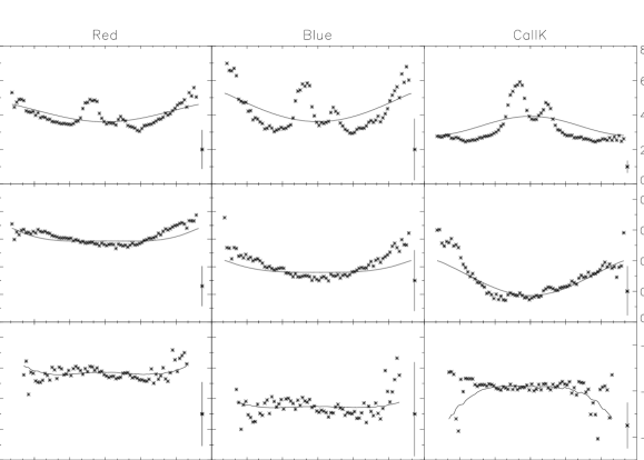
Figure 4: Intensity contrast as a function of latitude for the red, blue and CaIIK wavelengths after application of activity masks, M0, M2 and M6. The vertical scale on the left is common for both the red and blue plots. That for CaIIK is indicated on the right. Solid curves plot the same longitudinal average of the center-to-limb variation as a function of latitude. Vertical bars indicate the largest error estimated from the rms fluctuations in each latitudinal bin.

Using the techniques described we have examined the latitudinal variation of the continuum photospheric intensity in PSPT images. For each activity mask and wavelength, we have longitudinally averaged the mean contrast image over $2\arcdeg$ wide latitudinal bins. The results are shown in Figure 4. To be meaningfully interpreted, the variation with latitude must be compared with the longitudinally averaged center-to-limb variation (CLV) of the mean contrast image (as discussed in §2.1 the unmasked pixels show a CLV relative to that already removed in making the contrast image). This is plotted in Figure 4 with solid curves. If no systematic latitudinal variation in mean intensity existed on the Sun then the measured longitudinally averaged mean contrast would be the same as the longitudinally averaged CLV. This is not the case. Significant (see §4 for discussion of noise properties) variation in the longitudinally averaged intensity is observed with latitude.

Images weakly masked by M0 to remove only sunspot and pore contributions (top row of Figure 4) clearly show enhanced intensity at active region latitudes, as was already apparent in the full disk images of Figure 3. The peak contrast intensities occur near $\pm 12\arcdeg$ latitiude at all wavelengths, with greater enhancement in the southern hemisphere than the northern. Additionally, the images masked by either the M0 or the M2 mask (middle row of Figure 4) show evidence of polar brightening. Mask M2 eliminates most magnetic activity over the solar disk (only pixels whose CaIIK intensities correspond to magnetic flux densities of less than a couple gauss have been kept), and after application of this mask the images show an average $\sim 0.1\%$ enhancement in contrast in the polar region in both the red and blue continuum bands, slightly larger in the blue. The CaIIK contrast for this mask value shows no polar enhancement in the southern hemisphere but some in the northern. This is not yet understood.

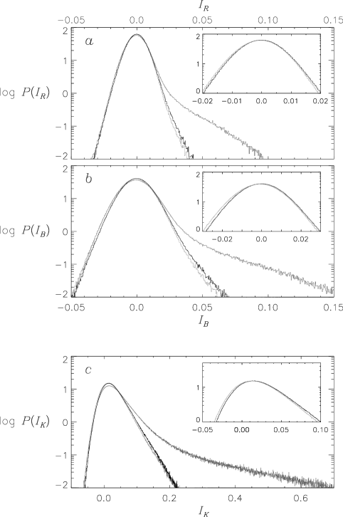
Figure 5: Contrast distributions computed for each of the unmasked images, normalized so that integrated probability is unity and averaged over the 56 individual images in each wavelength. The distributions are those of pixels from an annulus between $\mu=0.3$ and $\mu=0.45$ and separated into polar contributions (black curves), equatorial contributions (dark grey curves), and mid-latitude contributions (light grey curves) as defined in Figure 6. Insets show close-ups of the mid-latitude and polar distribution peaks.

The observed polar continuum enhancement is likely not due to the presence of polar faculae. While these may contribute to the unmasked profiles of M0, they are eliminated by M2 mask as their CaIIK intensity likely exceeds the $I_{K,max}$ threshold. This assertion is supported by the pixel intensity distributions (Figure 5) which show that the polar and mid-latitude distributions have nearly identical shapes, lacking the bright tail of the equatorial distributions. The polar distributions at all wavelengths are shifted as a whole to higher intensity values than their mid-latitude counterparts. This is in agreement with flux measurements using the solar distortion telescope (Kuhn et al., 1988). The lack of any bright CaIIK distribution tail, combined with the shift toward higher intensity in the continuum bands, suggests a thermal non-magnetic origin for the polar brightening. That the CaIIK distribution is also shifted likely results from the fact that PSPT CaIIK filter is sufficiently broad to include a significant photospheric contribution.

Images masked by the even more severe M6 mask exclude all contributions but those from the quietest CaIIK cell centers. Application of this mask is ideal for determination of the latitudinal variation in the thermal structure of the solar photosphere, as virtually all magnetic contributions should be negligible. Unfortunately, the small number of remaining pixels makes this measure subject to large statistical uncertainty. The noise is largely of solar origin (unresolved granulation) and could be addressed with more data. This may be worthwhile, as the preliminary results presented here (bottom row Figure 4) suggest a hint of the expected (Brun & Toomre, 2002; Rempel, 2005; Miesch et al., 2006) increase in photospheric continuum intensity in both the polar and equatorial regions as compared to the solar mid-latitudes. If these increases are found to be significant after analysis of additional data, they would confirm a non-facular origin of the equatorial brightening (Kuhn et al., 1987, 1988), as all facular contributions have likely been eliminated by the severity of the M6 masking.

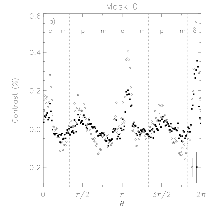
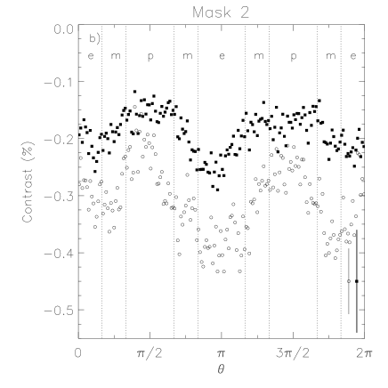
Figure 6: Red (filled squares) and blue (open circles) contrasts in the average M0 and M2 masked images as functions of polar angle $\theta$ around the annulus $0.3<\mu<0.45$. Three sectors in $\theta$, equator, mid-latitudes, and poles, are marked by the letters e, m, and p. Vertical bars indicate the amplitude of the maximum rms fluctuations in any bin.

An alternative way of plotting the latitudinal intensity variations (to further distinguish them from those of the CLV, and later in §4 from systematic error) is to plot the contrast as a function of polar angle $\theta$ on the disk at fixed cosine of the heliocentric angle $\mu$. Since the sampling now occurs at fixed $\mu$, the CLV contributes a constant offset to the measurement (independent of $\theta$). Figures 6$a$ and $b$ present the continuum red and blue contrast intensities in this way after applying masks M0 and M2, respectively. The average contrast values in a ring between $0.3<\mu<0.45$ and for $2\arcdeg$ bins in $\theta$ are plotted, scanning the solar limb counter-clockwise from the west (right hand side of the image). In these plots the equator lies at $\theta=0$, $\pi$ and $2\pi$, while the poles lie at $\pi/2$ and $3\pi/2$. The hemispherically asymmetric north and south activity belts are again apparent in Figure 6$a$ as increases in the red and blue continuum intensities either side of the equator. The polar enhancement is also prominent as are the darker mid-latitudes. Figure 6$b$ further confirms the polar enhancement. After application of mask M2 the polar intensity is about 0.15% larger than that at the equator in the red continuum ($\sim 0.2$% greater at the pole than equator in the blue continuum).

4 Random and Systematic Errors

Random fluctuations in the PSPT images are largely granular in origin and thus of high spatial frequency, follow a $\sqrt{n}$ reduction in amplitude upon image averaging (when the images are separated by more than one granule lifetime), and are well represented by the error bars shown in Figures 4 and 6. Those error bars indicate the maximum rms fluctuations about the latitudinal or $\theta$ bin averages for any of the data points plotted. The variations with latitude or $\theta$ measured are thus significant with respect to small scale random noise. Moreover, smaller subsets of the data images show the same underlying signal, albeit with larger amplitude fluctuations.

The known systematic errors in the data behave differently. They are of large spatial scale and persistent with averaging, and thus pose the greatest challenge to the measurement. The dominant source of known systematic error is the presence of very low amplitude residual image defects which reflect the offset positions used in the  Kuhn et al. (1991) flat-field algorithm (§2.1). Since their location is nearly fixed (somewhat smeared by the P0 and B0 correction during image alignment), they add upon averaging and are faintly visible in the continuum contrast images in Figure 4. This section addresses and quantifies the level of uncertainty introduced by this source of error.

As discussed in § 2.1 the PSPT images are subject to two consecutive image processing stages, the first aimed at removing detector gain variations and the second, combined with the center-to-limb calculation, intended to remove residual dipolar and quadrupolar defects. This second step is necessary, not only to capture the faint defects described above, but also because the flat-field algorithm itself is subject to an intrinsic gradient ambiguity (Kuhn et al., 1991) and can thus introduce or fail to remove linear gradients in the image. The gradient is measured via the $n=1$ Fourier component of the CLV routine. We will see below that the $n=2$ mode proves useful in the further removal of the systematic defects.

In order to assess the efficacy of these techniques, it is useful to apply them to those portions of the image which lie off of the solar limb in the same way as they are applied to the solar disk itself. This allows comparison between the systematic noise contributions to the image and the measured signal, since the signal should be absent off of the solar disk. While the standard PSPT processing procedures correct for the detector gain variation across the entire field of view, they apply the Legendre/Fourier center-to-limb/defect correction only on the solar disk. In this section we thus employ a conceptually (but not mathematically) equivalent procedure which can be readily extended off of the solar limb.

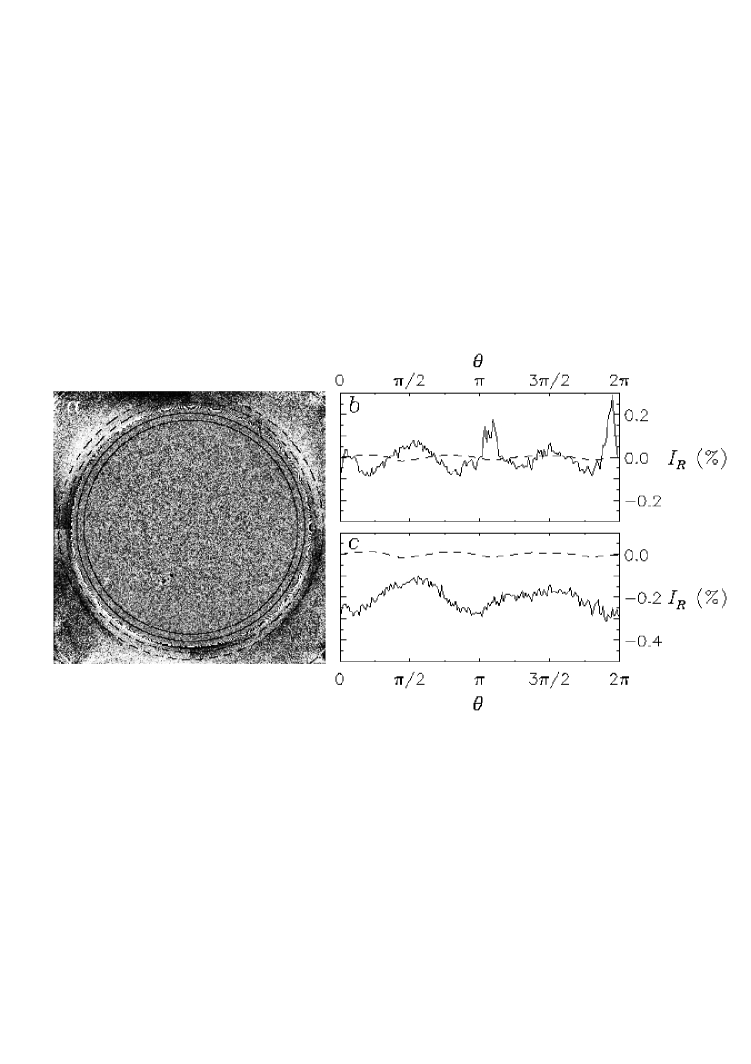
Figure 7: In ($a$), a histogram equalized red contrast image from 14 August 2005 with the CLV and residual defect processing applied to the full field of view (see text). In ($b$) and $c$), average (over all images and in $2\arcdeg$ bins in $\theta$ for the $0.3<\mu<0.45$ annulus) contrast as a function of $\theta$ in two annuli (shown in ($a$)), one off of (dashed curve) and one on (solid curve) the solar disk, after application of masks M0 (in $b$) and M2 (in $c$).

After masking sunspot pixels, we divide the image by the median value of the intensity in very narrow annuli (1000 equal width annuli employed) centered on the solar disk center. This very effectively removes the azimuthally invariant center-to-limb variation on the disk, while performing an equivalent correction off of it. Fourier amplitudes are then calculated, fitting the pixels within each annulus independently with the $n=0-2$ expansion. The dipolar and quadrupolar defect correction is thus extended off of the solar disk. Figure 7$a$ displays a single red continuum image processed in this way after histogram equalization of the contrast intensity. While the large scale defects contributing to systematic error in the analysis are barely visible on the solar disk, where real physical intensity fluctuations dominate the image and the error contrast is low, they are quite apparent as both residual quadrants and flat-field induced arc defects off the limb, where their relative contrast is high due to the low mean intensity values. Figures 7$b$ and $c$ display the mean contrast, after application of masks M0 and M2 respectively, in two annuli (on the disk solid curve, off the disk dashed curve) as a function of $\theta$. These curves are the averages of those obtained from the individual images after shifting appropriately for the solar P0 angle, and the off disk contrast has been scaled down by the ratio of the median intensity in the two annuli. The solid curves are equivalent to the red continuum plots shown in Figures 6$a$ and $b$ but without the B0 correction, and we note the very close similarity to those despite this difference and that of the underlying CLV correction method. What Figure 7 displays in addition to Figures 6 is a measure of the systematic processing errors off of the solar disk (dashed curves). These are much smaller in magnitude than the measured signal on the disk suggesting that the measurement is not dominated by noise.

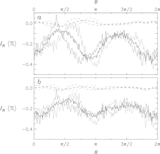
Figure 8: Average (over all images and in $2\arcdeg$ bins in $\theta$ for the $0.3<\mu<0.45$ annulus) contrast as a function of $\theta$ in two annuli, one off of (dashed black curve) and one on (solid black curve) the solar disk (see Figures 7$a$), after application of mask M2. In ($a$) only the $n=0-1$ Fourier modes have been included in the defect correction, in ($b$) $n=0,2$ modes are included. Dark and light grey curves plot the same quantities for images with P0$\ >10$ and P0$\ <-10$ respectively.

Since the measured polar brightening takes a $\cos(2\theta)$ form, it is important to ask if the Fourier mode correction for image defects in fact spuriously introduces the ‘signal’ being measured. Figures 8$a$ and $b$ plot the average contrast (after mask M2 application) as a function of theta after employing only the $n=0-1$ and $n=0-2$ corrections respectively. The amplitude of the polar brightening is reduced, not enhanced by the $2\theta$ correction. It is also apparent that the $2\theta$ correction further reduces the systematic noise off of the solar disk (dashed curves). Moreover, Figures 8$a$ and $b$ plot separately the contributions, both on and off of the disk, made by images with P0$\ >10.0$ and P0$\ <-10.0$ (dark and light grey curves respectively). This is a robust measure of the error contributions to the signal since any real solar measurement should be stationary with respect to this distinction. Without the $2\theta$ correction (Figure 8$a$) the positive and negative P0 curves, from the data both on and off of the disk, are consistently shifted with respect to one another. After application of the $2\theta$ correction (Figure 8$b$) the signals off of the solar disk remains consistently shifted, but those from on the solar disk do not. After the correction, the southern hemisphere signals for positive and negative P0 values show no or even slightly the wrong sense of shift with respect to one another, indicating that they are a property of the solar image and not a defect fixed in the detector plane. The signal in the northern hemisphere still appears to have some noise contribution, but at a much reduced amplitude. This is consistent with our experience with the images, which tend to show more defects in the northern hemisphere in response to the fixed flat-field sequence. We note that this test was also performed on subsets of the data, after selection of just the very best images, and while the random noise levels were higher, the polar brightening always stood out from the systematic error. Moreover, annuli of smaller radius showed the same signal, albeit of decreasing amplitude as expected. We conclude that the Fourier/Legendre CLV processing allows measurement of solar polar brightening at the very limits of the PSPT capabilities.

5 Conclusion

We have measured an enhancement of the photospheric continuum intensity in the solar polar regions using PSPT images. We have carefully examined the properties of the signal and believe it to be of solar origin. Moreover, the properties of the intensity distributions suggest that the signal is thermal not magnetic in origin, although contributions from very weak network elements associated with the pole-ward extending branch of the solar cycle (e.g. Howard & Labonte, 1981; Muller & Roudier, 1984; Sheeley & Warren, 2006) cannot be ruled out without processing significantly more data and employing masking of greater severity. This is planned, but limitations of the current ground based solar photometric observations may make a decisive measurement difficult. Space based imaging photometry would be ideal for this and other intriguing problems. This is particularly true if solar cycle dependencies are to be uncovered.

Such measurements would help constrain global solar models by adding a thermodynamic constraint to the dynamical constraints currently provided by helioseismology (Kuhn et al., 1988). Current numerical simulations seem to show little indication of a local temperature minimum at the equator, as our surface measurement implies, but rather display a mid-latitude minimum with a weak local maximum at the equator and stronger one at the pole. This is true even when a monotonically decreasing pole to equator profile is imposed in the solar tachocline (Rempel, 2005; Miesch et al., 2006). While we find some hint of equatorial brightening after application of our most restrictive activity masks (bottom row Figure 4), it has extremely low amplitude and the measurement is extremely uncertain.

Our efforts can be distinquished from previous work in several ways. Early work (references $1-7$ in Table 1) struggled with instrumental precision, systematic error, and detector gain correction. We too have taken pains to address these. More importantly, no distinction was made in that early work between magnetic and thermal contributions to the signal, other than perhaps qualitative selection of nonactive regions. We have emphasized this distinction by applying a series of masks based on CaIIK intensity to the images before analysis. Previous efforts by Kuhn et al. (references $8-10$ in Table $10$) have, for the most part, also attempted to separate quiet Sun and facular contributions to the latitudinal signal. The approach in those studies differed from ours in that the facular contribution to the latitudinal variation was estimated statistically based on models of the quiet Sun and facular color and intensity distributions. Interestingly, the pole/mid-latitiude temperature contrast measured in those studies is in good agreement with our measurement. The previous authors, however, reported an additional low latitude brightness enhancement, only seeen very marginally, if at all, in our study at the most severe masking levels. We note, that the one measurement of solar latitudinal intensity variation available using spacecraft data (Kuhn et al., 1998) did not remove the facular contribution during analysis. The latitudinal temperature profile obtained in that work looks very similar to our Figure $6a$, also unmasked.

Finally, we caution that our analysis does not completely eliminate possible contributions to the solar photospheric intensity from an abundance of unresolved magnetic elements of very low magnetic flux density. Correlations between magnetic flux density and CaIIK intensity extend to very low values, making masking based on these images possible, but also suggesting continued contamination of the continuum measurements at very low contrasts (Rast 2003). Unambiguous measurement of a strictly thermal signal in the solar photosphere may require space-based full-disk photometric imaging at high precision and resolution over many wavelengths, combined with detailed modeling of the radiation field. Even that effort may be stymied if in fact there is no quiet Sun.

Table 1: Some past observations of latitudinal variation in the solar photospheric temperature

Reference	$T_{pole}-T_{equator}$	Method	Active regions or quiet Sun
	(K)
1	$<3$	limb flux measurements	no distinction
2	0 (within errors)	equivalent width of Fraunhofer lines at limb	no distinction
3	1.5 $\pm$ 0.6	spectrograph scans of CLV	plage region excluded
4	3 $\pm$ 3	Mg I spectra at 50 disk positions	quiet Sun
5	0 $\pm$ 0.6%	equivalent width of Fraunhofer lines at limb	avoid active regions
6	$<1$	IR opacity minimum, grating monochrometer CLV scans	no distinction
7	19 (South pole)	continuum (501.15nm) CLV scans	quiet Sun
7	-19 (North pole)	continuum (501.15nm) CLV scans	quiet Sun
8	1.2 $\pm$ 0.2	limb flux measurements	faculae rejection
9	1.5	limb flux measurements	faculae rejection
10	1.5	MDI images, limb shape and brightness	no distinction

Note. — References: (1) Dicke & Goldenberg (1967); (2) Caccin et al. (1970); (3) Altrock & Canfield (1972b); (4) Rutten (1973); (5) Falciani et al. (1974); (6) Koutchmy et al. (1977); (7) Wittmann (1978); (8) Kuhn et al. (1985, 1987); (9) Kuhn et al. (1988); (10) Kuhn et al. (1998)

Table 2: Census of the observed triplets

Date	Hour	Date	Hour
	(UT)		(UT)
07 Mar 2005	18:50	19 Oct 2005	17:50
17 Mar 2005	17:20	25 Oct 2005	18:30
23 Mar 2005	17:50	25 Oct 2005	18:50
12 Apr 2005	17:40	15 Nov 2005	18:30
13 Apr 2005	17:12	18 Nov 2005	18:02
14 Apr 2005	17:12	19 Nov 2005	18:02
21 Apr 2005	18:20	30 Nov 2005	18:12
25 Jun 2005	17:12	30 Dec 2005	18:12
27 Jun 2005	16:50	31 Dec 2005	18:12
27 Jun 2005	17:50	05 Jan 2006	18:20
06 Jul 2005	17:02	18 Jan 2006	18:30
20 Jul 2005	18:50	02 Feb 2006	19:02
11 Aug 2005	17:02	06 Feb 2006	18:20
14 Aug 2005	17:12	06 Feb 2006	19:02
16 Aug 2005	17:02	08 Feb 2006	18:20
17 Aug 2005	17:30	09 Feb 2006	18:50
21 Aug 2005	17:30	28 Mar 2006	19:12
22 Aug 2005	17:12	07 Apr 2006	18:12
23 Aug 2005	17:30	14 Apr 2006	18:30
23 Aug 2005	17:50	29 Apr 2006	17:12
24 Aug 2005	17:12	03 May 2006	17:12
07 Sep 2005	17:12	04 May 2006	16:50
17 Sep 2005	17:20	04 May 2006	17:12
23 Sep 2005	17:40	18 May 2006	17:20
06 Oct 2005	18:12	18 Jun 2006	18:12
06 Oct 2005	18:30	20 Jun 2006	17:12
14 Oct 2005	18:02	20 Jun 2006	17:50
18 Oct 2005	18:12	14 Jul 2006	17:02

Note. — Observation times indicated are approximate. Each image is an average of 30 exposures aimed at minimizing brightness variations due to solar oscillations. The three filter observations are interleaved (three sequences of 5 blue, 5 CaIIK, 5 red, 5 red, 5 CaIIK, and 5 blue are taken over the course of about 5 minutes) so that the resulting images at each of the three wavelengths may be considered ‘simultaneous’. The imaging begins about three minutes (during which time dark calibrations are made) after the observation time quoted above and used in the image filenames. Actual start and end times of the image sequence can be found in the image headers.

Table 3: Definition of the CaIIK masks

Mask	$I_{R,{\rm min}}$	$I_{K,{\rm max}}$	$B_{\rm max}$	Pixels retained
			(G)	(%)
M0	-0.05	$\cdots$	$\cdots$	99.90
M1	-0.05	0.150	29.0	97.00
M2	-0.05	0.025	2.5	50.00
M3	-0.05	-0.010	0.8	10.00
M4	-0.05	-0.020	0.7	5.00
M5	-0.05	-0.030	0.6	2.00
M6	-0.05	-0.050	0.45	0.15
M7	-0.05	-0.060	0.4	0.04

Note. — Column (1): Mask. (2): Minimum red intensity contrast threshold. (3): Maximum CaIIK intensity contrast threshold. (4): Corresponding magnetic flux density (Rast, 2003; Ortiz & Rast, 2005). (5): Percentage of pixels retained by the mask.

References

- Altrock & Canfield (1972b) Altrock, R.C. & Canfield, R.C. 1972, Sol. Phys., 23, 257
- Brun & Toomre (2002) Brun, A.S. & Toomre, J. 2002, ApJ, 570, 865
- Caccin et al. (1970) Caccin, B., Falciani, R., Moschi, G., & Rigutti, M. 1970, Sol. Phys., 13, 33
- Coulter & Kuhn (1994) Coulter, R.L. & Kuhn, J.R. 1994, in ASP Conf. Ser. 68, ed. K.S. Balasubramaniam & G. W. Simon (San Francisco: ASP), 37
- Dicke (1964) Dicke, R.H. 1964, Nature, 202, 432
- Dicke & Goldenberg (1967) Dicke, R.H. & Goldenberg, H.M. 1967, Phys. Rev. Lett., 18, 313
- Durney (1999) Durney, B.R. 1999, ApJ, 511, 945
- Falciani et al. (1974) Falciani, R., Rigutti, M., & Roberti, G. 1974, Sol. Phys., 35, 277
- Harvey & White (1999) Harvey, K.L. & White, O.R. 1999, ApJ, 515, 812
- Howard & Labonte (1981) Howard, R. & Labonte, B.J. 1981, Sol. Phys., 74, 131
- Knaack et al. (2004) Knaack, R., Stenflo, J.O., & Berdyugina, S. 2004, A&A, 418, L17
- Kitchatinov & Rüdiger (1995) Kitchatinov, L.L. & Rüdiger, G. 1995, A&A, 299, 446
- Koutchmy et al. (1977) Koutchmy, S., Koutchmy, O., & Kotov, V. 1977, A&A, 59, 189
- Kuhn et al. (1985) Kuhn, J.R., Libbrecht, K.G., & Dicke, R.H. 1985, ApJ, 290, 758
- Kuhn et al. (1987) Kuhn, J.R., Libbrecht, K.G., & Dicke, R.H. 1987, ApJ, 319, 1010
- Kuhn et al. (1988) Kuhn, J.R., Libbrecht, K.G., & Dicke, R.H. 1988, Science, 242, 908
- Kuhn et al. (1991) Kuhn, J.R., Lin, H., & Loranz, D. 1991, PASP, 103, 1097
- Kuhn et al. (1998) Kuhn, J.R., Bush, R.I., Scheick, X. & Scherrer, P. 1998, Nature, 392, 155
- Miesch et al. (2006) Miesch, M.S., Brun, A.S., & Toomre, J. 2006, ApJ, 641, 618
- Muller & Roudier (1984) Muller, R. & Roudier, Th. 1984, Sol. Phys., 94, 33
- Ortiz & Rast (2005) Ortiz, A. & Rast, M.P. 2005, Mem SAIt., 76, 1018
- Rast et al. (2001) Rast, M.P., Meisner, R.W., Lites, B.W., Fox, P.A., & White, O.R. 2001, ApJ, 557, 864
- Rast (2003) Rast, M.P. 2003, in ESA Special Publication 517, Proceedings of SOHO12/GONG+ 2002. Local and Global Helioseismology: The Present and Future, ed. H. Sawaya-Lacoste (Noordwijk: ESA publications Division), 163
- Rempel (2005) Rempel, M. 2005, ApJ, 622, 1320
- Russ (1999) Russ, J.C. 1999, The Image Processing Handbook (3rd ed.; Boca Raton: CRC Press)
- Rutten (1973) Rutten, R.J. 1973, Sol. Phys., 28, 347
- Schou et al. (1998) Schou, J., et al. 1998, ApJ, 505, 390
- Schrijver et al. (1989) Schrijver, C.J., Cote, J., Zwaan, C., & Saar, S.H. 1989, ApJ, 337, 964
- Sheeley & Warren (2006) Sheeley, N.R. & Warren, H.P. 2006, ApJ, 641, 611
- Skumanich et al. (1975) Skumanich, A., Smythe, C., & Frazier, E.N. 1975, ApJ, 200, 747
- Spruit (2003) Spruit, H.C. 2003, Sol. Phys., 213, 1
- Thompson et al. (1996) Thompson, M.J., et al. 1996, Science, 272, 1300
- Wittmann (1978) Wittmann, A. 1978, A&A, 64, 91
- Zaatri et al. (2006) Zaatri, A., Komm, R., González Hernández, I., Howe, R., & Corbard, T. 2006, Sol. Phys., 236, 227