High-energy Atmospheric Muon Flux Expected at India-Based
Neutrino Observatory

Abstract

We calculate the zenith-angle dependence of conventional and prompt high-energy muon fluxes at India-Based Neutrino Observatory (INO) depth. This study demonstrates a possibility to discriminate models of the charm hadroproduction including the low-x QCD behaviour of hadronic cross-sections relevant at very high energies.

I Introduction

The cosmic ray (CR) spectrum is characterized by a sharply falling power law behaviour, $\frac{dN}{dE}\sim E^{-(\gamma+1)}$gai . The spectrum gets more steeper around $10^{6}$ GeV with the spectral index $\gamma$ changing from $1.7$ to $2.1$ - this region is called the knee. Around $E\sim 5\times 10^{9}$ GeV, one observes a flattening of the spectrum, with the spectral index $\gamma$ falling between $1.4$ and $1.7$. This is the so called ankle. These two breaks of the primary spectrum are still open questions of CR physics. The region beyond the ankle is the regime of ultra high energy cosmic rays. There is not much data available in that region and no clear consensus exists on the composition or the particle content in this region nag . It is generally believed that the change in the slope around the knee is astrophysical in nature rather than any specific change in hadronic properties and/or interactions nag ; kas3 . An overview of hadronic interactions and cosmic rays can be found in lowxcr .

The atmospheric muon flux originated from decays of pions and kaons is commonly called the conventional muon flux. There is expected rather sharp reduction of the conventional muon flux above a few TeV lip due to the increasing decay lengths and decreasing interaction lengths of pions and kaons. Therefore, at very high energies the bulk of muons is expected to arise from the semileptonic decay modes of heavy shortlived hadrons, predominantly the charmed ones. This component is called the prompt muons. It is known that the prompt muon flux is only about $10\%$ smaller than the prompt $\nu_{\mu}$ flux at the surface of the earth. Therefore, measurement of the atmospheric prompt muon (APM) flux at high energies will ensure a normalization for the atmospheric prompt neutrino (APN) flux, and a direct comparison of the two is both desirable and necessary. This study is necessary because the atmospheric neutrino flux is unavoidable background to VHE neutrino experiments.

There are sizeable uncertainties in theoretical predictions for the prompt lepton fluxes (see bug89 ; costa01 for review). The reason is mainly due to the vastly different choices for the charm production cross-section – perturbative QCD (pQCD) with a $K$ factor tig , next-to-leading order (NLO) pQCD prs ; ggv2 , phenomenological nonperturbative approach, such as the recombination quark-parton model (RQPM) or quark-gluon string model (QGSM) bug89 . The experimental situation is not very precise either at this stage. Various experiments lvd provide upper limits on the APM fluxes in the energy range of interest, which allow a large variation in the prompt fluxes. One can therefore expect that better measurements of high-energy muon fluxes can play a definitive role in selecting the charm production models, and thereby, also providing invaluable information about parton densities at such low-$x$ and high energy values. Another related source of large theoretical uncertainties is strong dependence of the hadronic cross-sections on the renormalization and factorization scales. This is partly related to the naive extrapolation of parton distribution functions to very different energy and $x$-values. For the case of conventional fluxes originating from the pions and kaons, these issues are in much better control and therefore the predictions stand on a sound footing.

Earlier authors of Ref. gp ; mp explored the possibility of utilizing the high energy prompt muon flux(es) in order to investigate whether the general expectations expressed above can in practice help in selecting the charm production model/parameterization and also the importance of the heavy composition of cosmic rays above knee. They chose some of the models often used and compare the predictions, incorporating the saturation model of Golec-Biernat and Wuthsoff gbw . However while esimating their event rates of muons in a 50 kT Iron detector like INO one ino they did not consider the angular dependence of the muon fluxes at rock depth. Angular dependence of muon flux due to surrounding rock is really important for correct estimation of the muon event rate inside such a detector. In this work we calculate the high-enery AM flux, conventional as well as prompt, at INO rock depth taking into account the distortion in the surface muon zenith-angle distribution due to specific topography of the INO site.

It is therefore quite clear from all these models that the lepton fluxes at the end are strongly sensitive to the charm production cross section. Till the knee, the cosmic ray flux and composition is rather established and therefore, the only source of large error is the charm cross section. This therefore gives us a unique possibility to gain information about heavy quark production mechanism at high energies and low $x$.

II Surface atmospheric muon flux and the calculation technique

II.1 Topography of PUSHEP site

The slant depth $X$ depends on the topography of the rock surrounding the INO detector. PUSHEP is the selected site for this purpose. One can assume a constant depth which is equal to the vertical depth just above the cavern. The vertical depth of PUSHEP site is 1.3 km of rock. Another assumption is that of a triangle topogarphy. In this case the slant depth for given zenith angle $\theta$ is calculated as

$$X(\theta)=\frac{h_{0}}{\cos\theta+(h_{0}/l_{0})\,\sin\theta}\ ,$$ (1)

where $h_{0}=1.3$ km is the vertical depth, $l_{0}=2.1$ km is the half-length of the approach tunnel and $\tan\omega=h_{0}/l_{0}$ is the slope of the mountain.

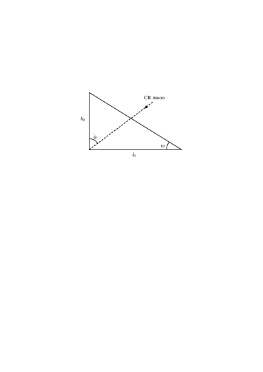
Figure 1: Geometry and slant depth of PUSHEP site.

The triangle nature of site and the slant depth $X(\theta)$ are shown in Fig. 1. For the rock density $\varrho$ we adopt here value $2.72$ g/cm³. The column depth $h(\theta)$ related to the slant depth, $h(\theta)=\varrho X(\theta)$, varies between $h_{\rm min}\simeq 3.0\cdot 10^{5}$ g$\cdot$cm^-2 ($3$ km w. e.) that corresponds to $\cos\theta_{\rm m}\simeq 0.85$ and $h_{\rm max}\simeq 5.71\cdot 10^{5}$ g$\cdot$cm^-2 ($5.71$ km w. e.) near horizontal. Near vertical direction column depth is about 3.54 km w. e.

II.2 Parameterization of the conventional muon spectrum at sea level

The surface muon flux is rather well measured up to TeV and can be described by different analytical formulae taking into account the zenith-angle dependence. Here we list some of them which were used in present calculations. First of all we use Gaisser’s muon flux parameterization gai ; gaisser04 (in inits of $\rm{cm}^{-2}\rm s^{-1}\rm{sr}^{-1}\rm{GeV}^{-1}$)

$$\phi^{\rm\pi,K}_{\mu}(E_{\mu})=0.14E_{\mu}^{-2.7}\left[\frac{1}{1+1.1(E_{\mu}/115{\rm GeV})\cos\theta}+\frac{0.054}{1+1.1(E_{\mu}/850{\rm GeV})\cos\theta}\right].$$ (2)

For our purpose we work with a modified muon flux formula obtained by Tang et al. tang .

Next parameterization of the conventinal muon flux we use here is that by Bugaev et al. bug98 for vertical direction:

$$\phi^{\rm\pi,K}_{\mu}(p_{\mu},0^{\circ})=Cp_{\mu}^{-(\gamma_{0}+\gamma_{1}z+\gamma_{2}z^{2}+\gamma_{3}z^{3})}\,,\ \rm{cm}^{-2}\rm s^{-1}\rm{sr}^{-1}\rm{(GeV/c)}^{-1},$$ (3)

where $z=\log_{10}(p_{\mu}/1~{}\rm{GeV/c})$. Values of parameters in Eq. (3) are listed in Table 1 for different momentum ranges. The muon energy spectrum is $\phi^{\rm\pi,K}_{\mu}(E,\theta)=(E_{\mu}/p_{\mu})\,\phi^{\rm\pi,K}_{\mu}(p_{\mu},\theta)$.

Table 1: Parameters in Eq. (3) for the vertical energy spectrum of conventional muons at sea level.

Momentum range, GeV/c	$C$, (cm 2s  sr  GeV/c)-1	$\gamma_{0}$	$\gamma_{1}$	$\gamma_{2}$	$\gamma_{3}$
$1.0-927.65$	$2.950\times 10^{-3}$	0.3061	1.2743	-0.2630	0.0252
$927.65-1587.8$	$1.781\times 10^{-2}$	1.7910	0.3040	0	0
$1587.8-4.1625\times 10^{5}$	$14.35$	3.6720	0	0	0
$>4.1625\times 10^{5}$	$10^{3}$	4.0	0	0	0

For inclined directions we use zenith-angle dependence given in Ref. tanya (see also ts ). As the third parameterization of the atmospheric muon flux we use the formula given in Ref. reyna .

II.3 Prompt muon contribution

Atmospheric prompt muon flux predictions are reviewed in Refs. bug89 ; costa01 . Ratios of the differential energy spectra of muons at sea level originated from charmed particle decays to that of ($\pi,\,K$)-decays (conventional muons) calculated for a variety of charm production models are shown in Fig. 2 (see also misaki ). Here PRS stands for the model prs , GGV for  ggv2 , RQPM and QGSM for bug89 ; bug98 , and VZ for Volkova and Zatsepin vz ). Among them we dwell below on quark-gluon string model (QGSM), as a sample of phenomenological nonperturbative approach, and also on some of models based on perturbative QCD computations, GGV ggv2 and GBW gbw .

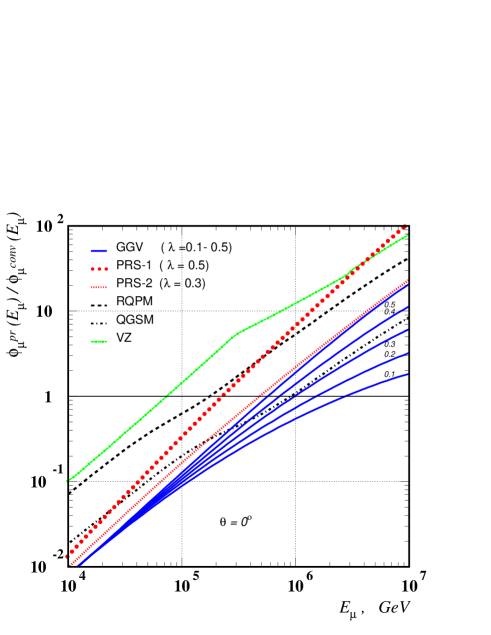
Figure 2: Ratio of the prompt muon flux to the conventional one at ground level.

Gelmini, Gondolo and Varieschi (GGV) ggv2 have included NLO corrections for the charm production with $xg(x)\sim x^{-\lambda},$ ($\lambda$ varying in the range $0-0.5$). These results obey the following parameterization for the sea-level muon fluxes (see also misaki ):

$$\phi^{\rm GGV}_{\mu}(E_{\mu})=A\left(\frac{E_{\mu}}{1~{}\rm{GeV}}\right)^{-(a+by+cy^{2}+dy^{3})},\ \rm{cm}^{-2}\rm s^{-1}\rm{sr}^{-1}\rm{GeV}^{-1}.$$ (4)

where $y=\log_{10}(E_{\mu}/1~{}\rm{GeV})$. The parameters are given in the Table 2. We choose two representative sets corresponding to $\lambda=0.1$ (GGV01) and $\lambda=0.5$ (GGV05).

Table 2: GGV parameters for the prompt muon fluxes.

Model	A, cm-2s-1sr-1GeV${}^{-1}\$	a	b	c	d
GGV01	$3.12\times 10^{-6}$	2.70	-0.095	$1.49\times 10^{-2}$	$-0.2148\times 10^{-3}$
GGV05	$0.58\times 10^{-6}$	1.84	0.257	$-4.05\times 10^{-2}$	$2.455\times 10^{-3}$

QGSM flux parameterization (that is valid for $\theta\lesssim 80^{\circ}$) may be written bug89 as

$$\phi^{\rm QGSM}_{\mu}(E_{\mu})=1.09\cdot 10^{-18}\left(\frac{E_{\mu}}{100\,\rm{TeV}}\right)^{-3.02}\left[1+\left(\frac{E_{\mu}}{100\,\rm{TeV}}\right)^{-2.02}\right]^{-0.165},\ \rm{cm}^{-2}\rm s^{-1}\rm{sr}^{-1}\rm{GeV}^{-1}.$$ (5)

As last representative model, we consider flux calculation within the saturation model proposed by Golec-Biernat and Wuthsoff gbw . For this model, we consider two cases mp ): GBW1, where the protons are taken to be the primary, and GBW2, where we include the effect of heavy elements also. The sea level prompt muon flux due to GBW1 and GBW2 can be parameterized as Eq. (6) and Eq. (7) respectively:

$$\phi^{\rm GBW1}_{\mu}(E_{\mu})=2.35\cdot 10^{-8}\left(\frac{E_{\mu}}{1~{}\rm{GeV}}\right)^{-2.17145-0.04984y},\ \rm{cm}^{-2}\rm s^{-1}\rm{sr}^{-1}\rm{GeV}^{-1},$$ (6)

$$\phi^{\rm GBW2}_{\mu}(E_{\mu})=1.09\cdot 10^{-8}\left(\frac{E_{\mu}}{1~{}\rm{GeV}}\right)^{-1.79371-0.10873y},\ \rm{cm}^{-2}\rm s^{-1}\rm{sr}^{-1}\rm{GeV}^{-1}.$$ (7)

These two cases are different in nature, with the expectation that GBW2 should lead to a decreased muon flux at higher energies.

II.4 Method to calculate the muon flux under thick layer of the rock

In these computations we base on the semianalytical method for the solution of muon transport equation stated in Ref. nsb94 (see also  bug98 ; ts ). The method allows to consider real atmospheric muon spectrum and the energy behavior of discrete energy loss spectra due to radiative and photonuclear interactions of muons in matter. Only ionization energy loss of muons are treated as continuous one. The method provides effective tool to compute the energy spectra of cosmic-ray muons at large depths of homogeneous media. The benefits of this approach are to carry out verifications of the primary CR spectrum and composition, charm production models, models of the photonuclear interaction with high performance and good precision. This enables to estimate the sea-level muon spectrum using the data of underground/underwater measurements evading the difficult inverse scattering problem.

III Expected muon flux at the depth of PUSHEP site

Zenith-angle distributions of the conventional muon flux calculated for five values of the minimal energy of muons in the range $10$–$10^{5}$ GeV at depth $1.3$ km of INO detector are shown in Fig. 3. Here solid lines represent computations for the surface muon spectrum bug98 by Bugaev et al. with usage of the angle dependence obtained in Ref. tanya (see also ts ). Dashed lines, almost superimposed on solid ones but near horizontal directions, show results for the spectrum by Tang et al. tang whereas dotted ones show that for the spectrum by Reyna reyna . The geometry of the INO site is reflected in the flat shape of the underock distribution(see Fig. 1).

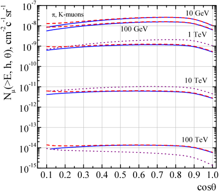
Figure 3: Angle distributions of the conventional muons near the INO detector.

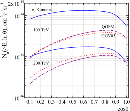
Figure 4: Zenith-angle distributions of atmospheric muons at $100$ and $200$ TeV.

Zenith-angle dependence of the conventional and prompt muon fluxes at the INO depth are shown in Figs. 4 and 5. In Fig. 4 are shown the prompt muon flux at muon energy above $100$ and $200$ TeV calculated with QGSM charm production cross sections (dash-dotted lines) and that of GGV models. For muon energy above $500$ TeV we also plot predictions obtained for GBW model (dashes line in Fig. 5). As one may clearly observe in Fig. 5, measurement of high muon flux near the vertical at INO depth could allow to discriminate between GGV01($\lambda=0.1$) model and GGV05($\lambda=0.5$) or QGSM one. While the GBW prompt muon flux is unlikely to be observed at 500 TeV.

Differential muon spectra (left panel) at INO depth and integral ones (right panel) are presented in Fig. 6 for $\cos\theta=0.7$, where solid line shows the conventional muon flux obtained with usage of Bugaev et al. boundary spectrum and circles denote that for Gaisser’s spectrum. We can see in Fig. 6 that crossover energy for the conventional muon flux and the GGV05 prompt one is about $300$ TeV, therefore it seems that more suitable for the prompt muon identification is to analyse the zenith-angle dependence of high-energy muon flux (see Fig. 4).

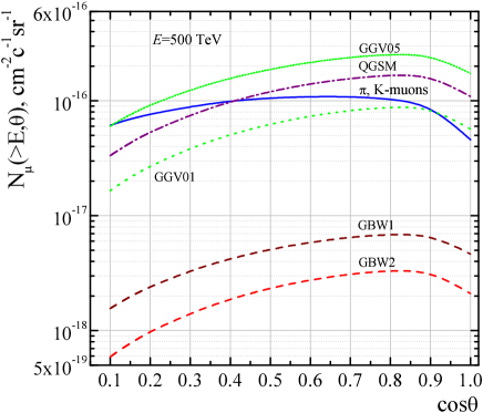
Figure 5: Very high-energy zenith-angle distributions of atmospheric muons.

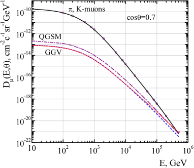
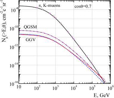
Figure 6: Energy spectra of the atmospheric muons near the INO detector.

Number of the muon events per steradian per year expected at INO detector near direction $\cos\theta=0.7$ is presented in Table 3 (see details in Ref. gp ).

Table 3: Number of the muon events per steradian per year expected at INO detector.

$E_{\mu}$, TeV	conv.	GGV01	GGV05	QGSM	$R_{c}^{\rm GGV01}$	$R_{c}^{\rm GGV05}$	$R_{c}^{\rm QGSM}$
$10$	$60097$	$1235$	$1353$	$3037$	$0.02$	$0.022$	$0.05$
$50$	$832$	$73$	$105$	$159$	$0.087$	$0.126$	$0.19$
$100$	$132$	$20$	$34$	$41$	$0.15$	$0.258$	$0.31$
$200$	$20$	$5.0$	$10$	$10$	$0.25$	$0.50$	$0.50$
$300$	$6.0$	$2.0$	$5.0$	$4.0$	$0.33$	$0.83$	$0.66$
$400$	$2.6$	$1.0$	$2.6$	$2.2$	$0.38$	$1.0$	$0.85$
$500$	$1.4$	$0.6$	$1.6$	$1.2$	$0.43$	$1.14$	$0.86$

Last three columns in Table 3 represent the ratio of the conventional muon flux to the prompt muon one due to three charm production models, GGV01, GGV05 and QGSM, respectively.

IV Summary

The shape of zenith-angle distributions of conventional muons is nearly flat (see Figs. 3–5). Therefore muons arriving at the detector close to vertical directions are more favorable to measure the prompt muon flux. The prompt muon contribution to the atmospheric muon flux increases with energy because of lower value of the energy spectrum index. The “crossover” energy, $E_{c}$, at which the prompt muon flux becomes equal to the conventional one, depends strongly on the charm production model. Following numbers can illustrate (see Fig. 2) the $E_{c}$ at INO depth for some of charm hadroproduction models: $E_{c}^{\rm GGV05}\simeq 250$ TeV, $E_{c}^{\rm QGSM}\simeq 300$ TeV, $E_{c}^{\rm GGV01}\simeq 600$ TeV.

From the Table 3 we can see that prompt muon flux contribution due to GGV01 model, for example, may differs from that for the GGV051 model (or QGSM) by factor 2 at $E_{\mu}>200$ TeV. In other words, expected number of muon events inside the INO detector may increase by $50$ % at the energy above $200$ TeV if GGV05 or QGSM predictions are reasonable.

V Acknowledgements

The work of S.P. was supported by the Ministerio de Educación y Ciencia under Proyecto Nacional FPA2006-01105, and also by the Comunidad de Madrid under Proyecto HEPHACOS, Ayuda de I+D S-0505/ESP-0346. The author S.P would like to thank Indumati for providing valuable information regarding INO experiment. We thank Pankaj jain for careful reading the manuscript. S. Sinegovsky acknowledges the support by Federal Programme ”Leading Scientific Schools of Russian Federation”, grant NSh-5362.2006.2.

References

- (1) T. K. Gaisser, Cosmic Rays and Particle Physics, (Cambridge University Press, Cambridge) 1990;
- (2) M. Nagano and A. A. Watson, Rev. Mod. Phys. 72, 689 (2000); P. Bhattacharjee and G. Sigl, Phys. Reports 327, 109 (2000); Astropart. Phys. 16, 373 (2000).
-
(3)
K.-H. Kampert et al. (KASCADE Collaboration), Proceedings of the 26th ICRC 26, Salt Lake City, Utah, 1999, edited by D. Kieda, M. Solomon and B. Dingus, Vol. 3, p. 159 (OG.1.2.11).
Acta Phys.Polon. B 35 1799, (2004) [astro-ph/0405608]; M. Aglietta et al.(EAS-TOP Collaboration and MACRO Collaboration), Astropart. Phys. 20, 641 (2004). - (4) S. Ostapchenko, hep-ph/0612068; R. Engel, Nucl. Phys. Proc. Suppl. 151, 437 (2006).
- (5) P. Lipari, Astropart. Phys. 1 195 (1993).
- (6) E. V. Bugaev et al., Nuovo Cim. C 12, 41 (1989).
- (7) C. G. S. Costa, Astropart. Phys. 16, 193 (2001).
- (8) M. Thunman, G. Ingelman and P. Gondolo, Astropart. Phys. 5, 309 (1996).
- (9) L. Pasquali, M. H. Reno and I. Sarcevic, Phys. Rev. D59, 034020 (1999).
- (10) G. Gelmini, P. Gondolo and G. Varieschi Phys. Rev. D61, 036005 (2000); Phys. Rev. D61, 056011 (2000); Phys. Rev. D 67, 017301 (2003).
- (11) M. Aglietta et. al. (LVD Collaboration), Phys. Rev. D60, 112001 (1999); M. Nagano et. al., Journ. of Physics G: Nucl. Phys. 12, 69 (1986); P. Desiati et. al. (AMANDA Collaboration), Proceedings of the 28th ICRC, Tsukuba, Japan, 2003, HE 2.1, p. 1373; http://amanda.berkeley.edu/
- (12) Raj Gandhi and Sukanta Panda, JCAP 0607, 011 (2006); hep-ph/0512179.
- (13) Namit Mahajan and Sukanta Panda, hep-ph/0701003.
- (14) K. Golec-Biernat and M. Wusthoff, Phys. Rev. D 59, 014017 (1999); K. Golec-Biernat and M. Wusthoff, Phys. Rev. D 60, 114023 (1999).
- (15) M. Sajjad Athar et al. (INO Collaboration), India-based Neutrino Observatory: Project Report. Volume I. INO-2006-01, May 2006. 233pp. http://www.imsc.res.in/ ino/OpenReports/INOReport.pdf
- (16) T. K. Gaisser and T. Stanev, Phys. Lett. B 592, 228 (2004).
- (17) A. Tang et al., Phys. Rev. D 74, 053007 (2006)
- (18) E. V. Bugaev et al. Phys. Rev. D 58, 054001 (1998); hep-ph/9803488.
- (19) T. S. Sinegovskaya, Proceedings of the 2nd Baikal School on Fundamental Physics “Interaction of radiation and fields with matter”, Irkutsk, Russia, 1999, edited by Yu. N. Denisyuk and A. N. Malov (Irkutsk University, 1999) Vol. 2, p.598 (in Russian).
- (20) T. S. Sinegovskaya and S. I. Sinegovsky, Phys. Rev. D 63, 096004 (2001); hep-ph/0007234.
- (21) D. Reyna, hep-ph/0604145v2.
- (22) A. Misaki et al., J. Phys. G: Nucl. Part. Phys. 29, 387 (2003).
- (23) L. V. Volkova, G. T. Zatsepin, Phys. Atom. Nucl. 63, 1050 (2000); Phys. Atom. Nucl. 64, 266 (2001);
- (24) V. A. Naumov, S. I. Sinegovsky and E. V. Bugaev, Phys. Atom. Nucl. 57, 412 (1994); hep-ph/9301263.