On the evolution of clustering of 24$\mu$m-selected galaxies.

Abstract

This paper investigates the clustering properties of a complete sample of 1041 24$\mu$m-selected sources brighter than $F_{24\mu\rm m}=400\mu$Jy in the overlapping region between the SWIRE and UKIDSS UDS surveys. With the help of photometric redshift determinations we have concentrated on the two interval ranges $z=[0.6-1.2]$ (low-z sample) and $z\geq 1.6$ (high-z sample) as it is in these regions were we expect the mid-IR population to be dominated by intense dust-enshrouded activity such as star formation and black hole accretion. Investigations of the angular correlation function produce an amplitude $A\sim 0.010$ for the high-z sample and $A\sim 0.0055$ for the low-z one. The corresponding correlation lengths are $r_{0}=15.9^{+2.9}_{-3.4}$ Mpc and $r_{0}=8.5^{+1.5}_{-1.8}$ Mpc, showing that the high-z population is more strongly clustered. Comparisons with physical models for the formation and evolution of large-scale structure reveal that the high-z sources are exclusively associated with very massive ($M\mathrel{\hbox to0.0pt{\lower 3.0pt\hbox{$\sim$}\hss}\raise 2.0pt\hbox{$>$}}10^{13}M_{\odot}$) haloes, comparable to those which locally host groups-to-clusters of galaxies, and are very common within such (rare) structures. Conversely, lower-z galaxies are found to reside in smaller halos ($M_{\rm min}\sim 10^{12}M_{\odot}$) and to be very rare in such systems. On the other hand, mid-IR photometry shows that the low-z and high-z samples include similar objects and probe a similar mixture of AGN and star-forming galaxies. While recent studies have determined a strong evolution of the 24$\mu$m luminosity function between $z\sim 2$ and $z\sim 0$, they cannot provide information on the physical nature of such an evolution. Our clustering results instead indicate that this is due to the presence of different populations of objects inhabiting different structures, as active systems at $z\mathrel{\hbox to0.0pt{\lower 3.0pt\hbox{$\sim$}\hss}\raise 2.0pt\hbox{$<$}}1.5$ are found to be exclusively associated with low-mass galaxies, while very massive sources appear to have concluded their active phase before this epoch. Finally, we note that the small-scale clustering data seem to require steep ($\rho\propto r^{-3}$) profiles for the distribution of galaxies within their halos. This is suggestive of close encounters and/or mergers which could strongly favour both AGN and star-formation activity.

1 Introduction

Understanding the assembly history of massive spheroidal galaxies is a key issue for galaxy formation models. The “naive” expectation from the canonical hierarchical merging scenario, that proved to be remarkably successful in explaining many aspects of large-scale structure formation, is that massive galaxies generally form late and over a long period of time as the result of many mergers of smaller haloes. On the other hand, there is quite extensive evidence that massive galaxies may form at high redshifts and on short timescales (see, e.g. Cimatti et al. 2004; Fontana et al. 2004; Glazebrook et al. 2004; Treu et al. 2005; Saracco et al. 2006; Bundy et al. 2006; McLure et al. 2006), while the sites of active star formation shift to lower mass systems at later epochs, a pattern referred to as ”downsizing” (Cowie et al. 1996; Heavens et al. 2004). In order to reconcile the observational evidence that stellar populations in large spheroidal galaxies are old and essentially coeval (Ellis et al. 1997; Holden et al. 2005) with the hierarchical merging scenario, the possibility of mergers of evolved sub-units (“dry mergers”) has been introduced (van Dokkum et al. 2005; Naab et al. 2006). This mechanism is however strongly disfavoured by studies on the evolution of the stellar mass function (Bundy et al. 2006).

Key information, complementary to optical/IR data, has come from sub-millimeter surveys (Hughes et al. 1998; Eales et al. 2000; Scott et al. 2002; Knudsen et al. 2006; Coppin et al. 2006) which have found a large population of luminous sources at substantial redshifts (Chapman et al. 2005). However, the interpretation of this class of objects is still controversial (e.g. Granato et al. 2004; Kaviani et al. 2003; Baugh et al. 2005). The heart of the problem are the masses of the objects: a large fraction of present day massive galaxies already assembled at $z\sim 2-3$ would be extremely challenging for the standard view of a merging-driven growth. Measurements of clustering amplitudes are a unique tool to estimate halo masses at high $z$, but complete samples comprising at least several hundred of sources are necessary.

Recently, Magliocchetti et al. (2007) have reported evidence for strong clustering for $\sim 800$ optically very faint ($R>25.5$), $F_{24\mu\rm m}\geq 0.35$ mJy sources obtained from the Spitzer first cosmological survey (First Look Survey – FLS; Fadda et al. 2006). Both the clustering properties and the counts of such sources are consistent with them being very massive proto-spheroidal galaxies in the process of forming most of their stars. Furthermore, by assuming a medium redshift $z\sim 2$, their comoving number density appears to be much higher than what expected from most semi-analytic models.

The Magliocchetti et al. (2007) work however suffers from the lack of information on the redshift distribution of the optically faint Spitzer-selected sources and has to rely on models based on both template spectral energy distributions and on theoretical investigations of the issue of galaxy formation and evolution in order to go from the observed projected clustering signal to the more meaningful results in real space.

The optical-to-mid-IR depth of the UKIDSS data allows us to overcome this problem. Photometric estimates for the overwhelming majority ($\sim 97$%) of 24$\mu$m-selected sources are now available (Cirasuolo et al. 2007). Furthermore, despite the somehow poor statistics, the redshift information can also allow us for the first time to compare the clustering signal of similar sources at different epochs so to investigate possible differences and evolution in their large-scale properties. To this aim, we will concentrate on two samples, the first one which includes galaxies in the $z=[0.6-1.2]$ range, and a second one made by sources with $z\mathrel{\hbox to0.0pt{\lower 3.0pt\hbox{$\sim$}\hss}\raise 2.0pt\hbox{$>$}}1.6$. Diagnostics based on mid-IR photometry indicate that these two samples are likely made by a very similar mixture of active star-forming galaxies and AGN.

The layout of the paper is as follows: In § 2 we describe the parent catalogue and the sample selection. In §3.1 we derive the two point angular correlation function, while in §3.2 we present the results for the spatial clustering properties of the sources in exam. §4 discusses the implications of the clustering results on the source properties, and in particular for what concerns their halo masses and number density. Our main conclusions are summarized in § 5.

Throughout this work we adopt a flat cosmology with $\Omega_{m}=0.3$ and $\Omega_{\Lambda}=0.7$, a present-day value of the Hubble parameter in units of $100$ km/s/Mpc $h=0.7$, and rms density fluctuations within a sphere of $8h^{-1}$ Mpc radius $\sigma_{8}=0.8$ (Spergel et al. 2003).

2 Sample Selection

For this work we used the Spitzer wide-area infrared extragalactic (SWIRE) survey (Lonsdale et al. 2003; 2004) to select sources with fluxes at 24 $\mu$m brighter than 400 $\mu$Jy ($5\sigma$ completeness) in the XMM-LSS field (Surace et al. 2005). In order to obtain multi-wavelength information and accurate redshift estimates for these sources we limited our analysis to the region of the SWIRE survey which overlaps with the 0.7 square degrees covered by the UKIDSS Ultra Deep Survey (UDS - Lawrence et al. 2006) and Subaru imaging (Sekiguchi et al. 2005; Furusawa et al. in preparation). The 5 overlapping Subaru Suprime-Cam pointings provide broad band photometry in the $BVRi^{\prime}z^{\prime}$ filters to typical $5\sigma$ depths of $B=27.5$, $V=26.7$, $R=27.0$, $i^{\prime}=26.8$ and $z^{\prime}=25.9$ (within a $2$-arcsec diameter aperture). The UDS is the deepest of the five surveys that constitute the UKIDSS survey (Lawrence et al. 2006) and for this work we used $J$ and $K$-band imaging from the first data release with a $5\sigma$ depth of $J_{AB}=23.5$ and $K_{AB}=23.5$ (Warren et al. 2007). Finally, the SWIRE survey also provides Spitzer-IRAC measurements at 3.6, 4.5, 5.8 and 8$\mu$m (Surace et al. 2005).

Within the overlapping region between SWIRE and UDS we isolated 1184 sources with $F_{24\mu\rm m}\geq 400\mu$Jy, out of which 1041 have a reliable optical and/or near-infrared counterpart. We take these objects as our working sample, UDS-SWIRE hereafter. As extensively described in Cirasuolo et al. (2007), photometric redshifts for these sources have been computed by fitting the observed photometry (9 broad bands from 0.4 to 4.5$\mu m$) with both synthetic (Bruzual & Charlot 2003) and empirical (Coleman, Wu & Weedman 1980; Kinney et al. 1996; Mignoli et al. 2005) galaxy templates, by using the public package HYPERZ (Bolzonella, Miralles & Pelló 2000). Comparisons with spectroscopic redshifts available in the field show the good accuracy of the photometric redshifts with a $\Delta z/(1+z)\simeq 0.05$ over the redshift range $0<z<6$ (Cirasuolo et al. 2007).
The redshift distribution $N(z)$ for our 24$\mu$m sources is shown by the dotted line in Figure 1. As it is possible to appreciate from the Figure, the objects included in the UDS, $F_{24\mu\rm m}\geq 400\mu$Jy sample are found up to redshifts $z\sim 3.5$.

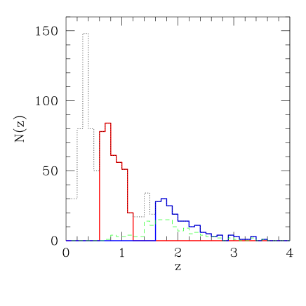
Figure 1: Photometric redshift distribution of sources in the UDS-SWIRE, $F_{24\mu\rm m}\geq 400\mu$Jy sample (thin dotted line). The two thick solid lines highlight the redshift intervals covered by the high-z (blue) and low-z (red) samples. For comparison, the (green) dashed line indicates the redshift distribution of all $F_{24\mu\rm m}\geq 400\mu$Jy sources fainter than $R=24.5$. No redshift cut was performed on this last sample.

In order to investigate possible evolutionary features of the large-scale structure as traced by these objects, we have concentrated on two sub-samples: a first one which includes both sources with redshifts above 1.6 and those without an optical or K-band identification (hereafter called the high-z sample) and a second one with objects within $z=0.6$ and $z=1.2$ (hereafter called the low-z sample). There are a number of reasons for the above choice. $z\sim 1.6$ is in fact the redshift at which the strong spectral PAH feature centred at 7.7$\mu$m – indicative of a very intense star-forming activity – enters the 24$\mu$m band. The high-z sample is therefore expected to include a relevant fraction of galaxies undergoing an intense phase of dust-enshrouded stellar formation. Furthermore, recent studies have proved that a strong 24$\mu$m emission combined with a very faint or no optical detection most likely originates from obscured star-forming galaxies at redshifts between about 1.6 and 2.7 (see e.g. Yan et al. 2005; 2007; Houck et al. 2005). On the other hand, results both based on IRS spectroscopy and on diagnostics of the ratio between 8$\mu$m and 24$\mu$m fluxes, have inferred a fraction of $z\sim 2$ obscured AGN brighter than our chosen 24$\mu$m flux limit of about 30%, figure which rapidly increases to $\sim 100$% at the highest 24$\mu$m fluxes (see e.g. Brand 2006; Magliocchetti et al. 2007). The counts presented in the right-hand panel of Figure 2 seem to confirm this expectation ($\sim 65$% candidate starburst galaxies on the basis of their $F_{8\mu\rm m}/F_{24\mu\rm m}<0.1$ ratios, with the remaining $\sim 35$% being made of candidate AGN-dominated objects).

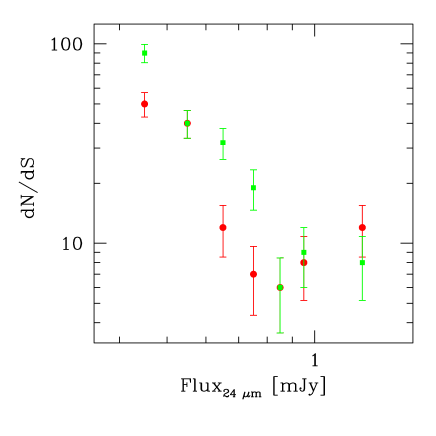
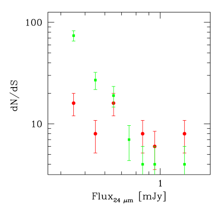
Figure 2: Differential number counts for candidate star-forming galaxies ($F_{8\mu\rm m}/F_{24\mu\rm m}<0.1$; green squares) and candidate AGN-dominated sources ($F_{8\mu\rm m}/F_{24\mu\rm m}\geq 0.1$; red circles) in the low-z (left-hand panel) and high-z (right-hand panel) samples.

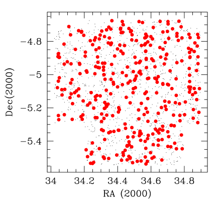
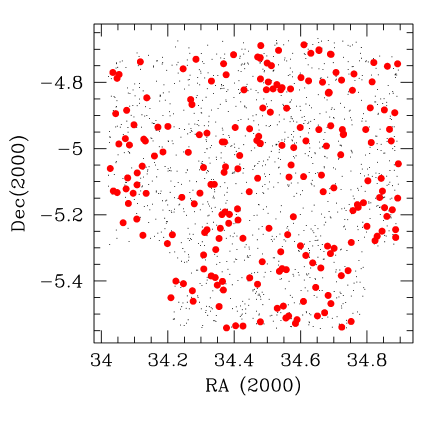
Figure 3: Sky distribution of UDS-SWIRE, $F_{24\mu\rm m}\geq 400\mu$Jy sources (small dots). The filled (red) circles in the left-hand panel illustrate the 350 objects included in the redshift interval $z=[0.6-1.2]$, while those in the right-hand panel represent the 210 sources with either $z>1.6$ or no optical or near-IR identification.

The low-z sample is also expected to probe a substantial fraction of obscured star-forming galaxies and AGN, albeit with lower intrinsic luminosities since we are dealing with a flux-limited survey. The $24\mu\rm m$ counts presented in the left-hand panel of Figure 2 are remarkably similar to those obtained for the high-z sample ($\sim 60$% and $\sim 40$% respectively for candidate starburst galaxies and candidate AGN-dominated objects; we note that the lower limit of $z\sim 0.6$ adopted for the low-z sample corresponds to the lowest redshift at which a meaningful distinction between AGN-powered and SF-dominated sources as based on the ratio between $F_{8\mu\rm m}$ and $F_{24\mu\rm m}$ fluxes can be made given the spectral properties of intense star-forming galaxies in the mid-IR). Furthermore, from recent multi-photometry studies which extend from the optical to the X-ray band, it seems that $z\sim 1$ corresponds to the ’bulk’ of obscured AGN activity (see e.g. Pozzi et al. 2007). A comparative analysis of the two samples would then allow to investigate any redshift evolution in the large-scale properties of these sources and, if present, find an evolutionary connection between objects in the low-z and high-z samples.

The high-z sample includes 210 sources, 28 of which do not have an optical counterpart. The redshift distribution of the objects with assigned photo-z closely resembles that of $R\geq 24.5$, 24$\mu$m-selected galaxies (cfr. Figure 1), showing once again that optically-faint sources selected at 24$\mu$m most likely reside at redshifts $z>1.6$. The projected distribution onto the sky of the high-z sources is shown by the filled (red) circles on the right-hand side of Figure 3. Small dots indicate the positions of all $F_{24\mu\rm m}\geq 400\mu$Jy UDS-SWIRE objects.
By making use of the redshift distribution shown in Figure 1, and assuming that the $N(z)$ of optically obscured sources follows that of galaxies with estimated redshift, we find that the average redshift for the above sample is $<z>=2.02$, its median is $z_{\rm med}=1.93$, and the mean comoving number density of such sources is $\bar{n}_{G}=(2.5\pm 0.3)\cdot 10^{-5}$ Mpc^-3, number which decreases to $\bar{n}_{G}=(2.2\pm 0.3)\cdot 10^{-5}$ Mpc^-3 if one only includes objects with redshifts. The errors associated to the above quantities represent the 2$\sigma$ confidence level as derived from Poisson statistics. Estimates of the number density at $z\sim 2$ might be very tricky due to joint effect of the cosmological evolution of the sources under examination and to the large variance of the observed 24$\mu$m SED in that redshift range. This is why, for a safety check, we have also repeated our calculations of $\bar{n}_{G}$ by simply considering a redshift box extending from $z=1.6$ to $z=2.5$. The result is virtually identical to that quoted above both by including and excluding galaxies with no redshift information and also very similar to that obtained by extrapolating the $z\sim 2$ Caputi et al. (2007; cfr. their Figure 8) Luminosity Function for 24$\mu$m-selected galaxies brighter than $\nu L_{\nu}\simeq 10^{11.9}L_{\odot}$, where the limiting luminosity has been calculated for $F_{24\mu\rm m}=0.4$ mJy by following an Arp220-like Spectral Energy Distribution, indicative of galaxies undergoing intense star-formation which we expect (cfr. earlier in this section and also Figure 2) to dominate our sample.

The low-z sample instead contains 350 sources. Their sky distribution is represented by the filled (red) circles on the left-hand side of Figure 3. The average redshift of the sample is found to be $<z>=0.79$, its median $z_{\rm med}=0.84$, and the comoving number density of these sources is $\bar{n}_{G}=(9.9\pm 1.0)\cdot 10^{-5}$ Mpc^-3. Even in this case, the number density is in excellent agreement with the findings of Caputi et al. (2007) for their $z\sim 1$ sources with $\nu L_{\nu}\mathrel{\hbox to0.0pt{\lower 3.0pt\hbox{$\sim$}\hss}\raise 2.0pt\hbox{$>$}}10^{11.3}L_{\odot}$, where $\nu L_{\nu}$ was calculated as indicated before. The most relevant properties for the high-z and low-z samples are summarized in Table 2.

3 Clustering properties

3.1 The Angular Correlation Function

The angular two-point correlation function $w(\theta)$ gives the excess probability, with respect to a random Poisson distribution, of finding two sources in the solid angles $\delta\Omega_{1}$ $\delta\Omega_{2}$ separated by an angle $\theta$. In practice, $w(\theta)$ is obtained by comparing the actual source distribution with a catalogue of randomly distributed objects subject to the same mask constraints as the real data. We chose to use the estimator (Hamilton 1993)

$$w(\theta)=4\times\frac{DD\cdot RR}{(DR)^{2}}-1,$$ (1)

where $DD$, $RR$ and $DR$ are the number of data-data, random-random and data-random pairs separated by a distance $\theta$.

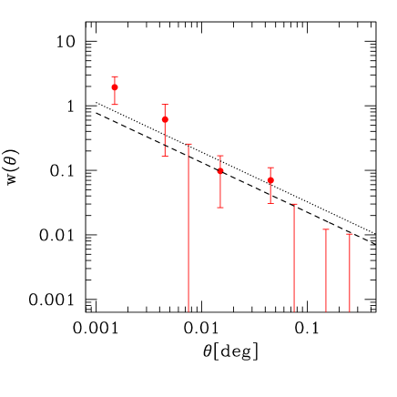
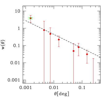
Figure 4: Angular correlation function $w(\theta)$ for the low-z (left-hand panel), and high-z (right-hand panel) samples. The dashed lines show the best power-law fits to the data, while the dotted line in the left-hand panel indicates the variation in the best fit obtained by considering the $w(\theta)+1\sigma$ values at those scales where $w(\theta)$ is negative as mere upper limits. The two horizontal (green) dashes in the plot for the high-z sample represent the small-scale variation of $w(\theta)$ derived by either including or excluding the pair of sources whose distance from each other is $<5.4^{\prime\prime}$ (see text for details).

The two considered UDS-SWIRE samples have an estimated 5$\sigma$ flux completeness $F_{24\mu\rm m}\geq 400\mu$Jy. Furthermore, since the whole UDS area was uniformly observed by Spitzer/MIPS, we only had to mask out those (few) portions of the sky contaminated by the presence of bright stars. Random catalogues covering the whole surveyed area minus the bright star regions and with twenty times as many objects as the real data sets were then generated for both the high-z and low-z samples. $w(\theta)$ in eq. (1) was then estimated in the angular range $10^{-3}\mathrel{\hbox to0.0pt{\lower 3.0pt\hbox{$\sim$}\hss}\raise 2.0pt\hbox{$<$}}\theta\mathrel{\hbox to0.0pt{\lower 3.0pt\hbox{$\sim$}\hss}\raise 2.0pt\hbox{$<$}}0.3$ degrees. The upper limit is determined by the geometry of UDS, and corresponds to about half of the maximum scale probed by the survey.

Figure 4 presents our results for the two low-z (left-hand panel) and high-z (right-hand panel) samples, while Table 1 reports the $w(\theta$) values as a function of angular scale in both cases. The error bars show Poisson estimates for the points. Since the distribution is clustered, these estimates only provide a lower limit to the uncertainties. However, it can be shown that over the considered range of angular scales this estimate is close to those obtained from bootstrap resampling (e.g. Willumsen, Freudling & Da Costa, 1997).

Particular attention was devoted to the issue of close pairs. In fact, the points on the top left-hand corners of both $w(\theta)$ estimates correspond to angular scales close to the 5.4^′′ resolution of the 24$\mu$m Spitzer channel and therefore could be affected by source confusion. However, since optical and near-infrared images for these sources have a much better resolution ($\sim$0.8^′′), we can use this information and consider as ’good’ pairs all those made of galaxies which are identified in the Subaru/UDS images, while we regard as potentially spurious those made of galaxies without such optical/near-IR counterparts. For the low-z sample, there are 11 pairs with distances between 0.001 and 0.003 degrees. Of these, only one was found to be closer than 5.4^′′ and both IRAC and R-band photometry indicate that we are dealing with two distinct sources. 10 close (i.e. again with distances between 0.001 and 0.003 degrees) pairs are instead found in the high-z sample. Of these, only one is at a distance below 5.4^′′. Unfortunately, the two sources of this pair are unidentified both in the optical and in the near-IR bands, and so the pair has to be considered as spurious.

The angular correlation function for the high-z sample was then computed by both including and excluding the possibly spurious pair. The small-scale ($\theta\sim 0.0015^{\circ}$) results are shown by the two horizontal dashes in the right-hand panel of Figure 4. The filled circle represents their average. As it is possible to see, the $w(\theta)$ variation caused by the eventual presence of the spurious pair is almost negligible, and surely smaller than the error associated to the determination of $w(\theta)$. Nevertheless, in the following we will use as the ’best’ small-scale point, that obtained as the average of the two estimates and the associated error will be the sum in quadrature of the Poisson one and of the variation due to the inclusion/exclusion of the pair.

If we then assume a power-law form for $w(\theta)=A\theta^{1-\gamma}$, we can estimate the parameters $A$ and $\gamma$ by using a least-squares fit to the data. Given the large errors on $w$ we choose to fix $\gamma$ to the standard value $\gamma=1.8$. Although somewhat arbitrary, this figure and its assumed lack of dependence on redshift is justified by LSS observations of large enough samples of high redshift sources so to allow for a direct estimate of the slope of $w(\theta)$ at different look back times (e.g. Porciani, Magliocchetti & Norberg 2004; Le Fevre et al. 2005). The small area of the UDS survey introduces a negative bias through the integral constraint, $\int w^{est}d\Omega=0$. We allow for this by fitting to $A\theta^{1-\gamma}-C$, where $C=2.5A$.
The dashed lines in Figure 4a and 4b represent the best power-law fits respectively to the low-z and high-z data. The associated best-fit values for the amplitude are $A^{\rm lz}=[3.8\pm 1.6]\cdot 10^{-3}$ for the low-z sample, and $A^{\rm hz}=[10.0\pm 3.5]\cdot 10^{-3}$ for the high-z sample.

The amplitude for the high-z sample is in good agreement with that obtained by Magliocchetti et al. (2007) by analyzing a sample of $\sim 800$ heavily obscured ($R\geq 25.5$) Spitzer-selected sources from the First Look Survey (FLS, Fadda et al. 2006) with $F_{24\mu\rm m}\geq 0.35$ mJy. This provides us with some confidence that cosmic variance is not a cause for main concern in our analysis of high-z UDS-SWIRE sources. Furthermore, as already noticed by the above authors, in this case $A$ is about four times higher than that derived by Fang et al. (2004) for a sample of IRAC galaxies selected at 8$\mu$m ($A\sim 2.34\cdot 10^{-3}$), and about ten times higher than that obtained by Magliocchetti et al. (2007) for the whole $F_{24\mu\rm m}\geq 0.35$ mJy FLS dataset ($A=[9\pm 2]\cdot 10^{-4}$).

Table 1: Values for the angular correlation function $w(\theta)$ as obtained for the low-z and high-z samples. Error bars are obtained from Poisson statistics.

$\theta$ [Deg]	Low-z sample	High-z sample
0.0015	$1.9\pm 0.9$	$3.8\pm 1.7$
0.0045	$0.6\pm 0.4$	$0.8\pm 1.8$
0.0075	$-0.19\pm 0.25$	$0.5\pm 0.6$
0.0150	$0.10\pm 0.07$	$0.2\pm 0.1$
0.0450	$0.07\pm 0.04$	$0.05\pm 0.08$
0.0750	$-0.004\pm 0.03$	$0.08\pm 0.05$
0.1500	$-0.0004\pm 0.01$	$0.03\pm 0.02$
0.2500	$-0.01\pm 0.01$	$-0.013\pm 0.017$

The case for the low-z sample is more tricky to deal with. The inferred value for the amplitude of its angular correlation function in fact suggests that UDS-SWIRE sources at $z\sim 1$ are sensibly less clustered (about a factor three in angular signal) than higher redshift ones. However, the computed $w(\theta)$ for the low-z sample presents puzzling negative values in four $\theta$ bins which should instead correspond to $w(\theta)>0$. We have re-analyzed the sample a number of times by both varying the bin size and by adopting different prescriptions and dimensions for the random catalogue in the calculation of $w(\theta)$ and we can conclude that the observed negative values for $w(\theta)$ are indeed a real feature of the $z\sim 1$ sample. However, we cannot quantify how much of this trend is affected by poor statistics and/or cosmic variance (for instance, Gilli et al. 2007 find a variation in the number of $z\sim 1$, 24$\mu$m-selected sources brighter than approximately our chosen limit of almost a factor 2 between the two GOODS fields set in the northern and in the southern sky). While we note that also the Gilli et al. (2007) correlation function as estimated at $z\sim 0.7$ for the GOODS South exhibits a dip at scales $\sim 0.2/h$ Mpc which – for the chosen cosmology – correspond to the $\theta\sim 0.008^{\circ}$ bin where we find a negative value for $w(\theta)$, nevertheless caution has to be used when dealing with the four negative $w(\theta)$ figures. This is why we have decided to lower the weight of these points in our $\chi^{2}$ analysis by considering the estimated $w(\theta)+1\sigma$ values (see Table 1) as mere upper limits. The resulting amplitude of the angular correlation function for low-z UDS-SWIRE galaxies in this case is $A^{\rm lz}=5.5^{+1.5}_{-2.0}\cdot 10^{-3}$, about 40 per cent higher than what previously found by including measured data points for $w(\theta)$ at all scales. This is the value which we will adopt throughout the paper and which – though allowing for the large uncertainties – still results to be a factor $\sim$2 lower than that derived from the high-z sample. We will investigate the implications of this result in the following sections.

3.2 Relation to spatial quantities

Table 2: Properties of the two $F_{400\mu\rm m}\geq 400$ mJy samples considered in this work. From left to right the columns show the average redshift $<z>$, the number of sources, the comoving number density $\bar{n}_{G}$ (in $[10^{-5}\>$Mpc${}^{-3}]$ units), the amplitude $A$ of the angular correlation function, the comoving clustering length $r_{0}$ (in Mpc units), the minimum mass $M_{\rm min}^{\rm NFW}$ (in $M_{\odot}$ units) for the dark matter halos, normalization $N_{0}^{\rm NFW}$ and slope of the HON $\alpha^{\rm NFW}$ – all three estimated under the assumption of a NFW profile for the distribution of galaxies within their dark matter halos –, the same quantities evaluated under the assumption of a steeper $\rho\propto r^{-3}$ (PL3) profile, and the large-scale bias $b$.

$<z>$	N	$\bar{n}_{G}$	$A\cdot 10^{-3}$	$r_{0}$	$\rm LogM_{\rm min}^{\rm NFW}$	$\rm LogN_{0}^{\rm NFW}$	$\alpha^{\rm NFW}$	$\rm LogM_{\rm min}^{\rm PL3}$	$\rm LogN_{0}^{\rm PL3}$	$\alpha^{\rm PL3}$	bias
2.02	210	$2.5\pm 0.3$	$10.0\pm 3.5$	$15.9^{+2.9}_{-3.4}$	$12.8^{+0.3}_{-0.3}$	$-0.7^{+0.5}_{-0.5}$	$0.8^{+0.3}_{-0.6}$	$12.8^{+0.4}_{-0.2}$	$-0.7^{+0.5}_{-0.5}$	$0.7^{+0.3}_{-0.5}$	6.17
0.79	350	$9.9\pm 1.0$	$5.5^{+1.5}_{-2.0}$	$8.5^{+1.5}_{-1.8}$	$11.9^{+0.6}_{-0.8}$	$-2.0^{+0.8}_{-0.9}$	$0.8^{+0.1}_{-0.2}$	$11.8^{+0.8}_{-0.8}$	$-2.1^{+1.1}_{-0.9}$	$0.7^{+0.1}_{-0.3}$	1.70

The standard way of relating the angular two-point correlation function $w(\theta)$ to the spatial two-point correlation function $\xi(r,z)$ is by means of the relativistic Limber equation (Peebles, 1980):

$$w(\theta)=2\>\frac{\int_{0}^{\infty}\int_{0}^{\infty}F^{-2}(x)x^{4}\Phi^{2}(x)\xi(r,z)dx\>du}{\left[\int_{0}^{\infty}F^{-1}(x)x^{2}\Phi(x)dx\right]^{2}},$$ (2)

where $x$ is the comoving coordinate, $F(x)$ gives the correction for curvature, and the selection function $\Phi(x)$ satisfies the relation

$${\cal N}=\int_{0}^{\infty}\Phi(x)F^{-1}(x)x^{2}dx=\frac{1}{\Omega_{s}}\int_{0}^{\infty}N(z)dz,$$ (3)

in which $\cal N$ is the mean surface density on a surface of solid angle $\Omega_{s}$ and $N(z)$ is the number of objects in the given survey within the shell ($z,z+dz$). If we adopt a spatial correlation function of the form $\xi(r,z)=(r/r_{0})^{-1.8}$, independent of redshift in the considered intervals, and we consider the redshift distributions presented in Figure 1, for the adopted cosmology we obtain $r_{0}^{\rm hz}=15.9^{+2.9}_{-3.4}$ Mpc and $r_{0}^{\rm lz}=8.5^{+1.5}_{-1.8}$ Mpc (where both quantities are comoving and this latter value has been calculated for an amplitude $A=0.005$ found by following the method explained in §3.1), respectively for the high-z and low-z sample. In order to test for the constancy of $r_{0}$ in the somehow wide redshift range $z=[1.6-3.5]$, we have also computed $w(\theta)$ and $r_{0}$ by using a subsample of 178 high-z galaxies within the narrower interval $z=[1.6-2.4]$. The results for both $A=0.011\pm 0.004$ and $r_{0}\sim 15$ Mpc are virtually identical to those reported here and in §3.1.

Even though allowing for the large uncertainties, the above figures indicate that the high-z sample is more strongly clustered than the low-z one. In fact, despite the large error-bars, the inferred correlation lengths are incompatible with each other at the $\sim 3\sigma$ confidence level. The $r_{0}$ value for the high-z sample perfectly matches that of $\sim 15$ Mpc obtained by Magliocchetti et al. (2007). This is also in agreement with the estimates obtained in the case of ultra-luminous infrared galaxies over $1.5\mathrel{\hbox to0.0pt{\lower 3.0pt\hbox{$\sim$}\hss}\raise 2.0pt\hbox{$<$}}z\mathrel{\hbox to0.0pt{\lower 3.0pt\hbox{$\sim$}\hss}\raise 2.0pt\hbox{$<$}}3$ (Farrah et al. 2006a,b). Spitzer-selected galaxies found in the range $1.5\mathrel{\hbox to0.0pt{\lower 3.0pt\hbox{$\sim$}\hss}\raise 2.0pt\hbox{$<$}}z\mathrel{\hbox to0.0pt{\lower 3.0pt\hbox{$\sim$}\hss}\raise 2.0pt\hbox{$<$}}3$ thus appear to be amongst the most strongly clustered sources in the Universe. Similar values have been recently obtained by Foucaud et al. (2007) for their $z\sim[1-2]$ UKIDSS-UDS sample of distant red galaxies (DRG). Although with larger uncertainties, Grazian et al. (2006) also report a correlation length of the order of $13/h$ Mpc for their DRG, $2\mathrel{\hbox to0.0pt{\lower 3.0pt\hbox{$\sim$}\hss}\raise 2.0pt\hbox{$<$}}z\mathrel{\hbox to0.0pt{\lower 3.0pt\hbox{$\sim$}\hss}\raise 2.0pt\hbox{$<$}}3$ dataset. A very high clustering length was also found by Magliocchetti & Maddox (1999) in their statistical analysis of high redshift galaxies in the Hubble Deep Field North. All these values point to an evolutionary connection between galaxies undergoing an intense star-formation activity such as those probed by Spitzer and the HDF beyond $z\sim 2$ and older sources such as distant red galaxies. According to this picture, these two classes of objects would merely correspond to different stages in the evolution of a very massive galaxy. We note that locally, the clustering properties of $z\sim 2$ active galaxies find a counterpart only in those exhibited by radio sources (see e.g. Magliocchetti et al. 2004) and early type $L\mathrel{\hbox to0.0pt{\lower 3.0pt\hbox{$\sim$}\hss}\raise 2.0pt\hbox{$>$}}4\;L^{*}$ galaxies (see e.g. Norberg et al. 2002) and are only second to those of rich clusters of galaxies (e.g. Guzzo et al. 2000). It is then natural trying to envisage a connection between these latter objects with the high-z ones, whereby massive galaxies undergoing intense star-formation at redshifts $z\sim 2$ end up as the very bright central galaxies (passive objects with a high probability for enhanced radio activity, see e.g. Best et al. 2007; Magliocchetti & Bruggen 2007) of local clusters.

On the other hand, Spitzer-selected sources residing at $z\sim 1$ are less strongly clustered. Interestingly enough, both Magliocchetti & Maddox (1999) and Grazian et al. (2006) find similar results for their $1\mathrel{\hbox to0.0pt{\lower 3.0pt\hbox{$\sim$}\hss}\raise 2.0pt\hbox{$<$}}z\mathrel{\hbox to0.0pt{\lower 3.0pt\hbox{$\sim$}\hss}\raise 2.0pt\hbox{$<$}}2$ HDF and DRG samples. Our results for the low-z sample also closely resemble those recently obtained by Gilli et al. (2007) who find a correlation length $r_{0}\sim 8$ Mpc for their joint sample of $0.5\mathrel{\hbox to0.0pt{\lower 3.0pt\hbox{$\sim$}\hss}\raise 2.0pt\hbox{$<$}}z\mathrel{\hbox to0.0pt{\lower 3.0pt\hbox{$\sim$}\hss}\raise 2.0pt\hbox{$<$}}1$, $L_{\rm IR}>10^{11}L_{\odot}$ galaxies selected at 24$\mu$m in the two GOODS fields.
Locally, the clustering properties of mid-IR bright sources mirror those of ’normal’ early-type galaxies (e.g. Madgwick et al. 2003; Zehavi et al. 2005).

4 Connection with Physical Properties

A closer look at Figures 4a and 4b shows that a simple power-law cannot provide a good fit to the measured $w(\theta)$ below $\theta\mathrel{\hbox to0.0pt{\lower 3.0pt\hbox{$\sim$}\hss}\raise 2.0pt\hbox{$<$}}0.003^{\circ}$. This small-scale steepening is intimately related to the way the sources under consideration occupy their dark matter haloes, an issue which can be dealt with within the so-called Halo Occupation Scenario. For details, we refer the interested reader to the work of Porciani, Magliocchetti & Norberg (2004). Basically, the halo occupation framework relates the clustering properties of a chosen population of extragalactic objects with the way such objects populate their dark matter haloes. Within this scenario, the two-point correlation function $\xi$ can be written as the sum of two components, $\xi^{1h}$ and $\xi^{2h}$, where the first quantity accounts for pairs of galaxies residing within the same halo, while the second one takes into account the contribution to the correlation function of galaxies belonging to different haloes. The quantities $\xi^{1h}$ and $\xi^{2h}$ depend on a number of factors, amongst which cosmology, spatial distribution of sources within their haloes, mass function of the dark matter halos, dark matter auto-correlation function, large-scale bias, and also on the first $\langle N\rangle$ and second $\sigma$ moments of the halo occupation distribution $P_{N}(M)$ which gives the probability of finding $N$ galaxies within a single halo as a function of the halo mass $M$. On the other hand, for a given cosmology, given the halo mass function $n(M)$ (number density of dark matter haloes per unit comoving volume and $\log_{10}(M)$), the first moment of the halo occupation distribution $\langle N\rangle$ (hereafter called halo occupation number or HON) completely determines the mean predicted comoving number density $\bar{n}$ of galaxies in the desired redshift range:

$$\bar{n}=\int n(M)\,\langle N(M)\rangle\,dM\;.$$ (4)

Any consistent picture within the halo occupation scenario has to be able to simultaneously reproduce at least the first (mean number density) and second (two-point correlation function) moment of the observed galaxy distribution.

One common way to parametrize the HON and variance of the galaxy distribution is (Porciani et al. 2004; see also Hatton et al. 2003):

$$N(M)=\left\{\begin{array}[]{ll}N_{0}(M/M_{\rm min})^{\alpha}&\rm{if}\ M\geq M_{\rm min}\\ 0&\rm{if}\ M<M_{\rm min}\end{array};\right.$$ (7)

$$\sigma(M)=\beta(M)^{2}N(M),\;\;\;\;\;\;\;\;\;\;\;\;\;\;\;\;\;\;\;\;\;\;\;\;\;\;\;\;\;\;\;$$ (8)

where $\beta(M)=0,{\rm log}(M/M_{\rm min})/{\rm log}(M/M_{0}),1$, respectively for $N(M)=0$, $N(M)<1$ and $N(M)\geq 1$. The operational definition of $M_{0}$ is such that $N(M_{0})=1$, while $M_{\rm min}$ is the minimum mass of a halo able to host a source of the kind under consideration. More and more massive haloes are expected to host more and more galaxies, justifying the assumption of a power-law shape for the halo occupation number. As for the variance $\sigma(M)$, we note that the high-mass value for $\beta(M)$ simply reflects the Poisson statistics, while the functional form at intermediate masses (chosen to fit the results from semi-analytical models and hydrodynamical simulations, see e.g. Sheth & Diaferio 2001 and Berlind et al. 2003) describes the (strongly) sub-Poissonian regime.

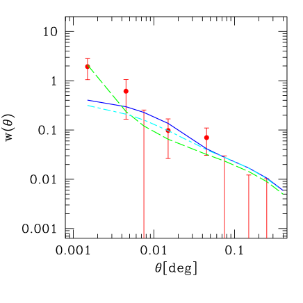
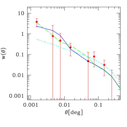
Figure 5: Angular correlation function $w(\theta)$ for the low-z (left-hand panel), and high-z (right-hand panel) samples. The solid (blue) curves represent the best HON fits to the data obtained under the assumption that the distribution of galaxies within their dark matter haloes mirrors that of the dark matter (chosen to be described by a NFW profile, cfr. Section 4), while the dashed (green) curves are the best fits obtained for a steeper galaxy profile, $\rho\propto r^{-3}$. The long-short dashed (cyan) curves correspond to the best 1-parameter fits obtained by setting in eq. (5) $\alpha=0$ and $N_{0}=1$. The negative $w(\theta)$ data-points in the $\chi^{2}$ analysis of the low-z sample have been treated as in §3.1 (see text for details).

In more operative terms, we have calculated $\xi^{1h}$ and $\xi^{2h}$ using the Sheth & Tormen (1999) prescriptions for the halo mass function and the large-scale bias, while the mass auto-correlation function was computed by following a revised version of the method of Peacock & Dodds (1996) which takes into account the spatial exclusion between haloes (i.e. two haloes cannot occupy the same volume). As a starting working hypothesis, the radial profile of the galaxy distribution within their halos is assumed to follow that of the dark matter for which we adopt a NFW profile (Navarro, Frenk & White, 1997). Finally, we allowed the parameters in eq. (8) to vary within the following ranges:
$0\leq\alpha\leq 2$; $10^{11}\leq M_{{\rm min}}/M_{\odot}\leq 10^{14}$; $-3\leq\log_{10}(N_{0})\leq 0$.

Values for these three parameters have been then determined through a minimum $\chi^{2}$ technique by simultaneously fitting the observed $w(\theta)$ (where for the low-z sample we have treated the negative $w(\theta)$ values as in §3.1) and the estimated number density $\bar{n}_{G}$ of sources in both the low-z and high-z samples (cfr. Table 2). The angular correlation function was computed from eq. (2), with $\xi$ obtained as explained above and the redshift distributions shown in Figure  1. The best-fit parameters for the HON of both the low-z and high-z sample are summarized in Table 2; the quoted errors correspond to $\Delta\chi^{2}=1$. The uncertainties associated with $\alpha$ and especially to $M_{\rm min}$ are much smaller than those corresponding to the normalization parameter $N_{0}$ as while the first two quantities are constrained by both the large-scale and small-scale behaviour of $\xi$, according to our model $N_{0}$ only enters the description of the spatial two-point correlation function in the sub-halo regime (cfr. eqs 13 and 14 of Porciani et al. 2004).

The theoretical angular correlation functions corresponding to the best-fit HON parameters for both the low-z and high-z sample are represented by the solid (blue) curves in Figure 5. Since the high-z sample includes a fraction of sources without estimated redshifts, we have also re-run the HON method by only including in the calculation of the comoving number density $\bar{n}_{G}$ sources with assigned photo-z. The results are virtually identical to those reported in Table 2.

As it is possible to notice from Figure 5, the HON does a good job at reproducing the observed $w(\theta)$ at intermediate-to-large angular scales both in the case of the low-z sample and for the high-z sample. However, as it is particularly evident in the low-z plot, it cannot successfully describe the steep rise of the measured two-point correlation function below $\sim 0.005$ degrees. The reason is quite easy to understand: strong contributions to the 1-halo correlation function $\xi^{1h}$ (i.e. the portion of $\xi$ which determines its behaviour on scales smaller than the virial radius) are mainly due to high values of $\alpha$ and $N_{0}$. The magnitude of $\alpha$, together with that of $M_{\rm min}$, is however also determined by the large-scale behaviour of $w(\theta)$. Furthermore, all three quantities enter the calculation of the predicted number density $\bar{n}$ via equation (4) and the number of possible values and combinations is strictly ruled by the requirement that the predicted $\bar{n}$ matches (within 2$\sigma$ in our case) the observed, $\bar{n}_{G}$, one. It follows that the best-fit curves plotted in Figures 5a and 5b below $\theta\sim 0.03^{\circ}$ in the low-z case and $\theta\sim 0.01^{\circ}$ for the high-z sample represent the largest possible small-scale contributions to the observed $w(\theta)$ subject to the constraints put by the large-scale behaviour of $w(\theta)$ and by the observed number density of the sources that produce the clustering signal. Furthermore, we note that large values for $\alpha$ and $N_{0}$, as well as more extreme choices for the second moment $\sigma(M)$ of the galaxy distribution in (5), would only determine a boost of $w(\theta$) on the smallest angular scales probed by our analysis (i.e. an approximately vertical shift of the projected contribution of $\xi^{1h}$), but cannot radically change its shape, which shows a smooth rise followed by a plateau in net contrast with the steep jump of the observed data points on scales smaller than at least $\theta\sim 0.003$ degrees. The model as it is cannot do any better than this.

The most likely solution to this ’small-scale crisis’ comes from releasing the assumption that the distribution of galaxies within their halos follows that of the dark matter. This working hypothesis was used both for simplicity and also because locally the halo distribution of both late-type and early-type galaxies can be nicely described by a NFW profile (see e.g. Magliocchetti & Porciani 2003). However, this does not have to be necessarily true at high redshifts. As an alternative approach, we have then considered the possibility for the galaxies to be more concentrated than the underlying dark matter, and in order to reproduce this effect we have taken a galaxy density profile of the kind $\rho\propto r^{-3}$ (hereafter called PL3; see Magliocchetti & Porciani 2003).

The best fitting curves obtained within the HON framework in the PL3 case are shown in Figures 5a and 5b by the dashed (green) curves. The corresponding best-fitting values for $M_{\rm min}$, $\alpha$ and $N_{0}$ are given in Table 2. As expected, a model which now foresees a steep profile for the galaxy distribution can provide an excellent fit to the observed small-scale rise of $w(\theta)$ in both the low-z and high-z sample. Furthermore, the best fitting values for the HON in the PL3 case are almost identical to those obtained by considering NFW profiles. This shows that the average behaviour for the spatial distribution of galaxies within their dark matter halos can be recovered from investigations of the small-scale features of the angular/spatial two-point correlation function in a ’clean’ way as such features can be modelled independently of the other parameters adopted to describe the clustering properties of a given astrophysical population.

So, which kind of information can we infer from this small-scale behaviour of $w(\theta)$? Locally, Magliocchetti & Porciani (2003) find that galaxy distributions of the PL3 kind are strongly rejected by the data, as small-scale measurements of the two-point correlation function prefer smoother profiles such as NFW or $\rho\propto r^{-2.5}$. However, at very low redshifts it is reasonable to expect the majority of dark matter halos to be virialized and therefore be to reasonably described (at least beyond the very small scales, see e.g. Bukert 1995) by NFW-like profiles. Two options are instead possible at such high redshifts. The first one is that galaxies still do trace the underlying distribution of the dark matter within their halos, and it is the dark matter itself which does not follow NFW-like profiles. The second option is instead that galaxies are simply more radially concentrated than the dominant dark matter counterpart. Whatever the favourite choice, one thing is clear. On sub-halo scales, 24$\mu$m-selected galaxies at redshifts $z\mathrel{\hbox to0.0pt{\lower 3.0pt\hbox{$\sim$}\hss}\raise 2.0pt\hbox{$>$}}0.6$ are more strongly radially concentrated than their low-redshift counterparts. Such a strong concentration is indicative of a strong interaction between galaxies which reside in the proximity of the halo centres, and we expect such a strong interaction to eventually drive a substantial number of mergers. It is possibly not a random coincidence that bright 24$\mu$m-selected sources at intermediate-to-high redshifts are in general associated to very intense star-forming systems; the excess of proximity between such galaxies would eventually lead to gas-rich mergers which could easily trigger enhanced star-formation activity like the ones observed. In passing, we note that evidence for an upturn (although less significative than ours) on scales $r\mathrel{\hbox to0.0pt{\lower 3.0pt\hbox{$\sim$}\hss}\raise 2.0pt\hbox{$<$}}0.2/h$ Mpc has also been recently reported by Gilli et al. (2007) for their sample of $z\sim 1$, 24$\mu$m-selected sources in the GOODS fields.

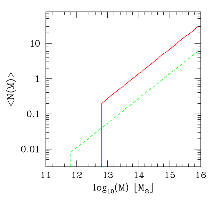
Figure 6: Average number of galaxies $\langle N\rangle$ per dark matter halo of specified mass $M$ (expressed in $M_{\odot}$ units). The solid (red) line represents the case for the high-z sample, while the dashed (green) line is for the low-z sample.

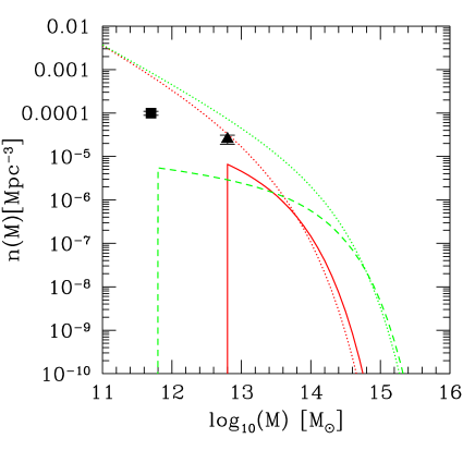
Figure 7: Number of galaxies per unit of (log) dark matter mass and volume as evaluated following eq.(4) for the best fitting values of the HON presented in Figure 6 at the effective redshifts $z\sim 0.8$ and $z\sim 2$ of the two datasets under exam. The solid (red) line represents the result for the high-z sample, while the dashed (green) line is for low-z sample. For comparison, the two dotted lines indicate the Sheth & Tormen (1999) mass function $n(M)$ of dark matter haloes (the higher/green curve corresponding to the low-z sample). The filled triangle indicates the observed number density of sources in the high-z sample, while the filled square is for the low-z sample.

The best average number of galaxies $\langle N\rangle$ as a function of halo mass for the two analysed samples (and in the PL3 case) are presented in Figure 6 (solid/red line for the high-z sample), while the galaxy mass function as coming from eq. (4) for the best-fit values of the HON for the high-z sample (solid/red curve) and in the case of the low-z sample (dashed/green curve) are illustrated by Figure 7. Despite the large uncertainties due to the relatively poor statistics, a number of interesting features can be gathered from these plots. Sources belonging to the high-z sample appear to be exclusively located in very massive, $M\mathrel{\hbox to0.0pt{\lower 3.0pt\hbox{$\sim$}\hss}\raise 2.0pt\hbox{$>$}}10^{13}M_{\odot}$, structures, identifiable with groups-to-clusters of galaxies. These galaxies are quite common within their halos ($\langle N\rangle$ between $\sim 0.6$ and $\sim 0.06$ at the lowest possible masses where the sources start appearing), and we note that since $\langle N\rangle$ is a quantity which is averaged all over the dark matter halos more massive than $M_{\rm min}$, in the most extreme case our results imply that more than one in two of all the structures with masses $M\sim 10^{13}M_{\odot}$ host a high-z, $F_{24\mu\rm m}\geq 400\mu$Jy galaxy. Furthermore, their number sensibly increases with the richness of the structure which hosts them. At around $M\sim 10^{15}M_{\odot}$, their average abundance is between 5 and 20 sources per halo ($\sim 10$ for the best-fit model), value which is not in disagreement with the typical figures for the number of bright, $L>L^{*}$ galaxies associated to local rich clusters (e.g. Terlevich, Caldwell & Bower, 2001).

On the other hand, the low-z sample seems to be made of galaxies of much smaller mass ($M_{\rm min}\simeq 10^{12}M_{\odot}$). Also, these objects are very rare (in the most unfavourable case we get $\langle N\rangle\sim 10^{-3}$ at the lowest possible masses at which the sources start appearing, i.e. only 0.1% of the ’allowed’ halos host a galaxy of the kind which make the low-z sample), even though their number – as it was the case for the high-z sample – sensibly increases with halo mass; this determines an overall flatness of the galaxy mass function at least up to $\sim 10^{14}M_{\odot}$.

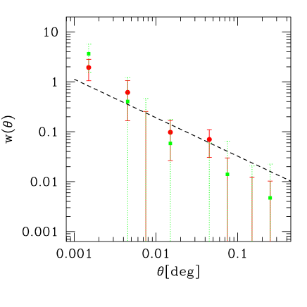
Figure 8: Angular two-point correlation function $w(\theta)$ for low-z UDS-SWIRE sources brighter than 0.5 mJy (210 objects; green squares and associated, dotted, errorbars) as compared to that presented in §3.1 (red circles). The dashed line represents the best-fit to the low-z, $F_{24\mu\rm m}\geq 0.4$ mJy, sample obtained as in §3.1

From the analyses performed in Sections 3 and 4 it appears clear that the populations probed by the high-z and low-z samples are very different from each other. One might argue that the higher clustering level reported at redshifts $z\mathrel{\hbox to0.0pt{\lower 3.0pt\hbox{$\sim$}\hss}\raise 2.0pt\hbox{$>$}}1.6$ can be simply attributed to the fact that since we are dealing with a flux-limited survey rather than a volume-limited one, higher redshifts probe more intrinsically luminous sources which are in general hosted by more massive halos and therefore result more strongly clustered. However, we note that this cannot be the only explanation for such a strong difference between the clustering properties of the low-z and the high-z sample. Sources in the high-z sample are in fact so strongly clustered that it would only take a small fraction of them in the low-z sample (say of the order of 20%) to sensibly boost the low-z clustering signal. This does not seem to happen. Obviously, the ultimate evidence for a strong evolution of the clustering signal of 24$\mu$m-selected sources between $z\sim 2$ and $z\sim 1$ could in principle only be obtained by comparing volume-limited rather than flux-limited samples. Given the Spectral Energy Distributions of these sources, this would imply including in our analysis only objects brighter than $\sim 1$ mJy in the low-z sample. Unfortunately, the number of such low-z sources is very limited and insufficient to allow for a statistically significant estimate of $w(\theta)$. However, as a sensible alternative we can consider a sub-sample of low-z sources brighter than the chosen 0.4 mJy limit, which contains enough objects to provide meaningful results for the two-point correlation function. We have then decided to restrict our analysis to low-z galaxies brighter than $F_{24\mu\rm m}=0.5$ mJy. We note that, despite the marginal flux increment, this new sample only contains 210 sources, i.e. almost a factor 2 less than the original, $F_{24\mu\rm m}\geq 0.4$ mJy, dataset. The corresponding $w(\theta)$ is shown by the (green) squares in Figure 8.
Under the assumption of no cosmological evolution for those 24$\mu$m-selected galaxies residing at $z\sim 2$ and taking into account the different volumes occupied by the two low-z and high-z samples, we would expect $\sim 80$ very massive sources in the $0.6\leq z\leq 1.2$ redshift interval. And if these sources indeed existed at $z\sim 1$, they would constitute $\sim 40$% of the $F_{24\mu\rm m}\geq 0.5$ mJy low-z sample, to be compared to $\sim 25$% of the $F_{24\mu\rm m}\geq 0.4$ mJy one. This sensible increase in the relative weight of very massive sources (which now would make only slightly less than 50% of the entire low-z dataset) in the $z\sim 1$ sample is expected to determine a sensible boost of the correlation function signal. But this is does not happen, as the observed clustering amplitude of $F_{24\mu\rm m}\geq 0.5$ mJy objects is virtually identical to that obtained in §3.1 (and reproduced in Figure 8 by the red circles for sake of clarity) for a lower flux cut.

Massive galaxies undergoing intense activity such as star-formation or AGN accretion seem to disappear when going from redshifts $\sim 2$ to $\sim 1$. At this lower redshifts, obscured star forming and AGN activity seem to be segregated in much lower-mass systems. Obviously, the present data cannot say anything on the eventual presence of active low-mass galaxies at redshift $\sim 2$, but they tend to strongly exclude the presence of intense activity from very massive systems below redshifts - say - 1.5.

4.1 The Halo Bias Approach

One might wonder about the need of using somewhat sophisticated tools such as the Halo Occupation formalism in the case of datasets characterized by a low signal-to-noise ratio as the ones we are dealing with. To answer this question, we have considered the more standard halo bias approach (Mo & White 1996) which describes the clustering signal of a chosen population of extragalactic sources as the product between the two-point correlation function of the dark matter and the square of the so-called bias function, a quantity which solely depends on the minimum mass $M_{\rm min}$ of the halos in which the astrophysical objects reside. Such an approach assumes a one-to-one correspondence between dark matter halos and hosted sources and can be thought as a special case within the HON framework corresponding in equation (5) to $\alpha=0$, $N_{0}=1$ and $\sigma(M)=0$. Once the cosmology is fixed, this is a 1-parameter model which might seem more appropriate for the description of clustering signals affected by large noise. The angular two-point correlation functions $w(\theta)$ predicted by the halo bias model for the low-z and high-z samples have then been computed once again by following eq.(2) and the best values for $M_{\rm min}$ in the two cases have been found by a $\chi^{2}$-fit to the observed clustering signal. We find ${\rm Log}M_{\rm min}=13.3^{+0.2}_{-0.4}$ and ${\rm Log}M_{\rm min}=12.4^{+0.4}_{-0.6}$ respectively for the high-z and low-z sample, and the corresponding $w(\theta)$’s are represented in Figures 5a and 5b by the (cyan) long-short dashed curves. These values are in good agreement with those obtained by using the full HON approach presented earlier in this Section, the somewhat higher figures found for $M_{\rm min}$ in this latter case being simply due to the fact that $\alpha$ and $M_{\rm min}$ are covariant quantities, so that within the HON framework higher $\alpha$ in general correspond to lower $M_{\rm min}$. This provides reassuring evidence for the goodness of the results derived from the HON analysis.

On the other hand, the 1-parameter halo bias model suffers from a number of problems which can instead be overcome by using the full HON approach. The first problem is encountered once the values of $M_{\rm min}$ as obtained above are plugged in the calculation of the number density of sources via eq. (4). In the high-z case, the figure we obtain ($\bar{n}\sim 1.5\cdot 10^{-5}$ Mpc^-3) is in good agreement with the observational findings presented in §2. However, for the low-z sample we find $\bar{n}\sim 8.5\cdot 10^{-3}$ Mpc^-3, value which is about 10 times larger that what observationally determined. This big discrepancy stems from the erroneous a priori assumption of the 1-parameter halo bias model for a one-to-one correspondence between dark matter halos and astrophysical sources. As shown by the results of the full HON analysis (cfr. Table 2), such a working hypothesis could hold for the high-z sample which presents $N_{0}$ values not too far from unity, but badly fails when one deals with rare sources such a those characterizing the low-z sample. The HON approach instead provides a self-consistent answer for both the clustering properties and the number density of $z\sim 1$ sources.

A second problem related to 1-parameter models such as the halo bias is that, by merely concentrating on the clustering properties of the dark matter halos, they are unable to describe the clustering behaviour of astrophysical sources on sub-halo scales. This feature is evident in Figures 5a and 5b. Although reproducing the large-scale trend of the observed $w(\theta)$’s on large scales, the halo bias model systematically underestimates the observed clustering signal at small angular distances. The problem is particularly bad at the smallest angular scales probed by our analysis whereby, in the case of $z\sim 2$ sources, this model predicts $\sim 3$ pairs to be compared to the 9 (or 10, see §2) observed in our dataset. For the lower redshift sample the predicted figure is again $\sim 3$, while the number of observed pairs is 11. The full HON approach instead works much better at describing the clustering properties of extragalactic sources at all scales and can provide a correct match between observed and predicted quantities even at the shortest distances (the number of predicted pairs at $\theta\sim 0.0015$ degrees within the HON framework is $\sim 5$ and $\sim 9$ respectively for a NFW and a PL3 model at $z\sim 2$ and $\sim 4$ and $\sim 11$ at $z\sim 1$). We note, for comparison, that the ’$\gamma$ model’ exploited in §3, gives $N_{\it low-z}\sim 6$ and $N_{\it high-z}\sim 5$.

5 Conclusions

We have investigated the clustering properties of 24$\mu$m-selected galaxies brighter than 400$\mu$Jy, drawn from the SWIRE and UKIDSS Ultra Deep Surveys. With the help of photometric redshift determinations, we have concentrated on two datasets which include galaxies respectively in the $z=[0.6-1.2]$ (low-z sample) and $z\mathrel{\hbox to0.0pt{\lower 3.0pt\hbox{$\sim$}\hss}\raise 2.0pt\hbox{$>$}}1.6$ (high-z sample) redshift ranges. The low-z sample is made of 350 galaxies, while the high-z sample includes both 182 galaxies with estimated photo-z’s and another 28 sources which do not have any optical or near-IR counterpart. Diagnostics based on the ratio between 8$\mu$m and 24$\mu$m fluxes indicate that these two samples are likely made by a very similar mixture of active star-forming galaxies ($\sim 65$ per cent) and AGN (the remaining $\sim 35$ per cent).

Results obtained by fitting with a power-law of fixed slope $\gamma=1.8$ the observed angular two-point correlation function $w(\theta)$ report an amplitude $A^{hz}=0.010\pm 0.0035$ and $A^{lz}=0.0055^{+0.0015}_{-0.0020}$ ($w(\theta)=A\;\theta^{1-\gamma}$) respectively for the high-z and low-z samples. In more physical coordinates, the above results imply (comoving) correlation lengths for the spatial two-point correlation function $\xi$ (modelled as $\xi=(r/r_{0})^{-\gamma}$) $r_{0}^{hz}=15.9^{+2.9}_{-3.4}$ Mpc and $r_{0}^{lz}=8.5^{+1.5}_{-1.8}$ Mpc, showing that the galaxies in the high-z sample are more strongly clustered that those found at lower redshifts.

A deeper insight on the above findings is provided by the so-called Halo Occupation Scenario which connects the clustering properties of a chosen population of astrophysical objects with some of their physical properties. The key quantity for this kind of analysis is the Halo Occupation Number (HON), i.e. the average number of galaxies enclosed in a halo of given mass $M$, which can be parametrized as $\langle N\rangle=N_{0}\left(M/M_{\rm min}\right)^{\alpha}$, with $M_{\rm min}$ minimum mass for a halo to host one of such galaxies and $N_{0}$ normalization factor which provides information on how common the galaxies under examination are.

At first we have adopted as a working hypothesis that Spitzer-selected galaxies were spatially distributed within their dark matter halos according to the dark matter (NFW) distribution. However, we find that such a model fails at reproducing the high amplitude of the observed $w(\theta$) signal on angular scales $\mathrel{\hbox to0.0pt{\lower 3.0pt\hbox{$\sim$}\hss}\raise 2.0pt\hbox{$<$}}0.003$ degrees both in the low-z and high-z sample. A much better agreement with the data is obtained when we take the galaxies to be very concentrated towards their halo centres, e.g. by assuming a distribution of the kind $\rho\propto r^{-3}$. Such a high concentration – not observed in local data (Magliocchetti & Porciani 2003) – is suggestive of a strong interaction and close encounters between galaxies which reside in the proximity of the halo centres, and we expect such a strong interaction to eventually drive a substantial number of gas-rich mergers which could easily trigger the observed enhanced star-formation activity.

Investigations of the best-fit values for the HON report values ${\rm Log}\left(M_{\rm min}^{hz}/M_{\odot}\right)=12.8^{+0.2}_{-0.4}$; ${\rm Log}N_{0}^{hz}=-0.7^{+0.5}_{-0.5}$; $\alpha^{hz}=0.7^{+0.3}_{-0.5}$ for the high-z sample and ${\rm Log}\left(M_{\rm min}^{lz}/M_{\odot}\right)=11.8^{+0.8}_{-0.8}$; ${\rm Log}N_{0}^{lz}=-2.1^{+1.1}_{-0.9}$; $\alpha^{lz}=0.7^{+0.1}_{-0.3}$ in the case of low-z sources. The above figures indicate that galaxies belonging to the high-z sample are exclusively associated with very massive, $M\mathrel{\hbox to0.0pt{\lower 3.0pt\hbox{$\sim$}\hss}\raise 2.0pt\hbox{$>$}}10^{12.8}M_{\odot}$, structures, identifiable with groups-to-clusters of galaxies. Furthermore, these galaxies are quite common within their halos (in the most extreme case, our results imply that more than one in two of all the structures with masses $M\simeq M_{\rm min}$ host a $z\sim 2$, $F_{24\mu\rm m}\geq 400\mu$Jy galaxy), and their number sensibly increases with the richness of the structure which hosts them. On the other hand, the low-z sample seems to be made of galaxies of much smaller mass ($M_{\rm min}\simeq 10^{11.8}M_{\odot}$). These objects are also very rare; in the most unfavourable case we get that only 0.1% of the ’allowed’ halos host a galaxy of the kind which make the low-z sample.

Such a remarkable difference in the clustering and environmental properties of active sources as seen at $z\sim 2$ and $z\sim 1$ can be hardly attributed to the fact that high redshift galaxies are intrinsically brighter than their lower redshift counterparts (cfr. §4). Indeed, despite the large uncertainties determined by the poor statistics of the considered datasets, our results indicate that the populations probed by the high-z and low-z samples are very different from each other: massive active galaxies seem to disappear when going from $z\sim 2$ to $z\sim 1$, and at this lower redshifts all the AGN and starforming activity appears to be segregated in much lower-mass systems (see also the results of Gilli et al. 2007 who find for their bright, $z\sim 0.7$, 24$\mu$m-selected galaxies in the GOODS fields a correlation length $r_{0}\sim 8$ Mpc.). We stress that, while investigations of the luminosity function of 8$\mu$m-rest frame-selected sources have already established a strong luminosity evolution of sources between redshifts $\sim 2$ and $\sim 1$ (e.g. Caputi et al. 2007), clustering measurements provide a unique tool to determine the physical nature of such an evolution. Our work can in fact show that the strong differential evolution of the 24$\mu$m LF is not simply due to the fact that the less luminous sources at $z\sim 1$ are dimmed versions of the galaxies at higher-z (i.e. pseudo-passive evolution), but indeed has to be attributed to different populations of objects inhabiting different dark matter haloes and structures.

The general picture which then emerges from the results of this paper points to a differential evolution for high-mass and low-mass systems. Massive systems form early in time at the rare peaks of the density field. Their intense activity, both in terms of star-formation and AGN accretion, is strongly favoured (if not triggered) by numerous close encounters and gas-rich mergers happening in the proximity of the centres of the massive/cluster-like structures in which these sources reside. Such an active phase is relatively short-lasted and already below $z\sim 1.5$ these objects evolve as optically passive galaxies, in most of the cases ending up as the supermassive galaxies which locally reside in cluster centres and which show a remarkable tendency for enhanced radio activity (see e.g. Best et al. 2006; Magliocchetti & Brüggen 2007). Lower ($M\mathrel{\hbox to0.0pt{\lower 3.0pt\hbox{$\sim$}\hss}\raise 2.0pt\hbox{$<$}}10^{12}M_{\odot}$) mass systems are instead characterized by an active phase which lasts down to lower redshifts. Also in this case, the AGN and star forming activities seem to be favoured by the strong concentration of these sources towards their halo centres. These objects will eventually end up as ’typical’ early-type galaxies which favour relatively (but not extremely) dense environments.

At present, studies on the evolutionary properties of dust-enshrouded active systems like those we have investigated in this work are hampered by the lack of surveys which can probe their peak of emissivity to low enough fluxes and also by the extreme difficulty of getting spectroscopic redshifts for such optically faint sources. The forthcoming advent of instruments such as Herschel, SCUBA-2 and ALMA will finally fill in this gap and provide the community with ’the ultimate truth’ on most of the issues connected with galaxy formation and evolution.

References

- [Baugh2005] Baugh C.M., Lacey C.G. Frenk C.S., Granato G.L., Silva L., Bressan A., Benson A.J., Cole S., 2005, MNRAS, 356, 1191
- [1] Bolzonella M., Miralles J.-M., & Pelló, R., 2000, A&A, 363, 476
- [Berletal2003] Berlind A.A. et al., 2003, ApJ, 593, 1
- [Best2007] Best P.N., von der Linden A., Kauffmann G., Heckman T. M., Kaiser C. R., 2006, astro-ph/0611197
- [Brand2006] Brand K., et al., 2006, ApJ, 644, 143
- [2] Bruzual G., Charlot S., 2003, MNRAS, 344, 1000
- [Buk1995] Bukert A., 1995, ApJ, 447, L25
- [Bundi2005] Bundy K., et al., 2006, ApJ, 651, 120
- [cap2007] Caputi K.I., et al., 2007, astro-ph/0701283
- [chap2005] Chapman S.C., Blain A.W., Smail I., Ivison R.J., 2005, ApJ, 622, 772
- [cimatti2004] Cimatti A., et al., 2004, Nature, 430, 184
- [3] Cirasuolo et al. 2007, MNRAS submitted, astro-ph/0609287
- [4] Coleman, G.D., Wu, C.-C., Weedman, D.W., 1980, ApJS, 43, 393
- [coppin2006] Coppin K., et al., 2006, MNRAS, 372, 1621
- [cowie1996] Cowie L.L., Songaila A., Hu E., Cohen J.G., 1996, AJ, 112, 839
- [Eales2000] Eales S., Lilly. S., Webb T., Dunne L., Gear W., Clements D., Yun M., 2000, AJ, 120, 2244
- [\citeauthoryearEllis et al.1997] Ellis R.S., Smail I., Dressler A., Couch W.J., Oemler A.J., Butcher H., Sharples R.M., 1997, ApJ, 483, 582
- [Fadda2006] Fadda D. et al., 2006, AJ, 131, 2859
- [fang2004] Fang F., et al., 2004, ApJS, 154, 35
- [far12006] Farrah D., et al., 2006a, ApJ, 641, L17
- [far22006] Farrah D., et al., 2006b, ApJ,643, L139
- [\citeauthoryearFontana et al.2004] Fontana A., et al., 2004, A&A, 424, 23
- [fouc2007] Foucaud S. el al., 2007, MNRAS, 376, L20
- [\citeauthoryearGilli et al.2007] illi R. et al. 2007, to appear on A&A, arXiv:0708.2796
- [\citeauthoryearGlazebrook et al.2004] Glazebrook K., et al., 2004, Nature, 430, 181
- [gra2004] Granato G.L., De Zotti G., Silva L., Bressan A., Danese L., 2004, ApJ, 600, 580
- [graz2006] Grazian A. et al., 2006, A&A, 453, 507
- [guzzo2000] Guzzo L. et al., 2000, ASPC, 200, 349
- [Hamilton1993] Hamilton A.J.S., 1993, ApJ, 417,19
- [Hatton2003] Hatton S., Devriendt J.E.G., Ninin S., Bouchet F.R., Guiderdoni B., Vibert D., 2003, MNRAS, 343, 75
- [Heavens2004] Heavens A., Panter B., Jimenez R., Dunlop J., 2004, Nature, 428, 625
- [\citeauthoryearHolden et al.2005] Holden B.P., et al., 2005, ApJ, 626, 809
- [Houck2005] Houck J.R., et al., 2005, ApJ, 622, L105
- [Hughes1998] Hughes D.H., et al., 1998, Nature, 394, 241
- [Houg2006] Houges D., et al, 2006, AAS, 209 8307
- [5] Kinney, A.L., Calzetti, D., Bohlin, R. C., McQuade, K., Storchi-Bergmann, T., Schmitt, H.R., 1996, ApJ, 467, 38
- [Knudsen2006] Knudsen K.K., et al., 2006, MNRAS, 368, 487
- [Kri2007] Kriek M., et al., 2007, astro-ph/0611724
- [6] Lawrence, A., et al. 2006, MNRAS submitted, astro-ph/0604426
- [7] Le Fevre O. et al., 2005, A&A, 439, 877
- [8] Lonsdale C.J., et al. 2003, PASP, 115, 897
- [9] Lonsdale C.J., et al. 2004, ApJS, 154, 54
- [Mad2003] Madgwick D. et al., 2003, MNRAS, 344, 847.
- [Maglio1999] Magliocchetti M., Maddox S.J., 1999, MNRAS, 306, 988
- [Maglio12003] Magliocchetti M., Porciani C., 2003, MNRAS, 346, 186
- [Maglio12007] Magliocchetti M., Silva L., Lapi A., De Zotti G., Granato G.L., Fadda D., Danese L., 2007, MNRAS, 375, 1121
- [Maglio22007] Magliocchetti M., Brüggen M., 2007, to appear in MNRAS, arXiv:0705.0574
- [Mc2006] McLure R.J., et al., 2006, MNRAS, 372, 357
- [10] Mignoli, M., et al., 2005, A&A, 437, 883
- [Mo1996] Mo H.J., White S.D.M., 1996, MNRAS, 282, 347
- [\citeauthoryearNaab, Khochfar, & Burkert2006] Naab T., Khochfar S., Burkert A., 2006, ApJ, 636, L81
- [NFW1997] Navarro J.F., Frenk C.S., White S.D.M., 1997, ApJ, 490, 493
- [Norberg2002] Norberg P. et al., 2002, MNRAS, 332, 827
- [Peacock 1996] Peacock J.A., Dodds S.J., 1996, MNRAS, 267, 1020
- [Peebles1980] Peebles P.J.E., 1980, The Large-Scale Structure of the Universe, Princeton University Press
- [Porci1 2004] Porciani C., Magliocchetti M., Norberg P., 2004, MNRAS, 355, 1010
- [Pozzi2007] Pozzi F., et al, 2007, arXiv:0704.0735
- [\citeauthoryearSaracco et al.2006] Saracco P., et al., 2006, MNRAS, 367, 349
- [Scott2002] Scott S.E., et al., 2002, MNRAS, 331, 817
- [11] Sekiguki K., et al., 2005, in Renzini A. & Bender R., ed., Multiwavelength mapping of galaxy formation and evolution. Springer-Verlag, Berlin, p82
- [sheth1 2001] Sheth R.K., Diaferio A., 2001, MNRAS, 322, 901
- [sheth 1999] Sheth R.K., Tormen G., 1999, MNRAS, 308, 119
- [sper 2003] Spergel D.N. et al., 2003, ApJS, 148, 175
- [12] Surace J., et al. 2005, Technical report, The SWIRE Data release 2, http://swire.ipac.caltech.edu/swire/astronomers.html
- [ter 2001] Terlevich A.I., Caldwell N., Bower, R. G., 2001, MNRAS, 326, 1547
- [treu2005] Treu T., Ellis R.S., Liao T.X., van Dokkum P.G., 2005, ApJ, 622, L5
- [van Dokkum 2005] van Dokkum P.G., 2005, AJ, 130, 2647
- [Yan2005] Yan L., et al., 2005, ApJ, 628, 604
- [Yan12007] Yan L., et al., 2007, ApJ, 658,778
- [13] Warren S.J., et al. 2007, MNRAS, 375, 213
- [Willum1997] Willumsen J.V., Freudling W, Da Costa L.N., 1997, ApJ, 481, 571.
- [Zehavi2005] Zehavi I. et al., 2005, ApJ, 630,1