Unveiling dark halos in lensing galaxies

Abstract

We present a spatially resolved comparison of the stellar-mass and total-mass surface distributions of nine early-type galaxies. The galaxies are a subset of the Sloan Lens ACS survey (or SLACS; Bolton et al., 2006). The total-mass distributions are obtained by exploring pixelated mass models that reproduce the lensed images. The stellar-mass distributions are derived from population-synthesis models fit to the photometry of the lensing galaxies. Uncertainties – mainly model degeneracies – are also computed. Stars can account for all the mass in the inner regions. A Salpeter IMF actually gives too much stellar mass in the inner regions and hence appears ruled out. Dark matter becomes significant by the half-light radius and becomes increasingly dominant at larger radii. The stellar and dark components are closely aligned, but the actual ellipticities are not correlated. Finally, we attempt to intuitively summarize the results by rendering the density, stellar-vs-dark ratio, and uncertainties as false-colour maps.

1 Introduction

In the current paradigm of galaxy formation, the building block of structure is a dark matter halo, consisting mainly of non-baryonic dark matter together with $\sim 15\%$ baryons in the form of gas. Dark halos are thought to originate from the collapse of primordial density fluctuations, growing unimpeded until virial equilibrium is reached. Within these halos the baryonic component dissipates energy, collapsing further towards the center and eventually forming the visible galaxy. Subsequent mergers redistribute the matter within halos.

To work out the details of the basic picture, which goes back to White & Rees (1978), it is essential to determine the connection between the visible galaxies and dark halos. Strong gravitational lensing by galaxies is potentially a very useful way of doing this, since the total mass of a lensing galaxy is relatively easy to constrain. Also, since lensing tends to be more effective for distant galaxies ($z_{\rm lens}\sim 0.1$ to 1), it nicely complements the stellar-dynamical techniques applicable in nearby galaxies.

The difficulty with lensing galaxies (that is to say, galaxies producing multiple images of background sources) is that they are relatively rare. Till recently, only about 80 were known. But recently, 28 new galaxy lenses have been discovered by the Sloan Lens ACS Survey (SLACS; Bolton et al., 2006) thanks to a new survey strategy, which eventually may double the number of strong lenses. The method is to select galaxies from the Sloan survey (York et al., 2000) that have emission lines indicating high-redshift background objects, and then to image these candidates using the Advanced Camera for Surveys on the Hubble Space Telescope.

A basic analysis of a sample of galaxy lenses is to fit simple lens models and then compute $M/L$ and its evolution with redshift. This was first done by Keeton et al. (1998). An extension is to place lensing galaxies on the Fundamental Plane of ellipticals, using a measured or model-derived velocity dispersion (Kochanek et al., 2000; Rusin et al., 2003; Treu et al., 2006). Other work (Treu & Koopmans, 2004; Koopmans et al., 2006) compares lens models with the measured dispersions to constrain the mass profiles of the galaxies. These studies have found no unexpected features or trends with redshift, and argue in favor of passive evolution.

A more detailed analysis involves modeling both the lens mass distribution and the stellar population. The star-formation history is not well-constrained by the observed fluxes and colours and must be marginalized over, but the stellar mass is fairly insensitive to model assumptions apart from the initial mass function (IMF). The lensing mass distribution, when aggressively modeled, turns out to have much larger uncertainties than simple models assume; nevertheless, the uncertainties can be estimated and useful conclusions drawn. Ferreras et al. (2005) found massive ellipticals to show a transition from no significant dark matter within $R_{e}$ to dark-matter dominance by $5R_{e}$, whereas lower-mass galaxies showed no significant dark halos even at $5R_{e}$. The radial gradient in the dark-matter fraction agreed with the results on nearby galaxies derived from stellar dynamics (Napolitano et al., 2005).

In this paper we extend the detailed comparison of stellar and total mass to two dimensions, using a subsample of the SLACS lenses. All the SLACS objects have a background galaxy that is lensed into two or four extended images. In nine of the objects, we can identify small features within the extended images. For lenses showing point-like multiply-imaged features there is a well-developed technique for reconstructing the projected mass distribution, along with uncertainty estimates (Saha & Williams, 2004). Accordingly we take these nine lenses as our sample. The stellar mass content is estimated by combining the available photometry of the lensing galaxies with population-synthesis models (Bruzual & Charlot, 2003).

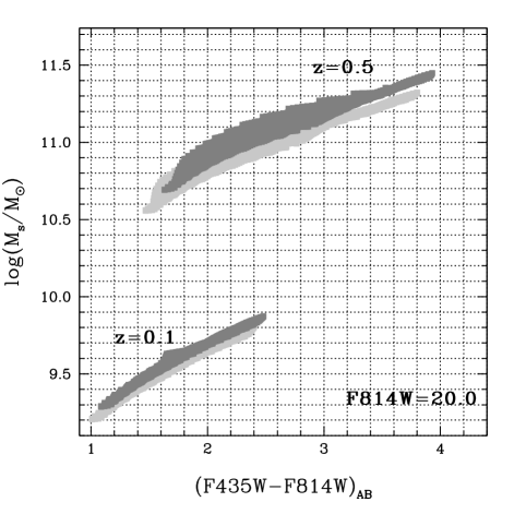
Figure 1: Stellar masses derived from the available photometry. The predictions of the Bruzual & Charlot (2003) models are shown for a Chabrier (2003) IMF. A galaxy with apparent magnitude $\rm F814W=20$ is considered at two different redshifts as labelled. The shaded regions span the model predictions when assuming a wide range of $\tau$ models (i.e., an exponentially decaying star formation history at fixed metallicity). The dark/light shaded regions correspond to a formation redshift of $z_{F}=5$ and $2$, respectively, and all span a range of star formation timescales ($-1<\log\tau({\rm Gyr})<+1$) and metallicities ($-1<\log Z/Z_{\odot}<+0.3$).

2 Mapping the total mass

We use the pixelated lens reconstruction method implemented in the PixeLens program. The algorithm is motivated and described in detail in Saha & Williams (2004), but basically it consists of two ideas.

The first idea is to express the lensing data as a set of linear constraint equations on the mass distribution. We assume that the centroids of multiple images are measured with negligible error, which — at HST resolution — is a very good approximation. Then the remaining unknowns are the source position and the lens mass distribution, and both of these enter the lens equation linearly (cf. Equation 5 in Saha & Williams, 1997). The lens is expressed as a superposition of mass tiles or pixels, although a superposition of basis functions is also possible (Trotter et al., 2000). A prior on the lens can be expressed as linear inequalities. Specifically, we require the mass distribution to (i) be non-negative, (ii) be centrally concentrated, with the local density gradient pointing $\leq 45^{\circ}$ away from the center, (iii) be inversion symmetric (i.e. symmetric with respect to rotation by $180^{\circ}$; optional), (iv) have no pixel more than twice the sum of its neighbors, except possibly the central pixel, and (v) the circularly averaged mass profile to be steeper than $R^{-0.5}$, where $R$ is the projected radius. Item (v) is assumed (for galaxies) since stellar dynamics or other methods never give $\rho(r)$ as shallow as $r^{-1.5}$ (e.g., Binney et al., 1991; Gerhard et al., 2001). These various equations and inequalities give an underdetermined linear system analogous to Schwarzschild’s problem in stellar dynamics.

The second idea (suggested by Williams & Saha, 2000) is to sample the mass maps allowed by the data and prior, through a Monte-Carlo method. The result is an ensemble of lens models. Uncertainties on any parameter of the lens can be derived from the model ensemble in the usual way. The ensemble-average will automatically satisfy the data and prior constraints, since they are linear. This makes the ensemble-average model a good choice for representing a single model. For a detailed illustration of the ensemble method, see the Appendix in Saha, Williams & Ferreras (2007).

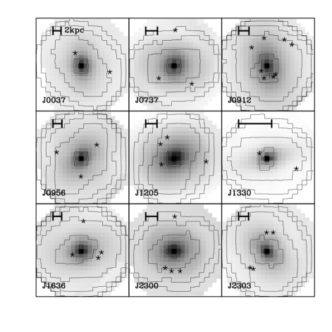
Figure 2: Projected mass maps of the lensing galaxies. The gray scale represents $\Sigma_{\rm stel}$ while the contours show $\Sigma_{\rm tot}$. The latter are in multiplicative steps of $10^{0.4}$ (like a magnitude scale). The star symbols mark multiply-imaged features of the background source. The bar in each panel indicates 2 kpc.

For each lens we computed an ensemble of 200 mass maps of $21\times 21$ pixels each. To derive radial profiles we circularly-averaged the mass maps. This procedure naturally yields ensembles of radial profiles, hence an estimate of the uncertainty.

In the lens models the enclosed mass is best constrained at projected radii similar to the images themselves (roughly speaking, around the Einstein radius), whereas at smaller and larger radii, the enclosed mass becomes progressively more uncertain. This is simply the well-known steepness degeneracy in lensing theory (see e.g., Saha, 2000). As a result, the enclosed mass profile and its error-bars have a characteristic butterfly shape.

To what extent velocity dispersions can break lensing degeneracies remains an open question. Studies using velocity dispersions as constraints on lenses tend to be optimistic. However, stellar-dynamical degeneracies associated with kinematics are also known (Valluri et al., 2004; Cretton & Emsellem, 2004) and it is not clear that these will be orthogonal to lensing degeneracies. Also, current methods for incorporating kinematics into lens models assume spherical symmetry. For these reasons we do not include kinematics in the lens models.

We do not attempt to fit the extended images. Now, a model fitted to point-like images automatically provide a predictions for arcs that would be generated by a conical light profile (i.e. a circularly symmetric model; Saha & Williams (2001)) and these predicted arcs generally do yield a good approximation to observed arcs. Hence disregarding the extended images does not sacrifice as much information as might at first appear. Fitting a better source distribution is a straightforward linear image-reconstruction problem if the lens model is fixed. But using the source structure to improve the lens fit is much harder. Several papers propose schemes that iteratively fit lens and source models. But they either assume a restricted parameterized form for the lens (e.g., Wallington, Narayan & Kochanek, 1994; Dye & Warren, 2005; Brewer & Lewis, 2006; Koopmans et al., 2006) or allow the lens model to be free form (Koopmans, 2005; Suyu & Blandford, 2006) but need it to be close to a starting guess.

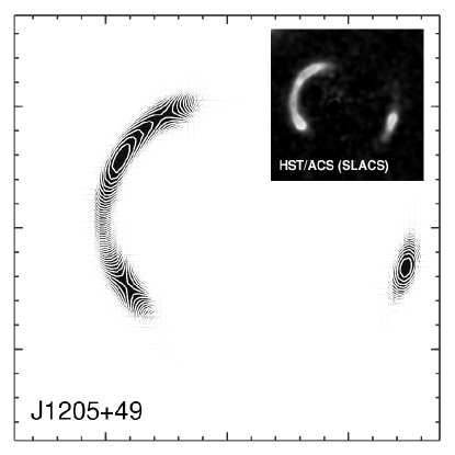
Figure 3: Extended images in the lens J1205+491. Main panel. Extended images predicted by our model for this lens, for a circular source of size $0.15^{\prime\prime}$ having a conical light profile. Inset. The observed image with the lensing galaxy substracted off.

3 Mapping the stellar mass

The galaxy images are Wide-Field Channel/ACS snapshots with an exposure time of 420s in each of the F435W ($B$) and F814W ($I$) filters. For each system we worked on the best-fit smooth lens-galaxy image that was originally subtracted from the actual image in order to discern faint lensing features. The lens-galaxy images were further corrected for Galactic reddening using the available dust maps (Schlegel et al., 1998) and a standard model for extinction by Galactic dust (Fitzpatrick, 1999). We then spatially rebinned the photometry of each galaxy into the same $21\times 21$ pixelation used for the lens models of that galaxy. These pixels are $\sim 0.1^{\prime\prime}$ to $0.2^{\prime\prime}$ across, depending on the system, amounting to $\sim 0.1$ to 1 kpc at the lensing galaxy.

For the stellar-population analysis we apply the so-called $\tau$ models, which assume an exponentially decaying star formation history at fixed metallicity. Three parameters describe each model: the formation epoch (i.e., when star-formation starts), the formation timescale and the metallicity. We explore a grid of $64\times 64\times 64$ models and allow in our estimates only those models whose photometry is compatible with the observations, treating the $21\times 21$ pixels described above as independent. One colour is not sufficient for an estimate of the stellar ages and metallicities, but is enough to constrain the stellar mass content, because of the wide spectral range covered by $B-I$. Figure 1 illustrates this point. In this figure we consider a Chabrier (2003) Initial Mass Function with formation epoch $z_{F}=2$ or $z_{F}=5$, viewed from $z=0.1$ or $0.5$. The stellar mass corresponds to a galaxy with apparent magnitude $\rm F814W=20$ at the labelled redshifts. The shaded regions show the range of $B-I$ as the metallicity varies in the range $-1<\log Z/Z_{\odot}<+0.3$ and the star formation timescale varies as $-1<\log\tau({\rm Gyr})<+1$. The uncertainty in ages and metallicities result in a $\sim 0.2$–$0.3$ dex uncertainty in the stellar mass content.

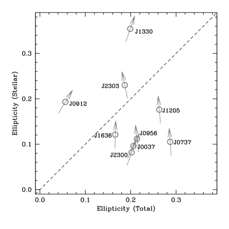
Figure 4: A comparison of the ellipticity of the total and stellar mass distributions. The dots give the values of the measured ellipticities whereas the orientation of the arrows represent the misalignment between both distributions; a vertical arrow means perfectly aligned.

Our sample comprises early-type galaxies. In these systems the presence of an overall old and coeval stellar population (Stanford et al., 1998) suggests star formation took place in a strong burst that consumed most of the available gas (Ferreras & Silk, 2003). Other baryonic components, hot and cold gas or dust, are known to contribute a small fraction to the net baryon budget in these systems (Roberts & Haynes, 1994). Hence, we can take the stellar mass content in each modeling pixel as the baryon content.

Table 1: Summary of the galaxy sample. (Indicated errors are 90% confidence.)

ID	$R_{e}^{1}$	Redshift1	$\sigma^{1}$	$R_{\rm M}$	M${}_{\rm TOT}(<R_{\rm M})$	M${}_{\rm STAR}(<R_{\rm M})$	$5\sigma^{2}R_{e}/G$
	kpc		km/s	$/R_{e}$	$10^{10}M_{\odot}$	$10^{10}M_{\odot}$	$10^{10}M_{\odot}$
J003753.21-094220.1	$6.99$	$0.195$	$265$	$1.66$	$52.3_{-14.5}^{+35.4}$	$44.3_{-4.3}^{+5.1}$	$57.1$
J073728.45+321618.5	$10.10$	$0.322$	$310$	$0.79$	$38.3_{-3.9}^{+11.8}$	$40.2_{-3.6}^{+4.1}$	$112.9$
J091205.30+002901.1	$9.47$	$0.164$	$313$	$0.95$	$71.2_{-21.7}^{+14.5}$	$44.7_{-4.0}^{+4.6}$	$107.9$
J095629.77+510006.6	$8.85$	$0.241$	$299$	$1.20$	$66.4_{-16.7}^{+25.7}$	$41.8_{-4.0}^{+4.9}$	$92.0$
J120540.43+491029.3	$8.03$	$0.215$	$235$	$1.04$	$38.6_{-5.5}^{+16.6}$	$50.5_{-4.6}^{+5.1}$	$51.6$
J133045.53-014841.6	$1.28$	$0.081$	$178$	$2.19$	$4.9_{-1.7}^{+3.5}$	$3.8_{-0.4}^{+0.4}$	$4.7$
J163602.61+470729.5	$5.41$	$0.228$	$221$	$2.01$	$52.9_{-14.3}^{+16.6}$	$32.2_{-3.2}^{+3.8}$	$30.7$
J230053.14+002237.9	$6.43$	$0.229$	$283$	$1.24$	$40.9_{-3.1}^{+14.2}$	$28.0_{-2.6}^{+3.0}$	$59.9$
J230321.72+142217.9	$8.13$	$0.155$	$260$	$1.17$	$49.8_{-15.5}^{+22.8}$	$37.5_{-3.5}^{+4.0}$	$63.9$

¹ Data from Bolton et al. (2006).

4 Comparison of stellar and total mass

With the methodology described in the previous two sections, we generated non-parametric 2D maps of the total and stellar surface density on the same pixelation. Figure 2 shows both distributions, the gray scale being $\Sigma_{\rm stel}$ derived from population synthesis and the contour maps indicating the $\Sigma_{\rm tot}$ derived from lensing. (Both maps have uncertainties, shown in later figures, but not here.) Seven of the lenses have the inversion-symmetry constraint mentioned in Section 2. For the two lenses where the images are well distributed in position-angle, J0912 and J1636, we did not impose inversion symmetry and the models are allowed to be lopsided. The asymmetry in these two lenses is at the level of 10–15% which given the uncertainties shown later in Figure 5 is probably not significant.

We noted in Section 2 that a model fitted to point-like features can be used to predict extended images to some degree. For one case this can be achieved with a simple piece of computer graphics. If one draws the arrival-time contours of the point source with a very close contour spacing, the resulting pattern models the lensed image of an extended source with a conical light profile (Saha & Williams, 2001). Figure 3 illustrates for one lens, J1205+491, which occupies the central panel of Figure 2. The white curves are the contour lines, and two minima and two saddle points are discernible; these are the locations of the point-like images. In most of the figure the contour lines are so close that the resulting pattern is almost completely white, and has been airbrushed out. In the region shown, however, the white-on-black pattern closely resembles the observed arcs. The white lines have width $w=0.01\;\rm arcsec$ on the scale of the figure. The contour spacing in scaled units (see e.g., Equation 2.3 in Blandford & Narayan, 1986) has been chosen as $\Delta\tau=0.0015\;\rm arcsec^{2}$. The implied source radius in this type of model is $\Delta\tau/w$ or $0.15^{\prime\prime}$. Koopmans et al. (2006) have much more detailed source maps (but much simpler lens models) and this source size is typical. The main conclusion from Figure 3 is that most of the lensing information in the extended images is already present in the point-like features.

Returning now to examine Figure 2 again, comparing the stellar and total mass profiles suggests that

1. $\Sigma_{\rm stel}$ and $\Sigma_{\rm tot}$ tend to have aligned ellipticity, and

2. $\Sigma_{\rm stel}$ falls off more steeply than $\Sigma_{\rm tot}$.

To test the statement (1) above, we compute the average ellipticity and position angle of $\Sigma_{\rm stel}$ and $\Sigma_{\rm tot}$ using the second order moments of the surface density. Figure 4 compares these. The orientations appear to be almost perfectly aligned. The tendency of lens models to be oriented with the light is well known (e.g., Keeton et al., 1997). At the same time, the magnitudes of the ellipticities is not correlated; in some galaxies the stellar part is rounder, in some galaxies the dark matter is rounder.

Statement (ii) above is addressed by Figure 5, which shows the circularly-averaged enclosed mass profiles, with 90% Bayesian confidence intervals. The error bars in the total mass derive from the ensemble of lens models, and have a characteristic butterfly (or bow-tie) shaped envelope as explained in Section 2. One envelope of the butterfly shape is expected to be approximately $M_{\rm tot}(R)\propto R^{1.5}$, because the prior requires $\Sigma_{\rm tot}$ to be steeper than $R^{-0.5}$ (see §2). This is indeed the case, as illustrated in the bottom-middle panel of the figure. The other envelope has a more complicated origin, having to do with the steepest non-negative profile that can reproduce the observed image positions. The uncertainty in the stellar mass arises from the variety of metallicities and star-formation histories compatible with the available photometry (see Figure 1). A Chabrier (2003) form for the IMF is assumed, with the effect of changing to a Salpeter IMF shown for one galaxy — we will return to this question below.

The strongest inference from Figure 5 is that dark matter is located in halos. While there is diversity in the details, the general pattern is that stellar mass dominates in the inner regions with the dark-matter fraction consistently increasing with radius. This conclusion is as expected based on our knowledge of stellar and gas dynamics in nearby galaxies, but is emerging here from a completely different method and data set.

Our sample spans a similar range of masses and velocity dispersion (see Table 1). Except for J1330, the total mass extends only over a factor of two. All galaxies appear baryon dominated at their centers, whereas outside the half-light radius the profiles show a wide range of distributions. Most of the galaxies show a significant contribution from dark matter. Interestingly, the only galaxy with no evidence of dark matter to the radius observed (J0737) is also the one where the observations are all interior of the half-light radius. This suggests that dark halos become significant roughly around the half-light radius.

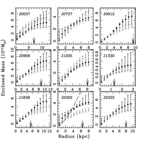
Figure 5: Cumulative mass profiles of the lensing galaxies. Black circles and grey triangles denote total and stellar mass, respectively. The error bars show the 90% confidence region. The effective radius ($R_{e}$; measured from the optical image) is given as an arrow for each galaxy. The enclosed mass is best constrained in the region of the images, with the error bars enlarging at smaller and larger radii. Outside of $R_{e}$ all the galaxies have a significant contribution from dark matter although some systems, most notably J2300, present a very high dark matter contribution. A Chabrier IMF is used for the stellar mass estimates. The grey crosses on the upper left panel correspond to the stellar mass for a Salpeter IMF, which gives an unphysical $\Sigma_{\rm tot}<\Sigma_{\rm stel}$ in the inner parts of the galaxy. The dashed curve in the bottom-middle panel shows $R^{1.5}$, the steepest enclosed-mass profile (equivalently shallowest density profile) allowed in our models. The normalization of the dashed curve is arbitrary.

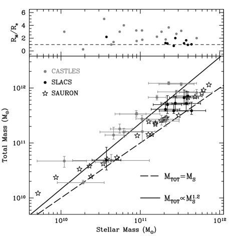
Figure 6: Stellar and total mass compared in lensing galaxies and in nearby galaxies with stellar dynamics. Main panel. Dots show the aperture masses $M_{\rm stel},M_{\rm tot}$. (The aperture is the region where the total mass is usefully constrained by lensing.) Black dots come from the present work using SLACS lenses, and gray dots from a similar analysis on a sample of CASTLES galaxies (Ferreras et al., 2005). The stars are measurements based on dynamical models applied to (non-lensing) elliptical galaxies observed with the SAURON Integral Field Unit (Cappellari et al., 2006). The dashed line corresponds to $M_{\rm tot}=M_{\rm stel}$, while the dashed line corresponds to $M_{\rm tot}\propto M_{\rm stel}^{1.2}$, which would give the observed tilt in the Fundamental Plane. Top panel. The aperture radius $R_{M}$ relative to the half-light radius $R_{e}$.

As mentioned above, we have assumed a Chabrier IMF for the stellar population, and other realistic choices of IMF differ from this one by a small factor not included in the error bars. The simple power law defined by Salpeter (1955) and traditionally used as an approximation to the IMF gives stellar masses $\sim 50\%$ higher. For some galaxies presented here, the implied stellar mass exceeds the total mass as extracted from lensing. The upper-left panel of figure 5 shows the stellar mass profile of J0037 for a Salpeter IMF, which is clearly incompatible with the lensing results. Hence, we can infer from our results that a Salpeter IMF is too bottom-heavy.

Our conclusion agrees with Cappellari et al. (2006), who used stellar dynamics to estimate the total mass in a sample of 25 E/S0 galaxies.

We can compare the aperture masses (stellar and total) with previous work. The aperture radius $R_{M}$ we take as $2R_{\rm max}-R_{\rm min}$, where $R_{\rm max}$ and $R_{\rm min}$ are the projected radii of the outermost and innermost lenses images. This $R_{M}$ approximates the radius within which lensing usefully constraints on the mass. In Ferreras et al. (2005) the aperture radius was set for each galaxy by seeing where the error bars became too large to be useful; such a procedure tends to give slightly smaller aperture radii, but we will disregard the difference here. Figure 6 shows the aperture $M_{\rm tot}$ and $M_{\rm stel}$ in this work along with the earlier lensing work (labelled CASTLES: Ferreras et al., 2005) and the stellar-dynamical work (labelled SAURON: Cappellari et al., 2006). The galaxies from these three independent data sets all show a clear trend towards a larger amount of dark matter in more massive galaxies. The observed tilt of the Fundamental Plane suggests a scaling of $M_{\rm tot}\propto M_{\rm stel}^{1.2}$ (Ferreras & Silk, 2000, 2003), which appears consistent with all the data. However, the present sample is too small to test a scaling law, especially because the range of aperture masses is small. Also noticeable in the figure is that the SLACS galaxies tend to have $R_{M}/R_{e}\simeq 1$, unlike the CASTLES galaxies which cover a larger range. This is a selection bias due to the SLACS survey strategy.

In Table 1 we include an estimate of the dynamical mass, using the popular relation $M_{\rm vir}=5R_{e}\sigma_{e}^{2}/G$ (e.g., Cappellari et al., 2006). In the table $R_{M}$ represents, as explained above, the aperture radius usefully mapped by lensing. Notice that for J0737 ($R_{M}=0.8R_{e}$) the dynamical mass estimate is much larger than the lensing or stellar masses within $R_{M}$, whereas J1330 ($R_{M}=2.2R_{e}$) is better mapped by the lensed images and give compatible results between $M_{\rm tot}$ and the dynamical mass.

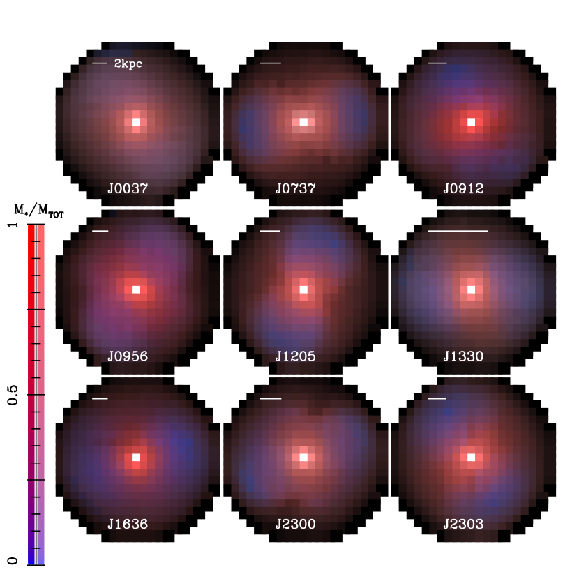
Figure 7: A false colour map of stellar and total mass in galaxies. The surface mass density is show by intensity (black: low density; bright: high density). Dark matter fraction is represented by colour (blue: dark matter dominated; red: stellar matter dominated). Uncertainty is encoded by hue (pale: high uncertainty, bright: low uncertainty). The colour bar on the left shows a range of mass ratios for two different uncertainties in the measurement of $\Sigma_{\rm stel}/\Sigma_{\rm tot}$: 0% (exact measurement; left) and 20% error (right). The horizontal bar in each panel indicates 2 kpc.

Finally, Figure 7 shows stellar and dark-matter maps in false colour. Here the brightness represents $\Sigma_{\rm stel}$; the colour represents the dark-matter fraction (red means all stellar, blue means all dark); the hue represents the uncertainty (pale means more uncertain). The Appendix explains the colour-coding scheme more precisely. At the centers of the galaxies we see bright white, meaning high density but with large uncertainty. This turns into pale red, indicating mainly stellar mass. Further out we see faint pale blue, indicating mainly dark matter. This figure, though admittedly ad hoc in its choice of colour coding, provides for the first time an intuitive visual image of the distribution of dark matter in individual galaxies.

5 Conclusions

The potential usefulness of early-type lensing galaxies for understanding the interdependence of baryons and dark matter in galaxy formation and evolution is widely appreciated. Lensing can be used to map the total mass and starlight can be used to map the baryons. In this paper we do this for nine galaxies from the SLACS survey by Bolton et al. (2006). From the lensing data we derived free-form pixelated models for the total mass, and from the galaxy photometry we computed stellar population-synthesis models. In both casses we generated Monte-Carlo ensembles of models, in order to marginalize over unknowns such as lensing degeneracies and star-formation histories, thus obtaining realistic uncertainties. The technique is basically the same as in Ferreras et al. (2005), but whereas the earlier work only compared radial profiles now we compare stellar and total mass in 2D. Related work has been done on larger samples of galaxies, but is limited to fitting simple parameterized models for the lens, and does not model the stellar populations at all.

The 2D mass maps are shown in Figures 2 and 7. The former overlays contours of $\Sigma_{\rm tot}$ on a grayscale of $\Sigma_{\rm stel}$. The latter shows the same information with uncertainties as well, all encoded in false colour: red for stellar mass, blue for dark, and pale versus coloured for uncertainty. It is evident that (a) these galaxies are dominated by stars in the inner regions, but mainly dark matter in the outer regions, and (b) stellar and dark components are well-aligned, but neither has a simple elliptical shape.

One can of course still compute an ellipticity defined as a moment, and this is shown in Figure 4. We see that ellipticities of the stellar and total mass are uncorrelated in magnitude but are almost perfectly aligned. It would be interesting to see if this is true of galaxy-formation simulations.

The profiles (Figure 5) show that dark matter halos begin to dominate around the half-light radius, although some galaxies seem to present a stronger contribution from dark matter even inside $R_{e}$ (e.g., J2300). The present sample is too small to extract any strong correlation of the dark matter distribution with global properties such as total mass or luminosity. However, the trend found previously (Ferreras et al., 2005), namely that there should be more dark matter in more massive galaxies, with a scaling of roughly $M_{\rm tot}\propto M_{\rm stel}^{1.2}$ (which is equivalent to the tilt of the Fundamental Plane) is compatible with the combined data of lensing galaxies (labelled CASTLES and SLACS) along with the dynamical analysis of local galaxies with the SAURON integral field unit (Cappellari et al., 2006).

The top-left panel of Figure 5 also shows that a Salpeter (1955) IMF cannot be used to estimate stellar masses as the population synthesis models predict too much stellar mass compared to the total mass obtained from our lensing studies. This result also agrees with the analysis of the SAURON sample.

We emphasize that stellar and total masses are obtained from different data through models of different physical processes. There is no tuning to give similar results. That the stellar and total densities come out compatible at the centers —where the baryon content is expected to dominate the mass budget— indicates that systematic effects are not significant.

Appendix A False-colour maps

For each galaxy we have sky-projected maps of three quantities: total mass, uncertainty, and stellar-mass fraction. How can we somehow encode these into red, green, and blue, thus making a false-colour map?

In general, suppose we want to represent the following three quantities:

$$A$$: an amplitude

$$f$$: a ratio of components (1)

$$\Delta$$: a fractional uncertainty

where $f$ and $\Delta$ both vary between 0 and 1. A plausible mapping into intensities $r,g,b$ of red, green, and blue is

$$r/A = {\textstyle\frac{1}{3}}\Delta+(1-\Delta)f$$

$$g/A = {\textstyle\frac{1}{3}}\Delta$$ (2)

$$b/A = {\textstyle\frac{1}{3}}\Delta+(1-\Delta)(1-f).$$

This gives total intensity $r+g+b=A$ regardless of $f$ and $\Delta$. If $\Delta=0$, the colour will vary from blue at $f=0$ to magenta at $f=0.5$ to red at $f=1$. As the uncertainty $\Delta$ increases, these colours will become paler, turning into white at $\Delta=1$.

The above scheme on its own is, however, not enough to produce useful false-colour maps. That is because the response of eyes to colour is highly nonlinear, contrary to what Equation (A) presupposes. In practical image-processing, heuristic scale stretchings are always necessary. After some experimentation, we found the stretchings

$$A=\Sigma_{\rm tot}^{1/2},\qquad f=\left(\frac{\Sigma_{\rm stel}}{\Sigma_{\rm tot}}\right)^{5/2},\qquad\Delta=\left(\frac{\Delta\Sigma_{\rm tot}}{\Sigma_{\rm tot}}\right)^{1/4}.$$ (3)

to be useful. $\Sigma_{\rm stel}$ and $\Sigma_{\rm tot}$ represent the surface mass density from the photometric and lensing analysis, respectively, in a given pixel. $\Delta$ is the fractional uncertainty in the total surface mass density, which dominates the error budget. Figure 7 shows the results.

References

- Binney et al. (1991) Binney, J., Gerhard, O. E., Stark, A. A., Bally, J., & Uchida, K. I. 1991, MNRAS, 252, 210
- Blandford & Narayan (1986) Blandford, R. & Narayan, R. 1986, ApJ, 310, 568
- Bolton et al. (2006) Bolton, A. S., Burles, S., Koopmans, L. V. E., & Moustakas, L. A. 2006, ApJ, 638, 703
- Brewer & Lewis (2006) Brewer, B. J. & Lewis, G. F. 2006, ApJ, 651, 8
- Bruzual & Charlot (2003) Bruzual, G. & Charlot, S. 2003, MNRAS, 344, 1000
- Cappellari et al. (2006) Cappellari, M., et al. 2006, MNRAS, 366, 1126
- Chabrier (2003) Chabrier, G. 2003, PASP, 115, 763
- Cretton & Emsellem (2004) Cretton, N. & Emsellem, E. 2004, MNRAS, 347, L31
- Dye & Warren (2005) Dye, S. & Warren, S. J. 2005, ApJ, 623, 31
- Ferreras et al. (2005) Ferreras, I., Saha, P., & Williams, L. L. R. 2005, ApJl, 623, L5
- Ferreras & Silk (2000) Ferreras, I. & Silk, J. 2000, MNRAS, 316, 786
- Ferreras & Silk (2003) Ferreras, I. & Silk, J. 2003, MNRAS, 344, 455
- Fitzpatrick (1999) Fitzpatrick, E. L. 1999, PASP, 111, 63
- Gerhard et al. (2001) Gerhard, O., Kronawitter, A., Saglia, R. P., & Bender, R. 2001, AJ, 121, 1936
- Keeton et al. (1997) Keeton, C. R., Kochanek, C. S., & Seljak, U. 1997, ApJ, 482, 604
- Keeton et al. (1998) Keeton, C. R., Kochanek, C. S., & Falco, E. E. 1998, ApJ, 509, 561
- Kochanek et al. (2000) Kochanek, C. S., et al. 2000, ApJ, 543, 131
- Koopmans (2005) Koopmans, L. V. E., 2005, MNRAS, 363, 1136
- Koopmans et al. (2006) Koopmans, L. V. E., Treu, T., Bolton, A. S., & Moustakas, L. A. 2006, ApJ, 649, 599
- Napolitano et al. (2005) Napolitano, N. R., et al. 2005, MNRAS, 357, 691
- Roberts & Haynes (1994) Roberts, M. S. & Haynes, M. P. 1994, ARA& A, 32, 115
- Rusin et al. (2003) Rusin, D., et al. 2003, ApJ, 587, 143
- Saha (2000) Saha, P. 2000, AJ, 120, 1654
- Saha & Williams (1997) Saha, P. & Williams, L. L. R. 1997, MNRAS, 292, 148
- Saha & Williams (2001) —. 2001, AJ, 122, 585
- Saha & Williams (2004) —. 2004, AJ, 127, 2604
- Saha, Williams & Ferreras (2007) Saha, P., Williams, L. L. R., & Ferreras, I. 2007, ApJ, in press, astro-ph/0703477
- Salpeter (1955) Salpeter, E. E. 1955, ApJ, 121, 161
- Schlegel et al. (1998) Schlegel, D. J., Finkbeiner, D. P., & Davis, M. 1998, ApJ, 500, 525
- Stanford et al. (1998) Stanford, S. A., Eisenhardt, P. R., & Dickinson, M. 1998, ApJ, 492, 461
- Suyu & Blandford (2006) Suyu, S. H. & Blandford, R. D., 2006, MNRAS, 366, 39
- Treu et al. (2006) Treu, T., Koopmans, L. V., Bolton, A. S., Burles, S., & Moustakas, L. A. 2006, ApJ, 640, 662
- Treu & Koopmans (2004) Treu, T. & Koopmans, L. V. E. 2004, ApJ, 611, 739
- Trotter et al. (2000) Trotter, C. S., Winn, J. N., & Hewitt, J. N. 2000, ApJ, 535, 671
- Valluri et al. (2004) Valluri, M., Merritt, D., & Emsellem, E. 2004, ApJ, 602, 66
- Wallington, Narayan & Kochanek (1994) Wallington, S. & Narayan, R., & Kochanek, C. S., 1994, ApJ, 426, 60
- White & Rees (1978) White, S. D. M. & Rees, M. J. 1978, MNRAS, 183, 341
- Williams & Saha (2000) Williams, L. L. R. & Saha, P. 2000, AJ, 119, 439
- York et al. (2000) York, D. G., et al. 2000, AJ, 120, 1579