On the effects of conformal degrees of freedom inside a neutron star

Abstract

In this paper a neutron star with an inner core which undergoes a phase transition, which is characterized by conformal degrees of freedom on the phase boundary, is considered. Typical cases of such a phase transition are e.g. quantum Hall effect, superconductivity and superfluidity. Assuming the mechanical stability of this system the effects induced by the conformal degrees of freedom on the phase boundary will be analyzed. We will see that the inclusion of conformal degrees of freedom is not always consistent with the staticity of the phase boundary. Indeed also in the case of mechanical equilibrium there may be the tendency of one phase to swallow the other. Such a shift of the phase boundary would not imply any compression or decompression of the core. By solving the Israel junction conditions for the conformal matter, we have found the range of physical parameters which can guarantee a stable equilibrium of the phase boundary of the neutron star. The relevant parameters turn out to be not only the density difference but also the difference of the slope of the density profiles of the two phases. The values of the parameters which guarantee the stability turn out to be in a phenomenologically reasonable range. For the parameter values where the the phase boundary tends to move, a possible astrophysical consequence related to sudden small changes of the moment of inertia of the star is briefly discussed.

Keywords: Junction conditions, Neutron Stars, Conformal Boundary Degrees of Freedom.
PACS: 04.40.Dg, 04.20.Jb, 26.60.+c, 11.25.Hf.
Preprint: CECS-PHY-07/20

1 Introduction

One of the most intriguing features of neutron stars is the possibility of having an inner core which undergoes a (colour) superconductivity and/or superfluidity phase transition due to the extremely high pressure and density. This fact was first pointed out by Migdal [1] (there is a huge amount of literature on this subject with a little hope of providing one with a complete list of references: for two detailed reviews, see [2] [3] and references therein; for general relativistic formalisms suitable for dealing with neutron stars within these scenarios see [4] [5] and references therein). Such phase transitions inside neutron stars could lead to interesting observational effects relevant in cosmology [6] and through the quasi normal modes of the stars as well as the related gravitational radiation (see, for instance, [7] [8]; detailed reviews on the subjects are [9] [10] [11]). Recently, there has been also pointed out the intriguing possibility to have a quantum hall phase of gluons and quarks in the inner core of a neutron star (see, in particular, [12] [13]). The discovery of magnetars [14], highly magnetized neutron stars whose magnetic fields can reach $10^{18}G$ in the core, makes the arising of Quantum Hall features in the inner core of a neutron star not unlikely. All the here described types of phase transitions have in common to be characterized by the presence of conformal degrees of freedom on the phase boundary predicted by QFT (see, for instance, [15] [16]).

The main goal of this paper is to study under which conditions the phase boundary inside a neutron star, which undergoes such a phase transition with conformal boundary degrees of freedom, can be static in general relativity, assuming mechanical equilibrium of the system. Indeed also if the system is mechanically stable i.e. there is no pressure inducing the collapse or expansion of the core, there can be another sort of instability: there may be the tendency of one phase to prevail over the other near the boundary. This would imply that the boundary gets shifted. This situation is analogous to a bubble chamber where a small perturbation induces a phase transition. To study this phenomenon one must take into account the contribution of the nontrivial traceless boundary stress tensor to the Einstein field equations. This problem is equivalent to solving Israel’s junction conditions. It is necessary to assume a dynamical phase boundary and to check under which conditions such a configuration is a solution of the Einstein field equations (by solving the junction conditions). It turns out that the equation of motion for the dynamical phase boundary is equivalent to the dynamics of a classical point particle in an effective potential. There exist a static stable equilibrium configuration if the effective potential has a local minimum for a suitable negative value of the potential. It is shown that the existence of a local minimum is regulated both by the difference in the mass density between the two phases and by difference of the slope of the two density profiles. A third parameter which determines the form of the potential is the energy of the shell. The non trivial effects of conformal boundary degrees of freedom have been pointed out, in the context of black hole physics, in [19] in which they are related to the arising (after the event horizon is formed) of Quantum Hall features [20] [15] related to the strong attractive nature of the gravitational field acting on Fermions inside a collapsed neutron star.

The structure of the paper is the following: in Section 2, the assumptions of the present paper are explained. In Section 3 the junction conditions derived from the Einstein equations for a neutron star with a phase boundary are solved. In section 4 the range of the physical parameters, characterizing our configuration, for which the phase boundary is in stable equilibrium is determined. In section 5 an astrophysical implication is discussed. Section 6 the conclusions and perspectives are drawn.

2 The standard approximations in a neutron star

Inside a neutron star, at the energy scale of the standard model of particle physics (up to $TeV$) the collapsing neutron star can be described very well by QFT and classical general relativity. The quantum dynamics of the neutrons and of the quarks living inside the neutron star is much faster than the dynamics of the gravitational field. This implies that one can compute the equation(s) of state of the Fermions as usual and then use such equation(s) to solve the Einstein equations in which the source is described by the equation of state itself. The success of this theory initiated by Landau, Chandrasekhar, Tolman, Oppenheimer, Volkoff, Snyder (and many others) tells that such an adiabatic approximation is excellent. The typical mass $M_{NS}$, radius $R_{NS}$, density $\rho_{NS}$ and the baryon number $N_{NS}$ a neutron star are

$$M_{NS} \approx 10^{33}g,\qquad R_{NS}\approx\left(10^{6}\div 10^{7}\right)cm,\text{ }$$

$$\quad\rho_{NS} \approx \left(10^{11}\div 10^{15}\right)g/cm^{3},\qquad N_{NS}\approx 10^{54}.$$

A neutron star pulsation can be thought of as a linearized solution of the Einstein equations around a background describing a static star (see, for the spherically symmetric case, Eq. (1)) with a ”quasi periodic” time dependence: that is, the perturbation $h_{\mu\nu}$ of the background metric Eq. (1) has the following form

$$h_{\mu\nu}\left(\overrightarrow{x},t\right)=\exp\left(i\left(\omega+\frac{i}{\tau}\right)t\right)h_{\mu\nu}^{\omega,\tau}\left(\overrightarrow{x}\right)$$

where the imaginary part of the frequency $\frac{1}{\tau}$ is due to the damping by emission of gravitational and electromagnetic waves (see, for instance, [9]). The standard order of magnitude of the frequency of a neutron star pulsation is

$$19,85\mathrm{Hz}\lessapprox\omega\lessapprox 12,84\mathrm{kHz}$$

while the damping has a wider range of possible values varying from low damping (in which $\tau$ can be of the order of years) to high damping (in which $\tau$ is of the order of millisecond).

3 Junction conditions and equation of motion of the phase boundary

In this section the junction conditions for the considered neutron star are found and the physical parameters that determine the existence of stable equilibrium configurations are found. We will set

$$\hbar=1,\qquad c=1,\$$

while keeping explicitly the Newton constant.

In the present case, one would like to describe a star in which the inner core underwent a gapped phase transition and therefore conformal boundary degrees of freedom localized at the separation between the two phases (predicted by QFT [15] [16]) have also to be included. We will therefore assume that there are two phases, each in mechanical equilibrium, namely the interior region which represents the exotic (superfluid, superconducting quantum Hall) phase and the exterior region which is the normal phase. Each phase is approximated by a perfect fluid in a static configuration. The two regions are characterised by very different equations of state.

We shall see that, even assuming static equilibrium (without any compression or decompression of the core), the conformally invariant matter living on the phase boundary may not be consistent with a static junction. In this case, since we assume that the conformal invariance is a defining characteristic of the phase transition, there must be some tendency of the phase boundary to move. Such a change in the position of the phase boundary is not by collapse of matter but by a kind of “creeping” phase transition, where one phase tends to swallow the other.

The metric describing a spherically symmetric neutron star can be parametrized as follows

$$ds^{2} =-\exp(2\nu)dt^{2}+\exp(2\lambda)dr^{2}+r^{2}d\Omega^{2}\,,$$ (1)

$$\nu =\nu(r),\ \ \ \lambda=\lambda(r)$$

where $d\Omega^{2}$ is the line element of a unit sphere. The functions $\nu$ and $\lambda$ are determined by the Einstein equations. If the source is a perfect fluid one gets the standard Tolman-Oppenheimer-Volkoff-Snyder equations:

$$\exp(2\lambda) = \left(1-2G\frac{m(r)}{r}\right)^{-1},\ \ \ m(r)=4\pi\int^{r}x^{2}\rho(x)dx$$ (2)

$$\partial_{r}P = -\left(\rho+P\right)\partial_{r}\nu,\ \ \ \ \partial_{r}\nu=\exp(2\lambda)\frac{\left(m+4\pi r^{3}P\right)}{r^{2}}$$ (3)

where $\rho$ and $P$ are the density and the pressure of the perfect fluid.

One has to find under which conditions such a configuration solves the Einstein field equations. Given the static perfect fluid solutions in the interior and exterior, this problem is equivalent to solving Israel’s junction conditions [21]. This technique allows the construction of an exact solution of the Einstein equations by matching two different solutions provided that the metric is continuous and the discontinuity of the extrinsic curvature is compensated by a suitable energy momentum tensor $S_{\mu}^{\nu}$ describing the boundary degrees of freedom of the inner phase: in the present case in which the inner phase transition is gapped one should only allow traceless $S_{\mu}^{\nu}$. Let $\Sigma$ be a timelike hypersurface of codimension one, on which the matching has to be performed. Let $n^{\mu}$ be the (spacelike) unit normal to $\Sigma$, and let $h^{\mu\nu}=g^{\mu\nu}-n^{\mu}n^{\nu}$ be the metric induced on $\Sigma$. The matching conditions at $\Sigma$ are: that the induced metric be continuous; that the jump in the extrinsic curvature is related to the intrinsic stress tensor localized on $\Sigma$ by [21]

$$\gamma_{\nu}^{\mu}=-8\pi G(S_{\nu}^{\mu}-\frac{1}{2}\delta_{\nu}^{\mu}trS),$$ (4)

where $\gamma_{\mu\nu}$ is defined as

$$\gamma_{\mu\nu}=\underset{\varepsilon\rightarrow 0}{\lim}\left[K_{\mu\nu}(\eta=+\varepsilon)-K_{\mu\nu}(\eta=-\varepsilon)\right]$$

$\eta$ being the arc length measured along the geodesic orthogonal to $\Sigma$. The extrinsic curvature $K_{\mu\nu}$ of $\Sigma$ is given by

$$K_{\alpha\beta}=h_{\alpha}^{\mu}h_{\beta}^{\nu}\nabla_{\mu}n_{\nu}\,.$$ (5)

In the present case, the matching is at a timelike hypersurface $r=r^{\ast}(\tau)$ (let us call such a surface $\Sigma_{(\tau)}$) which describes the time evolution of a thin spherical shell where the phase boundary occurs. Namely, at $r=r^{\ast}$ a gapped transition occurs (such as superconductivity, or Quantum Hall state).

3.1 The phase boundary

Because of the spherical symmetry, it can be assumed that the spatial sections of the timelike matching hypersurface $\Sigma_{(\tau)}$ are isomorphic to the two sphere so that there exist a coordinates system in which the induced metric $\left.ds^{2}\right|_{\Sigma_{(\tau)}}$ and $S_{\mu}^{\nu}$ respectively read:

$$\left.ds^{2}\right|_{\Sigma_{(\tau)}} = -d\tau^{2}+r^{2}(\tau)d\Omega^{2}$$

$$S^{\mu\nu} = \sigma(\tau)\left(U^{\mu}U^{\nu}\right)-\zeta\left(\tau\right)\left(h^{\mu\nu}+U^{\mu}U^{\nu}\right),$$ (6)

$$h^{\mu\nu} = g^{\mu\nu}-n^{\mu}n^{\nu}$$

where $h^{\mu\nu}$ is the metric induced on $\Sigma_{(\tau)}$, $n^{\mu}$ is the (spacelike) normal to $\Sigma_{(\tau)}$, $\tau$ is the arc length measured along the timelike geodesic belonging to $\Sigma_{(\tau)}$, $U^{\mu}$ is the normalized four velocity of $\Sigma_{(\tau)}$, $\sigma$ is the surface energy density of $\Sigma_{(\tau)}$, $\zeta\left(\tau\right)$ is the surface tension and the conservation of $S_{\mu}^{\nu}$ implies

$$\partial_{\tau}\sigma=-2(\sigma-\zeta)\frac{\partial_{\tau}r}{r}$$

with $r(\tau)$ being the proper circumferential radius of the domain wall $\Sigma_{(\tau)}$.The requirement of a traceless $S^{\mu\nu}$ (otherwise it would not correspond to the classical description of boundary gapless degrees of freedom) leads to

$$\sigma+2\zeta=0$$ (7)

which combined with the above conservation equation implies

$$\sigma=\frac{\sigma_{0}}{r^{3}},\qquad\sigma_{0}>0$$ (8)

where $\sigma_{0}$ is an integration constant, with the dimension of an energy times a length, which depends on the microscopic model and which will be approximated by a characteristic energy scale of the gapped phase transition times the length scale of the domain wall.

To get an intuition on the meaning of $\sigma_{0}$ let us consider the case in which in the inner core of the neutron star there is a Quantum Hall phase. In such a case, the only physical meaningful energy scale of the model is the energy gap $E_{gap}$, thus one can expect that

$$\sigma_{0}\approx\left(E_{gap}\sum_{i}^{n_{\max}}d(i)\right)r^{\ast}$$

where $r^{\ast}$ is a typical value of the radius of the inner core, the index $i$ labels the Landau levels, $d(i)$ is the degeneracy of the $i$-th level, and $n_{\max}$ is the last fully filled Landau level (so that $\sigma_{0}/\left(r^{\ast}E_{gap}\right)$ represents the number of particles living in the Hall phase). In the case of a supeconductivity/superfluidity phase inside the inner core also one should expect a close relation between $\sigma_{0}/r^{\ast}$ and the energy gap times a number of the order of magnitude of the number of particles living in the gapped phase.

The “equation of motion of the domain wall”, that is the equation which determines the evolution of $r(\tau)$, can be deduced from the matching condition (4). In particular, the important equation is the angular components $S_{i}^{i}$ of Eq. (4)

$$\gamma_{i}^{i}=-8\pi GS_{i}^{i}$$ (9)

One can see that the $\tau\tau$ component of the matching equations

$$\gamma_{\tau}^{\tau}=-8\pi GS_{\tau}^{\tau}$$ (10)

is not independent of the angular ones provided the consistency condition[21] $S^{\nu}_{\mu|\nu}=0\Rightarrow n^{\nu}T_{\mu\nu}(\text{ext})-n^{\nu}T_{\mu\nu}(\text{int})=0$ for the conservation of energy on $\Sigma$ is taken into account: one can easily see that the $\tau\tau$ component of the matching equations only constraints the discontinuity of the first derivative of the metric function $\nu$. Note that the pressure and density profiles are assumed to be static.

The standard procedure to compute $\gamma_{i}^{i}$ is as follows: the unit normal to the junction surface is

$$n_{\mu}=\pm\left(-\exp(\nu+\lambda)\partial_{\tau}r,\exp(2\lambda)\sqrt{\left(\partial_{\tau}r\right)^{2}+\exp(-2\lambda)},0,0\right)$$ (11)

where the $\pm$ ambiguity depends on whether one considers the inner or the outer directed unit normal. A straightforward calculation using (5) shows that the angular components of the extrinsic curvature is

$$K_{i}^{i}=\pm\frac{\sqrt{\left(\partial_{\tau}r\right)^{2}+\exp(-2\lambda)}}{r}$$ (12)

while the $\tau\tau$-component of the extrinsic curvature is ([22])

$$K_{\tau}^{\tau}=\pm\frac{\nu^{\prime}\left(\left(\partial_{\tau}r\right)^{2}+\exp(-2\lambda)\right)+\left(\partial_{\tau}^{2}r\right)+\lambda^{\prime}\left(\partial_{\tau}r\right)^{2}}{\sqrt{\left(\partial_{\tau}r\right)^{2}+\exp(-2\lambda)}}.$$ (13)

Eventually, Eq. (9) reads

$$\left(K_{i}^{i}(int)-K_{i}^{i}(ext)\right)=\frac{4\pi G\sigma_{0}}{r^{3}}\equiv\frac{K}{r^{3}}$$ (14)

where there is no sum on the repeated indices in this formula, $K_{i}^{i}(int)$ and $K_{i}^{i}(ext)$ stand for the extrinsic curvature computed on the inner and on the outer side of the junction. This equation can be written as an ordinary first order equation for $r(\tau)$ bringing on the right hand side $K_{i}^{i}(ext)$ and then squaring:

$$\left(\partial_{\tau}r\right)^{2}=\left[\frac{\left(\exp(-2\lambda_{int})-\exp(-2\lambda_{ext})\right)}{2K}r^{2}+\frac{K}{2r^{2}}\right]^{2}-\exp(-2\lambda_{ext})$$

which, using (2) can be written:

$$\left(\partial_{\tau}r\right)^{2}+V(r)=0\ ,$$ (15)

$$V(r)\equiv-\left(\frac{2Gm_{ext}(r)}{r}-1+\left[\frac{Gr}{K}(m_{ext}(r)-m_{int}(r))-\frac{K}{2r^{2}}\right]^{2}\right),$$ (16)

where $\lambda_{int}$ and $\lambda_{ext}$ stand for the metric functions of the inner and of the outer side of the junction and $m_{ext}(r)$ is the mass function (2) of the exterior part. It is worth to note an interesting feature of the present description: the dynamics of $r(\tau)$ given by equation (15) only depends on the metric function $\exp(-2\lambda)$ which in turns only depends on the density (see Eq. (2)).

The pressure inside and outside of the shell is given by the Tolman-Volkov-Oppenheimer-Snyder equations

$$\partial_{r}P = -\left(\rho+P\right)\left(1-2G\frac{m(r)}{r}\right)^{-1}\frac{\left(m+4\pi r^{3}P\right)}{r^{2}}$$ (17)

where $m$ and $\rho$ on each side are functions of $r$. Therefore we get an equation of the form $\partial_{r}P_{ext}a(r)+b(r)+c(r)P_{ext}(r)+d(r)P_{ext}^{2}(r)=0$ (and similarly for $P_{int}$), where $a$, $b$, $c$ and $d$ are polynomial in $r$, has a solution (which may be found numerically) with one constant of integration. For a consistent solution, we must take into account equation (10). To see the existence of a solution it is sufficient to consider the static case at the equilibrium radius $r_{eq}$, in which the equation reduces to:

$$\left[\frac{m(r_{eq})+4\pi r_{eq}^{3}P(r_{eq})}{r_{eq}^{2}\sqrt{1-\frac{2m(r_{eq})}{r_{eq}}}}\right]^{ext}_{int}=-2\frac{K}{r_{eq}^{3}}$$ (18)

where $[\cdots]^{ext}_{int}$ means the jump in this quantity across the shell. Generally, we can see this as an equation constraining the two integration constants for $P_{int}$ and $P_{ext}$ in terms of $K$. It is enough to know that there is a value for the pressure, but the precise value shall not be needed to solve the stability problem, since the potential depends explicitly on $\rho$ and not $P$.

One sees also that the equation of motion (15) for the shell $r(\tau)$ is formally analogous to the equation of motion of a classical point particle where $V(r)$ takes the role of an effective potential. A necessary condition to have a static phase boundary is that $V(r)$ must have a local minimum. The exact form of the potential depends now on the functional form of the density profiles of the two phases.

It will be now explicitly shown that in a suitable range of parameters such a local minimum exist.

4 Density profiles and (non)staticity of the phase boundary

To find the possible relative minima (if any) of the potential $V(r)$ one has to write explicitly $\lambda_{int}$ and $\lambda_{ext}$ as functions of $r$ and of phenomenological parameters characterizing the density of the star. At first glance, to do this one should solve the Tolman-Oppenheimer-Volkoff equations inside and outside the inner core. This is a very hard task since to do this one should approximate the equation of state of strongly interacting quarks, gluons, neutrons and so on at very high densities and pressures. In fact, this can be avoided: the reason is that the effective potential only depends on the metric functions $\lambda_{int}$ and $\lambda_{ext}$ (that is, on $g_{rr}$). Such function is expressed in terms of the density profile: if one is able to determine the dependence of the density on the radial coordinate $r$ the effective potential can be written explicitly. Remarkably enough, in many sound models of neutron stars it is possible to determine the density profile explicitly even if the knowledge of the equation of state (that is, the functional relation between density and pressure) is not perfect (see, for instance, [5] [10] [24] and references therein). On the basis of the above references, it will be here assumed that the density of the neutron star has the following form:

$$\rho_{int}(r) = \frac{A_{int}}{4\pi}-\frac{B_{int}}{4\pi}r^{n},\ \ \ r<r(\tau)$$ (19)

$$\rho_{ext}(r) = \frac{A_{ext}}{4\pi}-\frac{B_{ext}}{4\pi}r^{n},\ \ \ r>r(\tau),$$ (20)

where

$$n=1,\ \ A_{int},A_{ext}\approx\left(10^{11}\sim 10^{15}\right)g/cm^{3},\ \ \ B_{int},B_{ext}\approx\left(10^{11}\sim 10^{15}\right)g/cm^{4}.$$

Of course, even if it is not explicitly present, the pressure is needed to determine the values of the above density profiles. The choice of a linear decreasing is general enough since in the present case the important region is the one near the boundary phase so that a linear decreasing captures the main qualitative features (for instance, if one would take a quadratic decreasing (that is, $n=2$ in Eqs. (19) and (20)) as in [24] the main conclusions of the present paper would not change). On the other hand, interesting phenomenological conclusions can be reached in the cases in which further terms are added in the density profile. Such consequences will be discussed in a moment. Therefore, one can assume that both in the inner core ($r<r(\tau)$) and outside the core ($\ r>r(\tau)$) the density decreases linearly. With the above choice of the parameters the effective potential (16) reads

$$V(r) =-\bigg{(}2G\left(\frac{A_{ext}}{3}r^{2}-\frac{B_{ext}}{4}r^{3}\right)-1+\bigg{.}$$

$$\quad+\bigg{.}\frac{1}{r^{4}}\left[G\left(\frac{A_{ext}-A_{int}}{3K}\right)r^{6}-G\left(\frac{B_{ext}-B_{int}}{4K}\right)r^{7}+\frac{K}{2}\right]^{2}\bigg{)}\,.$$ (21)

To proceed, let us adopt the geometric unit of measure in which any quantity is expressed in powers of $cm$ (and the Newton constant is $1$):

$$1\ MeV\approx 10^{-55}cm,\qquad G=1\,.$$

Typical values are:

$$A_{ext} \approx 10^{-16}cm^{-2},\quad B_{ext}\approx 10^{-19}cm^{-3}\,,\qquad K\approx 10^{-29}cm^{2},$$

having assumed

$$E_{gap}\approx MeV,\ \ \ N\approx 10^{25},\ \ \ r^{\ast}\approx cm$$

where $N$ is the order of magnitude of the number of particles living in the inner phase and $r^{\ast}$ is the typical radius of the inner core.

4.1 Stable range

From a numerical analysis, it can be seen that in order for there to be a minimum of the potential we must have the following relations

$$\Delta A\Delta B>0,$$

a further condition is that

$$\left(\partial_{\tau}r\right)^{2}+V(r)=0\quad\Rightarrow\quad V(r)\leq 0.$$ (22)

When the above condition is not fulfilled, the Israel equations cannot be satisfied at all (the matching would be impossible). The numerical graphs also suggest that for a given $\Delta B$ there is a minimum value of $\Delta A$ below which solutions do not exist. For a core of radius $\approx 1\ cm$ this minimum is $\Delta A_{min}\approx\Delta B/2$ as shown in graph 2. More generally, one can check the following:

$$\Delta M=\frac{\Delta A}{3}r^{3}-\frac{\Delta B}{4}r^{4}\geq Kr^{2}\,.$$ (23)

This is natural (by analogy with special relativity) since $Kr^{2}$ is the rest mass of the shell and $\Delta m$ is a measure of the relativistic mass. If this condition is not fulfilled, there is either no minimum of the potential, or the minimum is positive, meaning no stable solution (see figure 2 ).

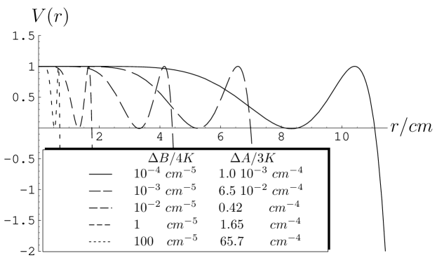
Figure 1: In this figure there is a graph of the effective potential for varying $10^{-4}cm^{-5}\leq\Delta B/4K\leq 100cm^{-5}$ and suitable values of $\Delta A/3K$ such that the potential has a minimum for small negative $V$. Stable solutions with radius of order $1-10$ $cm$ are shown to exist.

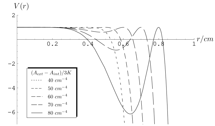
Figure 2: In this figure there is a graph of the effective potential for fixed $\Delta B/4K=100cm^{-5}$ and varying values of $\Delta A/3K$ (see plot legend above). Stable solutions exist for $\Delta A/3K$ greater than approximately $65cm^{-4}$.

In the range of parameters we focus on (see graph 1) a stable core exists: the equilibrium radius $r_{eq}$ and the frequency $\omega_{pul}$ are

$$r_{eq}\approx 0.53\ cm,\qquad\left.\partial_{r}^{2}V\right|_{r_{\min}}=146cm^{-2}\,,$$ (24)

$$r_{eq}\approx 1.32\ cm,\qquad\left.\partial_{r}^{2}V\right|_{r_{\min}}=23.1cm^{-2}\,$$

$$r_{eq}\approx 3.32\ cm,\qquad\left.\partial_{r}^{2}V\right|_{r_{\min}}=3.67cm^{-2}\,$$

$$r_{eq}\approx 5.26\ cm,\qquad\left.\partial_{r}^{2}V\right|_{r_{\min}}=1.46cm^{-2}\,$$

$$r_{eq}\approx 8.34\ cm,\qquad\left.\partial_{r}^{2}V\right|_{r_{\min}}=0.582cm^{-2}\,$$

So the frequencies are of order of GHz.

The above frequency of pulsation would correspond to a periodic motion of $r(\tau)$ between a maximum and a minimum radius oscillating around the above equilibrium radius. The equilibrium radius considered here is of the order of centimeters (which is in good agreement with the QFT estimates in the case of the Quantum Hall Effects [13] [12]; such a value for the radius of the inner core could also be compatible with the presence of a superconductivity/superfuidity phase [2] [3]).

4.2 Nonstatic range

The numerical analysis shows that if  $\Delta A$ and $\Delta B$ do not have the same sign the configuration is unstable: that is, the effective potential (21) has only one local maxima and the phase boundary will tend to move. It is important to stress that this result is a purely general relativistic effect related to the conformal boundary degrees of freedom. Such an effect would be overlooked if one neglects the possible dynamics of the phase boundary. If one construct a neutron star by matching the inner core and the outer part at a fixed radius $r^{\ast}=const$ (neglecting its possible dependence on $\tau$) and without the inclusion of the boundary degrees of freedom then it is not possible to disclose the effective potential.

4.3 Multiple equilibria?

As it has been already discussed, a density which decreases linearly with the radius is reasonable and general. On the other hand, it may be well possible (see [5] [10] and references therein) that the density profile is corrected by further terms as for instance

$$\rho_{int}(r) = \frac{A_{int}}{4\pi}-\frac{B_{int}}{4\pi}r+C_{int}r^{n},\ \ \ r<r(\tau)$$ (25)

$$\rho_{ext}(r) = \frac{A_{ext}}{4\pi}-\frac{B_{ext}}{4\pi}r+D_{ext}r^{m},\ \ \ r>r(\tau),$$ (26)

$$n,m > 1.$$ (27)

At a first glance, one could expect that near the phase boundary only the first two terms in Eqs. (25) and (26) are important. However, if due to the extreme conditions inside a neutron star, such further terms have to be taken into account, then interesting phenomenological scenarios open up. In these cases, the effective potential may have multiple local minima and the valleys would be generically asymmetric: namely the valley corresponding to the larger radius of equilibrium could be more deep than the valley corresponding to the smaller radius of equilibrium. In principle, a phase transition could occur in which the phase boundary jumps from one valley to the other.

5 Astrophysical Implication

From the explicit form of the effective potential (21) it is clear that, in the range of parameters in which the effective potential has a local minimum, it is consistent to assume a static phase boundary. In this range of parameters also small oscillations of the phase boundary could be possible. However it is difficult to say what would be the sources of dissipation which would damp the oscillations.

It is a well known fact since the Migdal paper [1] that the presence of a superfluid phase inside a neutron star affects its moment of intertia. In the range of parameters in which the phase boundary tends to move one phase tends to swallow the other. In the case in which the inner phase expands, there is a corresponding decrease of the moment of intertia. Assuming that our results also hold for the rotating case (which is a reasonable assumption at least in the slow rotating case [10] [26]) this would lead to interesting observable effects: namely a sudden small increase of the angular velocity because of the angular momentum conservation. Analogously, in the case in which the inner phase shrinks, there is a corresponding decrease of the angular velocity. Indeed both types of phenomena are of interest in astrophysics.

6 Conclusions and perspectives

We have studied a model of a neutron star with an inner core which undergoes a phase transition. It has been shown that, even assuming mechanical equilibrium, it is not always consistent to assume a static phase boundary once conformal boundary degrees of freedom are taken into account.

In order to study the staticity of such a phase boundary one must take into account the general relativistic effects of these boundary degrees of freedom by including a nontrivial stress tensor on the junction. To the best of the authors knowledge, such a consistency analysis with conformal boundary degrees of freedom has not been performed previously. The astrophysical consequences of the non-static regime, related to sudden changes of the moment of inertia of the star, are worth further investigating.

References

- [1] A. B. Migdal, Nucl. Phys. 13 (1959) 655.
- [2] C. J. Pethick, Rev. Mod. Phys. 64 (1992), 1133.
- [3] M. Alford, J. A. Bowers, K. Rajagopal, J.Phys. G27 (2001) 541; Lect.Notes Phys. 578 (2001) 235.
- [4] B. Carter, D. Langlois, Nucl.Phys. B531 (1998) 478.
- [5] N. Andersson, G. L. Comer, ”Relativistic Fluid Dynamics: Physics for Many Different Scales”; Living Rev. Relativity 10, (2007), 1.
- [6] G. Sigl, JCAP 0604, 002 (2006) [arXiv:astro-ph/0602345].
- [7] H. Sotani, K. Tominaga, K. Maeda, Phys.Rev. D65 (2002) 024010.
- [8] G. Miniutti, J. A. Pons, E. Berti, L. Gualtieri, V.Ferrari, Mon. Not. Roy. Astron. Soc. 338 (2003) 389.
- [9] K. D. Kokkotas, B. Schmidt, ”Quasi-Normal Modes of Stars and Black Holes”, Living Rev. Relativity 2, (1999), 2.
- [10] N. Stergioulas, ”Rotating Stars in Relativity”, Living Rev. Relativity 6, (2003), 3.
- [11] M. Sasaki, H. Tagoshi, ”Analytic Black Hole Perturbation Approach to Gravitational Radiation”, Living Rev. Relativity 6, (2003), 6.
- [12] A. Iwazaki, O. Morimatsu, M. Ohtani, T. Nishikawa, Phys.Rev. D71 (2005) 034014.
- [13] A. Iwazaki, Phys. Rev. D 72, 114003 (2005); hep-ph/0604222.
- [14] R.C. Duncan and C. Thompson, Astrophys. J. Lett. 392, L9 (1992); C. Thompson and R.C. Duncan, Astrophys. J. 408, 194 (1993); C. Thompson and R.C. Duncan, MNRAS 275, 255 (1995); C. Thompson and R.C. Duncan, Astrophys. J. 473, 322 (1996).
- [15] F. Wilczek, Fractional Statistics and Anyon Superconductivity, World Scientific (1990).
- [16] S. Weinberg, The Quantum Theory of Fields, Vol II, Cambridge University Press (1996).
- [17] J. Ellis, J. I. Kapusta, K. A. Olive, Nuclear Physics B 348, (1991) 345.
- [18] M. Alford, J. Berges, K. Rajagopal, Nucl.Phys. B571 (2000) 269.
- [19] F. Canfora ”Incompressible fluid inside an astrophysical black hole?” arXiv:0707.2768 to appear on Phys. Rev. D.
- [20] R. B. Laughlin, Rev. Mod. Phys. 71 (1999), 863.
- [21] W. Israel, Nuovo Cimento 44B, 1 (1966); 48B, 463(E) (1967).
- [22] H. Sato, Prog. Theor. Phys. 76, 1250 (1986).
- [23] S. K. Blau, E. I. Guendelman, A. H. Guth, Phys. Rev. D35 (1987), 1747.
- [24] J. M. Lattimer, M. Prakash, Phys.Rept. 333 (2000) 121.
- [25] P. K. Sahu, G. F. Burgio, M. Baldo, The Astrophysical Journal, 566 (2002), L89.
- [26] V. Ferrari, L. Gualtieri, S. Marassi, ”A new approach to the study of quasi-normal modes of rotating stars” arXiv:0709.2925.