Efficient algorithms for rigid body integration using optimized splitting methods and exact free rotational motion

In this note we present molecular dynamics integration schemes that combine optimized splitting and gradient methods with exact free rotational motion for rigid body systems and discuss their relative merits. The algorithms analyzed here are based on symplectic, time-reversible schemes that conserve all relevant constants of the motion. It is demonstrated that although the algorithms differ in their stability due to truncation errors associated with limited numerical precision, the optimized splitting methods can outperform the commonly-used velocity Verlet scheme at a level of precision typical of most simulations in which dynamical quantities are of interest. Useful guidelines for choosing the best integration scheme for a given level of accuracy and stability are provided.

Hamiltonian splitting methods are an established technique to derive stable and accurate integration schemes in molecular dynamics.splitting The strategy of these methods is to split the Hamiltonian of the system into parts whose evolution can be solved exactly. Using the Campbell-Baker-Hausdorff formulacbh , splitting algorithms can be presented as products of exactly solvable propagation steps, involving more factors for higher-order schemes.ForestRuth The resulting algorithms can be optimized by adjusting the form of the splitting to minimize error estimates.Omelyan1

Recently, second- and fourth-order symplectic integration schemes for simulations of rigid body motion, based on the exact solution for the full kinetic (free) propagator, have been proposed.us1 While this exact solution involves elliptic functions, elliptic integrals and theta functions,Jacobi1849 there exist efficient numerical routines to compute elliptic functions,gsl and the computation of elliptic integrals and theta functions can be implemented efficientlyus2 or avoided altogether using a recursive method.us1 Employing the exact free rotational motion, the resulting splitting method leads to demonstrably more accurate dynamics for systems in which free motion is important.us1 Furthermore, using the exact kinetic propagator, any splitting scheme for integrating the dynamics of point particles can be transferred to rigid systems. Here we analyze the combination of the exact kinetic propagator and optimized splitting and gradient-likeOmelyan1 ; Omelyana ; Omelyan2 approaches.

For a system of rigid bodies, a phase space point $\Gamma$ is specified by a center of mass position $\mathbf{q}_{i}$, an attitude matrix $\mathsf{S}_{i}$, and translational and angular momenta $\mathbf{p}_{i}$ and $\bm{\ell}_{i}$ for each particle $i$ of mass $m_{i}$. Given the Hamiltonian $H=T+V$, where $T$ and $V$ are the kinetic and potential energies, respectively, the time evolution of the point $\Gamma$ in phase space is governed by $\dot{\Gamma}=\{H,\Gamma\}=\{T,\Gamma\}+\{V,\Gamma\}$, in which $\{,\}$ denotes the Poisson bracket. Henceforth, the operators $\{T,.\}$ and $\{V,.\}$ will be designated as $A$ and $B$, respectively. Defining $\mathcal{L}$ = $A+B$, the solution of the equations of motion is formally given by $\Gamma(t)=e^{\mathcal{L}t}\Gamma(0)$.

While the various possible splitting schemes can be assigned a theoretical efficiency,Omelyan1 the relative efficiency of real simulations can be somewhat different. Nonetheless, the estimates are useful to eliminate the least efficient variants. Based on our studies of second and fourth order methods, the most efficient integration schemes can be formulated using the following generic form of the splitting algorithm for a single time step of size $h$:

$$e^{\mathcal{L}h}=e^{\eta Bh}e^{Ah/2}e^{(1-2\eta)\hat{B}(\xi)h}e^{Ah/2}e^{\eta Bh}+\mathcal{O}(h^{k+1}).$$ (1)

This propagator is applied $t/h$ times to compute the time evolution of the system over a time interval $t$. Here, $\eta$ and $\xi$ are two real parameters, $k$ is the order of the integration scheme, and $e^{Ah}$ and $e^{Bh}$ act on a phase space point $\Gamma=\{\mathbf{q}_{i},\mathbf{p}_{i},\mathsf{S}_{i},\bm{\ell}_{i}\}$ as

$$e^{Ah}\Gamma = \{\mathbf{q}_{i}+h\mathbf{p}_{i}/m_{i},\mathbf{p}_{i},\mathsf{P}_{i}(h)\mathsf{S}_{i},\bm{\ell}_{i}\},$$ (2)

$$e^{Bh}\Gamma = \{\mathbf{q}_{i},\mathbf{p}_{i}+h\mathbf{f}_{i},\mathsf{S}_{i},\bm{\ell}_{i}+h\bm{\tau}_{i}\},$$ (3)

where $\mathbf{f}_{i}$ and $\bm{\tau}_{i}$ are the instantaneous forces and torques on body $i$, while the matrix $\mathsf{P}_{i}(h)$ propagates exactly $\mathsf{S}_{i}$ over the time interval $h$ in the absence of torques [see Ref. us1, for specific forms for $\mathsf{P}_{i}(h)$]. Finally, $\hat{B}(\xi)$ in Eq. (1) is a variation of $B$ which takes the gradients of forces and torques into account by an advanced gradient-like method.Omelyan2 More precisely, the action of $e^{\hat{B}(\xi)h}$ on a phase space point is given by

$$e^{\hat{B}(\xi)h}\Gamma=\{\mathbf{q}_{i},\mathbf{p}_{i}+h\tilde{\mathbf{f}}_{i},\mathsf{S}_{i},\bm{\ell}_{i}+h\bm{\tilde{\tau}}_{i}\},$$ (4)

where the modified forces $\tilde{\mathbf{f}}_{i}$ and torques $\bm{\tilde{\tau}}_{i}$ areOmelyan2

$$\tilde{\mathbf{f}}_{i}=\mathbf{f}_{i}+\Delta\mathbf{f}_{i}(\xi,\lambda),\quad\bm{\tilde{\tau}}_{i}=\bm{\tau}_{i}+\Delta\bm{\tau}_{i}(\xi,\lambda).$$ (5)

The shifts in forces and torques account for commutator corrections involving gradients.Omelyan2 To fourth order in $h$, the shifts can be approximated by a finite difference approach using a small parameter $\lambda$ according to

$$\Delta\mathbf{f}_{i}(\xi,\lambda) = [\mathbf{f}_{i}(\tilde{\mathbf{q}},\tilde{\mathsf{S}})-\mathbf{f}_{i}(\mathbf{q},\mathsf{S})]/\lambda,$$

$$\Delta\bm{\tau}_{i}(\xi,\lambda) = [\bm{\tau}_{i}(\tilde{\mathbf{q}},\tilde{\mathsf{S}})-\bm{\tau}_{i}(\mathbf{q},\mathsf{S})]/\lambda,$$

where $\mathbf{f}_{i}(\tilde{\mathbf{q}},\tilde{\mathsf{S}})$ and $\bm{\tau}_{i}(\tilde{\mathbf{q}},\tilde{\mathsf{S}})$ are the forces and torques at the auxiliary coordinates

$$\tilde{\mathbf{q}}_{i}=\mathbf{q}_{i}+2\xi\lambda h^{2}\mathbf{f}_{i}/m_{i},\quad\tilde{\mathsf{S}}_{i}=\mathsf{R}(2\xi\lambda h^{2}\mathsf{J}^{-1}_{i}\mathsf{S}_{i}\bm{\tau}_{i})\mathsf{S}_{i}.$$ (7)

Here, $\mathsf{J}_{i}$ is the diagonalized moment of inertia tensor of the $i$th body [i.e. $\mathrm{diag}(I_{1},I_{2},I_{3})$] and $\mathsf{R}(\mathbf{v})$ is the Rodrigues matrixGoldstein that performs a rotation around a vector $\mathbf{v}$. Note that for $\xi=0$, $\hat{B}(0)=B$, in which case there are no advanced-gradient contributions. Although the finite difference approach introduces non-symplectic terms of order $\lambda^{2}h^{4}$, no discernible energy drift was found for small integration time steps $h$ when the value of the parameter $\lambda$ was taken to be roughly $10^{-4}$.Omelyan2

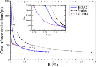
Figure 1: Efficiency of integration schemes for simulations of rigid water. For various values of the timestep $h$, the plot shows the relative error versus cost (in force evaluation per ps). The plots extend up to values of $R$ where the simulations start to exhibit statistically-significant drift due to numerical round-off. The inset shows the same on a logarithmic scale.

By tuning the parameters $\xi$ and $\eta$, different integration schemes can be obtained. Choosing $\xi=0$ and $\eta=0$ or $\eta=1/2$ results in the well-known second-order ($k=2$) Verlet scheme, in its position or velocity form, respectively. Fixing $\xi=0$ but allowing $\eta$ to vary, the prefactors can be minimized in front of the $\mathcal{O}(h^{2})$ corrections, which gives $\eta=0.1931833275037836$ as an optimal choice. Omelyan1 ; Omelyan2 This scheme, which was called HOA2 in Ref. Omelyan2, , is still second order but is expected to be more accurate. Finally, one can vary both $\eta$ and $\xi$, to make the prefactors of the $\mathcal{O}(h^{2})$ corrections vanish to yield a fourth-order algorithm. Omelyan2 For this scheme, which we have called GIER4, the required values are $\eta=1/6$ and $\xi=1/48$.

To assess the relative computational cost of each of the integration schemes at a given level of accuracy, simulations of 512 rigid water molecules using the TIP4P potentialTIP4P were carried out at liquid density of 1 g/cm³ and a temperature of 297 K. The accuracy of the simulations was measured by calculating the ratio $R$ of fluctuations of the total energy to the fluctuations of the potential energy at a given computational load. This load was estimated by using the number of force evaluations in a given time interval, here taken to be 1 picosecond (ps). At liquid densities, the computational load correlates very well with the overall CPU time since relatively little CPU time is required in the free motion propagation steps. In addition, the stability of each integration scheme was monitored by a linear least-squared analysis of the drift of the total energy over a series of 10 to 50 runs of total length $15$ ps for each time step reported.

The results of this analysis are plotted in Fig. 1, from which it is evident that for crude simulations requiring only modest energy conservation (i.e. $R>1.5\%$), the standard Verlet algorithm is the only algorithm that is stable. Trajectories at this level of accuracy can be used in sampling schemes such as hybrid Monte-Carlo. However for $R<1.5\%$, arguably the upper limit of allowable error in simulations from which dynamical information can be extracted, the optimized second-order HOA2 scheme is roughly $1.5$ times more efficient than the Verlet algorithm. Note that the HOA2 algorithm differs from the velocity Verlet scheme only in the choice of time step for the momenta updates and is therefore simple to implement. Interestingly, the fourth order GIER4 scheme is preferable if very accurate simulations are required ($R<0.4\%$) in spite of the additional computational cost of the modified forces and torques at auxiliary positions. Other fourth-order splitting schemesOmelyan1 (not outlined here) have also been tested and found to be less efficient than the relatively simple GIER4. Streamlining explicit calculations of the gradients of forces and torques instead of utilizing finite difference methods would restore symplecticity and likely increase the value of $R$ at which the GIER4 method is optimal.

Acknowledgments: R.v.Z. and J.S. acknowledge support by a grant from NSERC and a PRF (ACS) grant. I.O. thanks the Fonds zur Förderung der wissenschaftlichen Forschung (project No. 18592-PHY).

References

- (1) B. Leimkuhler and S. Reich, Simulating Hamiltonian Dynamics (Cambridge University Press, Cambridge, 2005).
- (2) G. Parisi, Statistical Field Theory (Addison-Wesley, Reading, MA, 1988).
- (3) E. Forest and R.D. Ruth, Physica D 43, 105 (1990).
- (4) I. P. Omelyan, I. M. Mryglod, and R. Folk, Comp. Phys. Comm. 151, 272 314 (2003).
- (5) R. van Zon and J. Schofield, Phys. Rev. E 75, 056701 (2007).
- (6) C.G.J. Jacobi, Crelle J. Reine Angew. Math. 39, 293 (1849).
- (7) M. Galassi, J. Davies, J. Theiler, B. Gough, G. Jungman, M. Booth, and F. Rossi, GNU Scientific Library Reference Manual (Network Theory Ltd, Bristol, UK, 2005), revised 2nd ed.
- (8) R. van Zon and J. Schofield, J. Comput. Phys. 225, 145 (2007).
- (9) I.P. Omelyan, Phys. Rev. E 74, 036703 (2006).
- (10) I.P. Omelyan, J. Chem. Phys. 127, 044102 (2007).
- (11) H. Goldstein, Classical Mechanics (Addison-Wesley, Reading, Massachusetts, 1980).
- (12) W.L. Jorgensen, J. Chandrasekhar, J.D. Madura, R.W. Impey, and M.L. Klein, J. Chem. Phys. 79, 926 (1983).