The ’t Hooft Model As A Hologram

Abstract:

We consider the 3d dual of $1+1$ dimensional large-$N_{c}$ QCD with quarks in the fundamental representation, also known as the ’t Hooft model. ’t Hooft solved this model by deriving a Schrödinger equation for the wavefunction of a parton inside the meson. In the scale-invariant limit, we show how this equation is related by a transform to the equation of motion for a scalar field in AdS₃. We thus find an explicit map between the ‘parton-$x$’ variable and the radial coordinate of AdS₃. This direct map allows us to check the AdS/CFT prescription from the 2d side. We describe various features of the dual in the conformal limit and to the leading order in conformal symmetry breaking, and make some comments on the 3d theory in the fully non-conformal regime.

1 Introduction

Our limited understanding of gauge theory dynamics in the non-perturbative regime hampers both our description of QCD phenomena, as well as our ability to construct viable scenarios with strong dynamics for physics beyond the Standard Model. Lattice theory has been helpful in addressing some of the issues, however it does face certain challenges. Some of these difficulties include treatment of time evolution in a system with temperature or chemical potential, simulation of supersymmetric theories, and dealing with chiral symmetry in an efficient manner. Thus, it is desirable to find novel theoretical tools to tackle non-perturbative physics. The AdS/CFT framework [1] offers a different approach for performing calculations in field theory in the non-perturbative regime. The local operators of the original field theory are mapped to fields propagating in a curved higher-dimensional background. A general field theory contains a multitude of local operators, and therefore its higher-dimensional dual is expected to contain infinitely many fields. The interactions of these higher-dimensional fields, which can be of large spin, are expected to be quite complicated, and in general are difficult to determine. Considerable simplification occurs when the field theory admits a limit for which most of the operators acquire large anomalous dimensions. The anomalous dimensions are mapped via AdS/CFT to masses of the dual higher-dimensional fields, and thus such a limit effectively decouples most fields. The remaining fields are usually those dual to operators whose dimensions are protected by various symmetries. These are typically duals of currents (and possibly their superpartners), and their interactions are heavily constrained by symmetry. Thus, most known duals are of theories where there is a significant hierarchy between the dimensions of operators. Unfortunately, this is not the case for QCD, which is partly why it has thus far been difficult to construct its dual, though duals to other field theories with ‘QCD-like’ dynamics have been found. In a few cases it has been possible to find soluble higher-dimensional string duals to certain field theories (or sub-sectors thereof)[2]. Such descriptions capture effectively the physics of many higher-dimensional fields (the resonances of the string), going beyond the limited set constrained by symmetry. One may hope that a theory like QCD admits such a string description, however thus far, none has been found.

Hence, instead of attempting to find a dual to the full QCD theory, it might be fruitful to consider only a limited set of operators, and find a description for their holographic dual fields. Such an approach faces certain obvious challenges. The first is that one would expect that any operator has non-trivial correlation functions with many other operators (as allowed by symmetry and Lorentz invariance), and thus its dual field will necessarily interact with many other fields. As mentioned, these interactions are difficult to determine and usually are not even renormalizable. However, in the limit of large number of colors, $N_{c}$, all interactions are suppressed, and one is left with a quadratic action of free fields propagating on some background. One may worry that such an action includes higher-derivative terms. After all, there is no parameter in QCD, such as the ’t Hooft coupling, that would suppress them. However, leading $1/N_{c}$ calculations correspond to ‘on-shell’ calculations in the higher-dimensional theory, and thus only care about the dispersion relation governing the propagation of the dual field in the curved background. If we know the background exactly and include all (typically an infinite number of) fields, then in principle we can find a basis of fields where dispersion relations become quadratic in derivatives, hence the action is local in this sense. Thus, if we limit ourselves to asking questions that concern only the quadratic part of the action (i.e. focus on masses, decay constants, and two-point functions), this approach may be useful. Finally, there is the question of the curved background itself. In the UV QCD is asymptotically free, and therefore the background should approach AdS. Thus, a natural place to start is the conformal limit of QCD, for which we know much more about the quadratic action. Indeed, 4d Poincaré invariance tells us that the dispersion relation is quadratic in 4d momenta, so derivatives with respect to 4d coordinates enter quadratically in the action. The AdS isometry then guarantees that derivative along the 5th coordinate also enters quadratically. This plus the usual consideration of internal symmetries, etc. completely fixes the form of the quadratic action (at least for propagating fields). In addition, we need only consider the duals of primary operators as their descendents are automatically included by the AdS isometry. As primary operators do not mix, this is a basis of for bulk fields for which the quadratic action becomes diagonal.

The simplicity will be lost once we take into account the effects of conformal symmetry breaking, such as the running QCD coupling, confinement, chiral symmetry breaking, etc. Such effects can be parameterized in terms of various backgrounds in the higher-dimensional space. Denoting the 5th coordinate by $z$, these background in general depend on $z$. Then, it is no longer true that the quadratic 4d dispersion implies that $\partial_{z}$ appears quadratically in the action. For example, suppose we are interested in the quadratic action for a scalar field $\phi$ and there is a background of another scalar field $\Phi$ parameterizing some conformal symmetry breaking effects. In the full action, there might be a term like $g^{M_{1}N_{1}}g^{M_{2}N_{2}}g^{M_{3}N_{3}}g^{M_{4}N_{4}}(\partial_{M_{1}}\Phi)(\partial_{M_{2}}\Phi)(\partial_{M_{3}}\Phi)(\partial_{M_{4}}\Phi)(\partial_{N_{1}}\partial_{N_{2}}\phi)(\partial_{N_{3}}\partial_{N_{4}}\phi)$. Once a $z$-dependent $\Phi$ background is turned on, this yields a quadratic term for $\phi$ with four $\partial_{z}$’s. Therefore, away from the exact AdS, we do not know how many $z$ derivatives are in the action. Also, a term like $\Phi^{2}\phi^{2}$ will give us a $z$-dependent mass term for $\phi$. In addition, conformal symmetry breaking will generally induce mixing between fields corresponding to operators with different scaling dimensions. But as mentioned above, these higher derivative terms are merely a consequence of integrating out heavier fields which mix with $\Phi$. Once we ‘integrate in’ all fields and include all the mixings among them, there should be a basis for the fields for which the quadratic action is local.

The above complexity means that it may be difficult to derive the dual of QCD but we might at least learn something about the full theory. Restricting to a regime where QCD is almost conformal (i.e. looking at the correlators at large Euclidean momenta), we can match the (small) conformal breaking effects order-by-order in $\Lambda_{\rm QCD}$. This tells us how the backgrounds affect the quadratic Lagrangian at small $z$ (the UV of theory). This knowledge may be sufficient for certain questions. If for example, a particular bulk mode profile is localized sufficiently far from the large $z$ region, then the details of conformal symmetry breaking might not be very important in determining its properties.

The above philosophy is the motivation for the ‘AdS/QCD’ phenomenological approach which has been applied to fields of various spin [3] [4] [5]. A good agreement of masses and decay constants with data is found. This is an indication that for low-lying KK-modes, both the large $N_{c}$ approximation works remarkably well, and the profile of KK-modes is surprisingly well described by assuming the background is close to AdS with a hard cutoff. Still, it is clear that such a description is naive as it does not capture the spectrum of the highly excited modes, which lie on Regge trajectories. A simple model which captures the Regge spectrum was presented in [6], but its origin remains unclear. In particular, as mentioned, once conformal symmetry is broken, all fields dual to operators of similar quantum numbers are expected to mix in a complicated way. It is therefore a mystery why this mixing is effectively captured by the simple diagonal action of [6].

In this paper we will attempt to test the AdS/QCD approach in a simpler setting where there is some analytic control over the non-perturbative dynamics. In particular, we will focus on two-dimensional QCD in the large $N_{c}$ limit. The spectrum of this model was solved by ’t Hooft [7], who derived a Schrödinger equation for the meson wavefunction (as a function of the parton-$x$ variable). While one could “build” a 3d AdS/QCD model with a few fields propagating in some effective background chosen to reproduce the meson spectrum, that is not the goal of this paper. As mentioned above, our view is that such 3d model is an approximation of the (quadratic) action involving an infinite number of fields mixed with each other, corresponding to the infinite number of operators mixed with each other on the 2d side. Our goal is to understand such mixings and how they are mapped between 2d and 3d, taking advantage of the exact two-point functions calculated in [8].

Toward this goal, we will first begin with the conformal limit of the theory where there are no mixings, and explicitly construct quadratic 3d actions for spin-0, -1, and -2 fields which reproduce the expected two-dimensional correlation functions. This will reveal some qualitative features of the 3d actions which should be shared by fields with spin $\geq 3$. We will then analyze the leading conformal symmetry breaking effects, i.e. the leading mixing effects, in particular, the chiral condensate. We will then return to the conformal limit and construct a “transform” which can directly map the scale invariant limit of the ’t Hooft equation (derived first in [9]) to the equation of motion for a scalar field in AdS₃. Our transform reveals an explicit relation between the parton-$x$ variable and the radial coordinate of AdS₃, which we use to transform the meson parton wavefunction into the KK-mode wavefunction of the dual scalar field. We also show how a calculation of a two-point correlator using parton wavefunctions can be reformulated as an evaluation of an appropriate three-dimensional action, thereby verifying the AdS/CFT prescription. In other words, we find a direct map from the CFT to AdS.

The paper is organized as follows. In section 2, we will briefly review the ’t Hooft model and summarizes the relevant results. Section 3 which discusses the 3d dual will be divided in two parts. In the first part, section 3.2, we will match two theories in the conformal limit. The second part, section 3.3, will discuss conformal symmetry breaking to leading order in the coupling. We then present our transform that relates the ’t Hooft wavefunctions to the KK modes (section 4), and show how one may derive a 3d action from the 2d side. Finally, we make some comments in section 5 about the expected form of the full dual to the ’t Hooft model and its relation to the model of [6]. We conclude in section 6.

2 The ’t Hooft Model

This section contains a short review of the ’t Hooft model [7] and summary of some known and new formulae relevant to our later discussions on the 3d dual. Section 2.1 reviews the basic features of the model in the conventional language commonly used in the literature, while section 2.2 and 2.3 are written in a manner best-suited for the use of AdS/CFT correspondence. In section 2.4 we remark briefly on the fate of chiral symmetry in the ’t Hooft model.

2.1 The Basics

The ’t Hooft model is an $SU(N_{c})$ gauge theory in 1+1 dimensions with $N_{\!f}$ Dirac fermions (‘quarks’) in the fundamental representation of $SU(N_{c})$. Just for simplicity, we will take $N_{\!f}=1$ in this paper. Denoting the ‘quark’ and the ‘gluon’ field-strength by $\psi$ and $G_{\!\mu\nu}$, the Lagrangian is given by

$${\cal L}_{\text{'t Hooft}}=-\frac{N_{c}}{4\pi\Lambda^{2}}{\rm tr}\bigl{[}G_{\!\mu\nu}G^{\mu\nu}\bigr{]}+i\overline{\psi}\kern 1.19995pt{\raise 0.6458pt\hbox{$/$}\kern-7.40005ptD}\psi-m_{q}\overline{\psi}\psi\>,$$ (1)

where $m_{q}$ is the quark mass, and the gluon field is normalized such that $D_{\mu}\psi=\partial_{\mu}\psi+iA^{a}_{\mu}T^{a}\psi$ with ${\rm tr}[T^{a}T^{b}]=\delta^{ab}$. Note that in 2d the mass dimension of the gauge coupling is one, and in (1) we have chosen to write the coupling as $\Lambda\sqrt{\pi/N_{c}}$ where $\Lambda$ is a physical mass scale analogous to $\Lambda_{\rm QCD}$ of real-life QCD. We assume $N_{c}\gg 1$ and will analyze the theory in terms of $1/N_{c}$ expansion. We will frequently refer to the left-mover $\psi_{+}\equiv\hat{P}_{+}\psi$ and the right-mover $\psi_{-}\equiv\hat{P}_{-}\psi$, where $\hat{P}_{\pm}\equiv(1\pm\gamma_{3})/2$ with $\gamma_{3}\equiv\gamma_{0}\gamma_{1}$.

In this paper, we will mainly consider the $m_{q}\to 0$ limit, in which the Lagrangian (1) has the following global $U(1)_{L}\otimes U(1)_{R}$ flavor symmetry. Under $U(1)_{L}$, $\psi_{+}$ transforms as $\psi_{+}\to e^{i\alpha_{\ell}}\psi_{+}$ while $\psi_{-}$ is neutral. Under $U(1)_{R}$, $\psi_{+}$ is neutral while $\psi_{-}$ transforms as $\psi_{-}\to e^{i\alpha_{r}}\psi_{-}$. Equivalently, we will sometimes talk about the vector $U(1)_{V}$ and axial $U(1)_{A}$ symmetries corresponding to $\alpha_{\ell}+\alpha_{r}$ and $\alpha_{\ell}-\alpha_{r}$. Note that, unlike in the 4d QCD, the $SU(N_{c})$ gauge interaction does not make $U(1)_{A}$ anomalous, thanks to the fact that all $SU(N_{c})$ generators are traceless. Therefore, in the $m_{q}\to 0$ limit, the Noether currents $L_{\mu}$ and $R_{\mu}$ for $U(1)_{L}$ and $U(1)_{R}$ are both exactly conserved even at quantum level. In other words, $\partial_{\mu}\langle\alpha|L^{\mu}|\beta\rangle=\partial_{\mu}\langle\alpha|R^{\mu}|\beta\rangle=0$ for any states $|\alpha\rangle$ and $|\beta\rangle$.

Note that, in 2d, the ‘gluon’ has no propagating degrees of freedom—it only produces instantaneous “Coulomb” interactions. Due to this and the fact that the gauge boson self-couplings vanish in light-cone gauge ($A_{+}=0$ or $A_{-}=0$), all two-point correlation functions between color-singlet quark-bilinear operators can be exactly calculated at the leading order in $1/N_{c}$ expansion [8]. The results can be expressed solely in terms of the ’t Hooft wavefunction $\phi_{n}(x)$ where $x$ is restricted as $0\leq x\leq 1$ while $n=0,1,2,\cdots$ labels the mesons. The $x$ variable is literally the $x$ in the parton model, and $|\phi_{n}(x)|^{2}$ is precisely the parton distribution function. The meson mass $m_{n}$ is an eigenvalue of the ’t Hooft equation (with $\phi_{n}(x)$ being the eigenfunction):

$$\frac{m_{q}^{2}/\Lambda^{2}-1}{x(1-x)}\,\phi_{n}(x)-\hat{\rm P}\!\!\int_{0}^{1}\!\!\frac{\phi_{n}(y)}{(y-x)^{2}}\,dy=\frac{m_{n}^{2}}{\Lambda^{2}}\,\phi_{n}(x)\>,$$ (2)

where $\hat{{\rm P}}$ denotes the principal-value prescription for the integral. From this equation, one can deduce that $\phi_{n}(x)$ can be taken to be real, orthonormal, and complete:

$$\int_{0}^{1}\!\!dx\>\phi_{n}(x)\,\phi_{m}(x)=\delta_{nm}\quad,\qquad\sum_{n=0}^{\infty}\phi_{n}(x)\,\phi_{n}(y)=\delta(x-y)\>.$$ (3)

Also, the meson spectrum is non-degenerate, so $\phi_{n}(x)$ satisfies the following reflection property:

$$\phi_{n}(1-x)=(-1)^{n}\,\phi_{n}(x)\>.$$ (4)

As an example which illustrates how $\phi_{n}(x)$ appears in the correlators, let us consider the scalar and pseudoscalar operators $S\equiv\overline{\psi}\psi$ and $P\equiv i\overline{\psi}\gamma_{3}\psi$. Then, at the leading order in $1/N_{c}$ expansion, the Fourier transforms of the $SS$ and $PP$ correlators are given by

$$\langle S\,S\rangle(q) = \frac{iN_{c}}{4\pi}\sum_{n=1,3,\cdots}\frac{m_{q}^{2}}{q^{2}-m_{n}^{2}+i\varepsilon}\left[\int_{0}^{1}\!\!dx\,\frac{2x-1}{x(1-x)}\phi_{n}(x)\right]^{2}\>,$$ (5)

$$\langle P\,P\rangle(q) = \frac{iN_{c}}{4\pi}\sum_{n=0,2,\cdots}\frac{m_{q}^{2}}{q^{2}-m_{n}^{2}+i\varepsilon}\left[\int_{0}^{1}\!\!dx\,\frac{1}{x(1-x)}\phi_{n}(x)\right]^{2}\>.$$ (6)

(See appendix B for the derivation.) Notice that the correlators (5) and (6) have poles corresponding to the meson masses, but have no cuts associated with intermediate states of quarks—quarks are confined. Also, we see in (5) and (6) that the $n=0,2,4,\cdots$ mesons are pseudoscalars while the $n=1,3,5,\cdots$ mesons are scalars.

Unfortunately, no closed-form expression is known for either $\phi_{n}(x)$ or $m_{n}$. However, for $n\gg 1$ and $m_{q}\ll\Lambda$, it is easy to check that they may be approximated as

$$\phi_{n}(x)\simeq\sqrt{2}\cos[n\pi x]\quad,\quad m_{n}^{2}\simeq\pi^{2}\Lambda^{2}n\>.$$ (7)

Note that the meson spectrum exhibits a Regge-like behavior. This approximate form of $\phi_{n}(x)$ is only valid away from the $x=0,1$ endpoints. Near the endpoints, $\phi_{n}(x)$ sharply rises from $0$ as $x^{m_{q}/\Lambda}$, then quickly switching to the above cosine behavior.

Some exact results are known in the $m_{q}\to 0$ limit. For example, we will see in section 2.3.2 that all the mesons except $n=0$ satisfy

$$\int_{0}^{1}\!\!\phi_{n}(x)\,dx=O(m_{q}/\Lambda)\longrightarrow 0\>.$$ (8)

The lightest meson (i.e. $n=0$), on the other hand, satisfies

$$\phi_{0}(x)\longrightarrow 1\quad,\quad\frac{m_{0}^{2}}{m_{q}}\longrightarrow\frac{2\pi}{\sqrt{3}}\Lambda\>.$$ (9)

(See, for example, [11] for a derivation of the last formula.) Thus this pseudoscalar meson becomes massless as $m_{q}\to 0$. Even though this is reminiscent of the relation $m_{\pi}^{2}\propto m_{q}$ in real-life QCD, it is actually a bit subtle to interpret the $n=0$ meson as a Nambu-Goldstone boson from chiral symmetry breaking, because in 2d there is no spontaneous breaking of a continuous internal symmetry [12]. We will briefly return to this issue in section 2.4.

2.2 Primary Operators in the ’t Hooft Model

When we construct the 3d dual of the ’t Hooft model in section 3, our starting point will be the conformal limit of the model ($\Lambda\to 0$ and $m_{q}\to 0$). In conformal field theory, primary operators play an important role. Conformal invariance strongly constrains the properties of primary operators, and once we know all the correlation functions among primary operators, all other correlators can be derived from them by conformal symmetry. So in this section we describe the primary operators in the ’t Hooft model.

Since we are working at the leading order in $1/N_{c}$ expansion, we only consider color-singlet quark-bilinear operators. Furthermore, in the conformal limit, since $m_{q}$ is absent and the gauge interaction can be ignored, many of those operators actually vanish by the equations of motion $\partial_{+}\psi_{-}=\partial_{-}\psi_{+}=0$. We then classify non-vanishing ones according to scaling dimensions and $U(1)_{A}$ charges.

Among $U(1)_{A}$-charged primary operator, the only one combination which does not vanish by the equations of motion is

$$X\equiv\frac{S+iP}{\sqrt{2}}=\sqrt{2}\psi_{+}^{\dagger}\psi_{-}\>.$$ (10)

All other ones can be written as a non-primary operator plus a piece that vanishes by the equations of motion. (See appendix A for the details.) $X$ is neutral under $U(1)_{V}$. The scaling dimension of $X$ is one.

On the other hand, there are two types of $U(1)_{A}$-neutral primary operators which do not vanish by the equations of motion:

$$L_{k+} = \sqrt{2}\sum_{j=0}^{k-1}\,({}_{k-1}{\rm C}_{j})^{2}\,[(-i\partial_{+})^{k-1-j}\psi_{+}^{\dagger}]\,(i\partial_{+})^{j}\psi_{+}\>,$$

$$R_{k-} = \sqrt{2}\sum_{j=0}^{k-1}\,({}_{k-1}{\rm C}_{j})^{2}\,[(-i\partial_{-})^{k-1-j}\psi_{-}^{\dagger}]\,(i\partial_{-})^{j}\psi_{-}\>,$$ (11)

where ${}_{n}{\rm C}_{m}\equiv n!/[m!\,(n-m)!]$, and the notation $L_{k+}$ is a shorthand for $L_{++\cdots+}$ with $k$ $+$s. (See appendix A for derivation.) Both the $L$-type and $R$-type are neutral under $U(1)_{V}$. The scaling dimensions of $L_{k+}$ and $R_{k-}$ are both $k$.

Even though $L_{k+}$ (or $R_{k-}$) by itself is an irreducible representation of the 2d Lorentz group, it is often convenient to regard $L_{k+}$ and $R_{k-}$ as components of the rank-$k$ tensor operators $L^{(k)}_{\mu_{1}\cdots\mu_{k}}$ and $R^{(k)}_{\mu_{1}\cdots\mu_{k}}$ where $L^{(k)}_{\mu_{1}\cdots\mu_{k}}$ consists of $\psi_{+}^{\dagger}$, $\psi_{+}$, and $k-1$ derivatives, while $R^{(k)}_{\mu_{1}\cdots\mu_{k}}$ consists of $\psi_{-}^{\dagger}$, $\psi_{-}$ and $k-1$ derivatives. So, by definition we have

$$L^{(k)}_{++\cdots+}\equiv L_{k+}\quad,\qquad R^{(k)}_{--\cdots-}\equiv R_{k-}\>,$$ (12)

and

$$L^{(k)}_{--\cdots-}\equiv 0\quad,\qquad R^{(k)}_{++\cdots+}\equiv 0\>.$$ (13)

All the remaining components (with mixed $+$s and $-$s) are not identically zero like (13), but will vanish by the conformal-limit equations of motion $\partial_{+}\psi_{-}=\partial_{-}\psi_{+}=0$:

$$L^{(k)}_{\text{$+$$-$ mixed}}=0\quad,\qquad R^{(k)}_{\text{$+$$-$ mixed}}=0\quad\text{(by the e.o.m.)}$$ (14)

Thus the meanings of “0” in (13) and (14) are very different—while (13) is always true by definition, (14) will not hold once we go away from the conformal limit by turning on $\Lambda$ or $m_{q}$. Also, even in the conformal limit, (14) may be violated by a local term for products of operators, since quantum mechanically equations of motion only hold up to a local term for operator products.

Hereafter, we will often refer to $L^{(k)}_{\mu_{1}\cdots\mu_{k}}$ and $R^{(k)}_{\mu_{1}\cdots\mu_{k}}$ as ‘spin-$k$’ currents, even though there is no angular momentum in 1+1 dimensions. The spin-1 and -2 currents are the familiar ones; $L_{\mu}$ and $R_{\mu}$ are the Noether currents for $U(1)_{L}$ and $U(1)_{R}$, while $(L_{\mu\nu}+R_{\mu\nu})/2$ is the energy-momentum tensor $T_{\mu\nu}$. Similarly, we will sometimes refer to $X$ as ‘spin-0’.

2.3 Two-Point Correlators in the ’t Hooft Model

Here, we summarize two-point correlation functions among the primary operators in the ’t Hooft model. We first present exact formulas at the leading order in the $1/N_{c}$ expansion (see appendix B for derivation), then analyze their conformal limit and the $O(\Lambda)$ corrections, to prepare for the construction of the 3d dual.

The $SS$ and $PP$ correlators are already presented in (5) and (6). The $LL$- and $RR$-type correlators for arbitrary $m_{q}$ and $\Lambda$ also take a rather simple form:

$$\langle L_{k+}\,L_{k^{\prime}+}\rangle(q) = \frac{iN_{c}}{\pi}\sum_{n}\frac{q_{+}^{k+k^{\prime}}}{q^{2}-m_{n}^{2}+i\varepsilon}M_{k,n}M_{k^{\prime},n}\>,$$

$$\langle R_{k-}\,R_{k^{\prime}-}\rangle(q) = \frac{iN_{c}}{\pi}\sum_{n}\frac{q_{-}^{k+k^{\prime}}}{q^{2}-m_{n}^{2}+i\varepsilon}M_{k,n}M_{k^{\prime},n}\>,$$ (15)

where the moments $M_{k,n}$ are defined as

$$M_{k,n}\equiv\int_{0}^{1}\!\!dx\>P_{k-1}(2x-1)\,\phi_{n}(x)\>,$$ (16)

where $P_{n}(x)$ is the Legendre polynomial. (Unfortunately, the correlators for the other components of $L^{(k)}_{\mu_{1}\cdots\mu_{k}}$ and $R^{(k)}_{\mu_{1}\cdots\mu_{k}}$ with mixed $+$ and $-$ indices are difficult to compute except in the conformal limit. The $LR$ correlator is also difficult to calculate.) Note that, from (4) and (16), we see that $L_{k+}$ and $R_{k-}$ with even $k$ create scalar mesons, while with odd $k$ they create pseudoscalar mesons. Then, at the leading order in $1/N_{c}$, this has a simple corollary:

$$\langle S\,L^{(k)}_{\mu_{1}\cdots\mu_{k}}\rangle(q)=\langle S\,R^{(k)}_{\mu_{1}\cdots\mu_{k}}\rangle(q) = 0\quad\text{for $k=$ odd,}$$

$$\langle P\,L^{(k)}_{\mu_{1}\cdots\mu_{k}}\rangle(q)=\langle P\,R^{(k)}_{\mu_{1}\cdots\mu_{k}}\rangle(q) = 0\quad\text{for $k=$ even.}$$ (17)

On the other hand,

$$\langle S\,L_{k+}\rangle(q)=\frac{iN_{c}}{2\pi}\sum_{n}\frac{m_{q}\,q_{+}^{k}}{q^{2}-m_{n}^{2}+i\varepsilon}\,M_{k,n}\int_{0}^{1}\!\!dx\,\frac{2x-1}{x(1-x)}\phi_{n}(x)\quad\text{for $k=$ even,}$$ (18)

and

$$\langle P\,L_{k+}\rangle(q)=\frac{N_{c}}{2\pi}\sum_{n}\frac{m_{q}\,q_{+}^{k}}{q^{2}-m_{n}^{2}+i\varepsilon}\,M_{k,n}\int_{0}^{1}\!\!dx\,\frac{1}{x(1-x)}\phi_{n}(x)\quad\text{for $k=$ odd.}$$ (19)

The $SR$ correlator can be obtained from (18) by replacing $q_{+}$ with $q_{-}$, while the $PR$ correlators can be obtained from (19) by replacing $q_{+}$ with $q_{-}$ and put an overall $-1$.

For $k=1$, the above formulas greatly simplify in the $m_{q}\to 0$ limit (but still with arbitrary $\Lambda$). In this limit, (8) and (9) imply $M_{1,n}=\delta_{n,0}$, which allows us to evaluate (15) exactly for $k=\ell=1$. Also, recall that both $L_{-}$ and $R_{+}$ are identically zero. Therefore, we obtain the following very simple expressions:

$$\langle L_{\mu}\,L_{\nu}\rangle(q) = \frac{iN_{c}}{\pi}\frac{q^{L}_{\mu}q^{L}_{\nu}}{q^{2}+i\varepsilon}\>,$$

$$\langle R_{\mu}\,R_{\nu}\rangle(q) = \frac{iN_{c}}{\pi}\frac{q^{R}_{\mu}q^{R}_{\nu}}{q^{2}+i\varepsilon}\qquad\text{($m_{q}\to 0$, $\Lambda$ arbitrary),}$$ (20)

where

$$q^{L}_{\mu}\equiv\frac{q_{\mu}+\epsilon_{\mu\nu}q^{\nu}}{2}\quad,\qquad q^{R}_{\mu}\equiv\frac{q_{\mu}-\epsilon_{\mu\nu}q^{\nu}}{2}\>,$$ (21)

with $\epsilon_{+-}=-\epsilon_{-+}=+1$. (Hence, $q_{+}^{L}=q_{+}$ and $q_{-}^{L}=0$, while $q_{+}^{R}=0$ and $q_{-}^{R}=q_{-}$.) How about the $LR$ correlator? Because $L_{-}$ and $R_{+}$ are identically zero, the only (potentially) nonzero component of the $LR$ correlator is $\langle L_{+}\,R_{-}\rangle(q)$. Then, since $\langle L_{+}\,R_{-}\rangle(q)$ is a dimensionless Lorentz scalar, we can write the $LR$ correlator as

$$\langle L_{\mu}\,R_{\nu}\rangle(q)=-\frac{iN_{c}}{\pi}\frac{q^{L}_{\mu}q^{R}_{\nu}}{q^{2}+i\varepsilon}\,f(\Lambda^{2}/q^{2})\>,$$ (22)

with some function $f$. Then, denoting the $U(1)_{V}$ current as $V_{\mu}=L_{\mu}+R_{\mu}$, we have

$$\langle V_{\mu}\,V_{\nu}\rangle(q)=\frac{iN_{c}}{\pi}\frac{\epsilon_{\mu\alpha}q^{\alpha}\,\epsilon_{\nu\beta}q^{\beta}}{q^{2}+i\varepsilon}+\frac{iN_{c}}{\pi}\frac{q^{L}_{\mu}q^{R}_{\nu}+q^{R}_{\mu}q^{L}_{\nu}}{q^{2}+i\varepsilon}\bigl{[}1-f(\Lambda^{2}/q^{2})\bigr{]}\>,$$ (23)

which implies

$$q^{\mu}\langle V_{\mu}\,V_{\nu}\rangle(q)=\frac{iN_{c}\,q_{\nu}}{2\pi}\bigl{[}1-f(\Lambda^{2}/q^{2})\bigr{]}\>.$$ (24)

Now, the current $V_{\mu}$ is classically conserved and is not anomalous either. Then, for a product of operators such as $V_{\mu}(x)\,V_{\nu}(y)$, the conservation of $V_{\mu}$ should hold up to a local term. Therefore, $f$ cannot contain a negative power of $q^{2}$. On the other hand, $f$ cannot contain a negative power of $\Lambda$ in order to have a smooth conformal limit. Therefore, $f$ must be a constant, which implies that $\langle L_{+}\,R_{-}\rangle(q)$ is also a constant, therefore, local. (This can be also easily checked by a direct calculation a la [8].) While a choice of the constant $f$ has no effect on physics, a common choice is $f=1$ so that $\langle V_{\mu}V_{\nu}\rangle$ is identically conserved without any contact term. However, we instead choose $f=0$, which will be convenient for our 3d analysis in section 3. Hence, we have

$$\langle L_{\mu}\,R_{\nu}\rangle(q)=0\qquad\text{($m_{q}\to 0$, $\Lambda$ arbitrary).}$$ (25)

This has an obvious physical explanation—without $m_{q}$, the left and right movers never talk to each other, no matter what $\Lambda$ is.

2.3.1 The Conformal Limit

In this section we specialize the conformal limit ($\Lambda\to 0$ and $m_{q}\to 0$) of the ’t Hooft model. Let us begin with (15). First, note that without $m_{q}$ or $\Lambda$ there is no dimensionful quantity that could make up $m_{n}^{2}$. So we simply ignore the $m_{n}^{2}$ in the denominators in (15), and we obtain

$$\langle L_{k+}\,L_{k^{\prime}+}\rangle(q) = \frac{iN_{c}}{\pi}\frac{\delta_{kk^{\prime}}}{2k-1}\frac{q_{+}^{k+k^{\prime}}}{q^{2}+i\varepsilon}\>,$$

$$\langle R_{k-}\,R_{k^{\prime}-}\rangle(q) = \frac{iN_{c}}{\pi}\frac{\delta_{kk^{\prime}}}{2k-1}\frac{q_{-}^{k+k^{\prime}}}{q^{2}+i\varepsilon}\qquad\text{($\Lambda\to 0$, $m_{q}\to 0$),}$$ (26)

where we have used the completeness relation of the ’t Hooft wavefunctions (3) and the orthogonality of the Legendre polynomials. Next, because of (13) and (14), all the remaining components of the $LL$ and $RR$ correlators are either literally zero, or vanishing up to local terms by the equations of motion. So let us simply set all of them to zero. We can then summarize the $LL$ and $RR$ correlators in a compact form:

$$\langle L^{(k)}_{\mu_{1}\cdots\mu_{k}}\,L^{(k^{\prime})}_{\nu_{1}\cdots\nu_{k^{\prime}}}\rangle(q) = \frac{iN_{c}}{\pi}\frac{\delta_{kk^{\prime}}}{2k-1}\frac{q^{L}_{\mu_{1}}\cdots q^{L}_{\mu_{k}}q^{L}_{\nu_{1}}\cdots q^{L}_{\nu_{k^{\prime}}}}{q^{2}+i\varepsilon}\>,$$

$$\langle R^{(k)}_{\mu_{1}\cdots\mu_{k}}\,R^{(k^{\prime})}_{\nu_{1}\cdots\nu_{k^{\prime}}}\rangle(q) = \frac{iN_{c}}{\pi}\frac{\delta_{kk^{\prime}}}{2k-1}\frac{q^{R}_{\mu_{1}}\cdots q^{R}_{\mu_{k}}q^{R}_{\nu_{1}}\cdots q^{R}_{\nu_{k^{\prime}}}}{q^{2}+i\varepsilon}\qquad\text{($\Lambda\to 0$, $m_{q}\to 0$),}$$ (27)

where $q^{L}_{\mu}$ and $q^{R}_{\mu}$ are defined in (21). Note that these correlators vanish for $k\neq k^{\prime}$, which is consistent with conformal invariance which tells us that any two operators with different scaling dimensions have a vanishing two-point correlator.

Next, note that the $U(1)_{A}$ symmetry, which is unbroken in the conformal limit, forbids $X$ from having a nonzero two-point correlator with any $L^{(k)}_{\mu_{1}\cdots\mu_{k}}$ or $R^{(k)}_{\mu_{1}\cdots\mu_{k}}$. Thus we have

$$\langle X\,{\cal O}_{k}\rangle(q)=\langle X^{\dagger}\,{\cal O}_{k}\rangle(q)=0\quad\text{for all $k$}\>,$$ (28)

where ${\cal O}_{k}=L^{(k)}_{\mu_{1}\cdots\mu_{k}}$, $R^{(k)}_{\mu_{1}\cdots\mu_{k}}$.

On the other hand, as far as the symmetries are concerned, $L^{(k)}_{\mu_{1}\cdots\mu_{k}}$ and $R^{(k)}_{\mu_{1}\cdots\mu_{k}}$ with the same $k$ may mix with each other. However, thanks to the fact that the conformal limit is a free theory, one can easily see diagrammatically that

$$\langle L^{(k)}_{\mu_{1}\cdots\mu_{k}}\,R^{(k)}_{\nu_{1}\cdots\nu_{k}}\rangle(q)=0\quad\text{for all $k$}\>.$$ (29)

(Here we may, if we wish, add a local term to the right-hand side, which of course has no effect on physics. We choose it to be zero.)

2.3.2 Operator Mixing at $O(\Lambda)$

In this section, we stick to the $m_{q}\to 0$ limit, but examine $O(\Lambda)$ corrections to the correlators studied in the previous section. Fortunately, we are not opening Pandora’s box, because dimensional analysis and Lorentz invariance imply that the only correlators that can have nontrivial $O(\Lambda)$ pieces are $\langle S{\cal O}_{k}\rangle$ and $\langle P{\cal O}_{k}\rangle$, where ${\cal O}_{k}=L^{(k)}_{\mu_{1}\cdots\mu_{k}}$, $R^{(k)}_{\mu_{1}\cdots\mu_{k}}$. All other correlators get corrections only starting at $O(\Lambda^{2})$.

Let us begin with the $m_{q}\to 0$ limit of the $PL$ correlator (19). First, note that by integrating both sides of the ’t Hooft equation (2) over $x$, we obtain

$$m_{n}^{2}\int_{0}^{1}\!\!dx\;\phi_{n}(x)=m_{q}^{2}\int_{0}^{1}\!\!dx\,\frac{\phi_{n}(x)}{x(1-x)}\>.$$ (30)

For $m_{n}\neq 0$, this naively seems to imply that $\int_{0}^{1}\!\phi_{n}(x)\,dx=O(m_{q}^{2})\to 0$ as $m_{q}\to 0$. But this is incorrect. To deduce the correct $m_{q}$ dependence, let us look at the high energy behavior of the $PP$ correlator (6). Since the ’t Hooft model is asymptotically free, we can use the free-quark picture to calculate the $PP$ correlator for $Q^{2}\equiv-q^{2}\gg\Lambda^{2}$, which gives $\langle PP\rangle(q)\propto\log Q$. On the other hand, in (6), this $\log Q$ behavior must arise from summing over $n$. Since $m_{n}^{2}\propto n$ for $n\gg 1$, this can happen only if the combination $m_{q}\int\!dx\,\phi_{n}(x)/x(1-x)$ becomes independent of $n$ for $n\gg 1$. Returning to (30), this means that the correct behavior must be $\int_{0}^{1}\!dx\,\phi_{n}(x)=O(m_{q})\to 0$ as $m_{q}\to 0$. So, to parameterize this, let us define $\gamma_{n}$ via

$$\frac{1}{m_{q}}\int_{0}^{1}\!\!dx\,\phi_{n}(x)=\frac{\gamma_{n}}{\Lambda}\quad\text{as $m_{q}\to 0$}\>,$$ (31)

for $n\neq 0$. The $n=0$ case is an exception—recall that its behavior in the $m_{q}\to 0$ limit is given in (9). We include this exception by defining $\gamma_{0}=\Lambda/m_{q}$. Then, in the $m_{q}\to 0$ limit, (19) can be written as

$$\langle P\,L_{k+}\rangle(q)=\frac{N_{c}}{2\pi}\sum_{n}\frac{q_{+}^{k}}{q^{2}-m_{n}^{2}+i\varepsilon}\frac{m_{n}^{2}}{\Lambda}\,M_{k,n}\gamma_{n}\quad\text{for $k=$ odd.}$$ (32)

Now it is manifest that the $PL$ correlator begins at ${\cal O}(\Lambda)$. The $PR$ correlator can be obtained from the $PL$ correlator by replacing $q_{+}$ with $q_{-}$ and multiplying an overall $-1$. Unfortunately, there is no such simple formula for $\langle SL_{k+}\rangle$ or $\langle SR_{k-}\rangle$.

For $k=1$, the $PL$ and $PR$ correlators take especially simple forms. Note that (9) implies $M_{1,n}=\delta_{n,0}$, and also recall that we have $L_{-}=0$ by definition. Therefore, (32) with $k=1$ becomes

$$\langle P\,L_{\mu}\rangle(q)=\frac{N_{c}}{\sqrt{3}}\frac{q^{L}_{\mu}}{q^{2}+i\varepsilon}\,\Lambda\>,$$ (33)

where $q^{L}_{\mu}$ is defined in (21). Similarly, we get

$$\langle P\,R_{\mu}\rangle(q)=-\frac{N_{c}}{\sqrt{3}}\frac{q^{R}_{\mu}}{q^{2}+i\varepsilon}\,\Lambda\>.$$ (34)

Note that, as long as $m_{q}\to 0$, these two formulas are exact at the leading order in $1/N_{c}$ expansion.

2.4 (Apparent) Chiral Symmetry Breaking

The $O(\Lambda)$ correlators derived in the previous section seem quite puzzling. Notice that, by combining (33) with the fact that $\langle SL_{+}\rangle=0$ (i.e. the $k=1$ case in (17)), we obtain $\langle XL_{+}\rangle\neq 0$. Since $X$ is charged under $U(1)_{A}$ while $L_{+}$ is neutral, this means that $U(1)_{A}$ is spontaneously broken. (There is no explicit breaking since $m_{q}=0$.) Even simpler, the fact that the scalars and the pseudoscalars are not degenerate in mass indicates that $U(1)_{A}$ is broken. However, in two dimensions, the Coleman-Mermin-Wagner (CMW) theorem [12] states that there is no spontaneous breaking of a continuous internal symmetry, in the sense that any correlation function with a net $U(1)_{A}$ charge (such as $\langle XL_{+}\rangle$) must vanish! So it seems that the $1/N_{c}$ expansion gets the vacuum wrong or assigns wrong charges to the operators.

To understand how the $1/N_{c}$ expansion might get the $U(1)_{A}$ charges wrong, imagine a 2-to-2 scattering process between, say, two $n=1$ mesons. We are interested in questions about the vacuum, so let us restrict the momenta to be much less than $O(\Lambda)$. Then, the process is dominated by the exchange of the massless $n=0$ meson. By dimensional analysis and large-$N_{c}$ counting, the relevant piece of the effective Lagrangian schematically is

$${\cal L}_{\rm eff}\sim\partial\phi_{0}\,\partial\phi_{0}+\partial\phi_{1}\,\partial\phi_{1}+m_{1}^{2}\,\phi_{1}\phi_{1}+\frac{\Lambda^{2}}{\sqrt{N_{c}}}\phi_{0}\,\phi_{1}\phi_{1}+\cdots\>.$$ (35)

Therefore, the amplitude ${\cal M}$ for this scattering process is given by

$${\cal M}\sim\left(\frac{\Lambda^{2}}{\sqrt{N_{c}}}\right)^{2}\frac{1}{(\sqrt{m_{1}})^{4}}\frac{1}{p^{2}}\sim\frac{\Lambda^{4}}{N_{c}\,m_{1}^{2}\,p^{2}}\>,$$ (36)

where $(\sqrt{m_{1}})^{4}$ arises from taking into account the fact that the $\phi_{1}$ particles here are nonrelativistic, and $p\ll\Lambda$ is the magnitude of the spatial momentum transfer in the process. Perturbative unitarity then requires this amplitude to be $\mathrel{\lower 2.5pt\vbox{\hbox{$<$}\hbox{$\sim$}}}\Lambda^{2}/m_{1}^{2}$, so this description is actually valid only for $p\mathrel{\lower 2.5pt\vbox{\hbox{$>$}\hbox{$\sim$}}}p_{c}\equiv\Lambda/\sqrt{N_{c}}$. Therefore, we do not really know the true long-distance dynamics. In particular, since $\phi_{0}$ gets strongly coupled to $\phi_{1}$ at distances of order $p_{c}^{-1}$, the true state describing an $n=1$ meson is not well-approximated at all by the state created by the $\phi_{1}$ field above. Thus, in particular, we cannot relate the $U(1)_{A}$ charge of the physical $n=1$ meson to that of the $\phi_{1}$ field. In other words, the real $n=1$ meson is a $\phi_{1}$ meson accompanied by virtual $\phi_{0}$ mesons, and this ‘cloud’ of the $\phi_{0}$ field effectively screens the charge of the meson. Thus, in the $1/N_{c}$ expansion we do not know the charges of the mesons, hence we do not know if $U(1)_{A}$ is broken.

However, any analysis that only involves distances shorter than $O(p_{c}^{-1})$ should not care about what is going on outside the ‘cloud’. In particular, since the scale $p_{c}$ is much lower than $\Lambda$ for large $N_{c}$, we can trust our meson spectrum. Also, all correlators we have calculated should be valid at energies above $O(\Lambda/\sqrt{N_{c}})$. (See Ref. [13] for a discussion on the similar ‘puzzle’ in the Thirring model.)

For our purpose, a crucial question is whether or not the 3d dual should exhibit this ‘apparent’ chiral symmetry breaking. Since loop expansion in the 3d dual should agree order-by-order with $1/N_{c}$ expansion in the 2d side, tree-level analyses in the 3d side should reproduce every aspect of the leading-order results in $1/N_{c}$ expansion in the 2d side, including things that $1/N_{c}$ expansion gets ‘wrong’! In fact, we will see in section 3.3 how the 3d dual incorporates this ‘apparent’ chiral symmetry breaking.

3 Aspects of the 3D Dual

In this section we will construct the 3d dual of the ’t Hooft model. As we have discussed in section 1, we will focus on two-point correlation functions, hence our 3d Lagrangian will be just quadratic in bulk fields. What should the 3d geometry be? Since the ’t Hooft model is asymptotically free, it is nearly conformal in the deep UV. Therefore, naturally, our zeroth-order geometry should be AdS₃, corresponding to the conformal limit of the ’t Hooft model. Then, for $z\ll\Lambda^{-1}$, conformal symmetry breaking effects can be parameterized as small deviations from the exact AdS₃, which can be analyzed order-by-order in $\Lambda$. Here we should emphasize the fact that expanding the exact correlators (the ones in section 2.3) in powers of $\Lambda$ is different from doing perturbation theory in $g$, despite the fact $\Lambda\propto g$. For example, recall that $\langle PL_{\mu}\rangle\propto\Lambda$. Clearly, we cannot get this result from first-order perturbation in $g$—exchanging one gluon already costs us $g^{2}$. If we trace back where the $\Lambda$ comes from in section 2.3.2, we see that it uses information about the spectrum (specifically the mass of the lightest meson), which cannot be understood by perturbative expansion in $g$.

The aim of this somewhat long section is the following. Note that our ultimate goal is to understand the full 3d quadratic action including all fields dual to the primary operators. Those fields mix with one another, but it is difficult to see a priori what the mixing pattern is. Therefore, it is useful to study the structure of the 3d action for the fields dual to low spin operators. It is also reassuring to see that our ‘program’ works to $O(\Lambda)$.

This section is organized as follows. First, in section 3.1, we discuss some exact results which are a beautiful application of the Chern-Simons term in 3d. Then, in section 3.2, we map the conformal limit of the ’t Hooft model onto a theory in AdS₃, and then will analyze $O(\Lambda)$ conformal symmetry breaking effects in section 3.3. Throughout the entire section 3, we will restrict to the $m_{q}\to 0$ case, but the case with a finite quark mass clearly deserves a separate study.

We adopt the notation $(x^{M})=(x^{\mu},z)$ where $M=0,1,3$ and $\mu=0,1$, with the AdS₃ metric

$$ds^{2}=\frac{1}{z^{2}}\,\eta_{MN}\,dx^{M}dx^{N}\>,$$ (37)

where $(\eta_{MN})={\rm diag}(1,-1,-1)$. We will raise and lower indices using $\eta_{MN}$, rather than $g_{MN}$, so as to make $z$ dependence always explicit. We will work in the $m_{q}\to 0$ limit, unless otherwise stated explicitly.

3.1 The Anomalies and the Chern-Simons Terms

As we will see, there are some common features to the quadratic actions for the bulk fields that are dual to the $U(1)_{A}$-neutral primary operators discussed in section 3.2.1. One of them is that they all contain Chern-Simons terms. The Chern-Simons terms are quadratic in 3d, so they are entitled to be included in our quadratic action. In fact, it turns out that not only they must be included for symmetry reasons, but also they are fully responsible for generating non-trivial correlators between primary operators with non-zero spin, such as $L_{\mu}$, $R_{\mu\nu}$, etc. In this section, we analyze the quadratic action for the fields dual to $L_{\mu}$ and $R_{\mu}$, which is the simplest example that illustrates the role played by the Chern-Simons terms.

Recall that the correlators (20) and (25) are completely independent of $\Lambda$. Since conformal symmetry breaking effects correspond to turning on some backgrounds in the 3d bulk and deforming the geometry away from AdS₃, the $\Lambda$-independence of (20) and (25) means that 3d calculations leading to these correlators must be completely insensitive to the backgrounds somehow. So, in this section, we would like to understand from the 3d perspective why this is so.

First, corresponding to the Noether currents $L_{\mu}$ and $R_{\mu}$ for the $U(1)_{L}\otimes U(1)_{R}$ global symmetry, we introduce 3d gauge fields ${\cal L}_{M}$ and ${\cal R}_{M}$ for the $U(1)_{L}\otimes U(1)_{R}$ gauge symmetry. The values of the bulk gauge fields at the $z=0$ boundary, $\ell_{\mu}(x)\equiv{\cal L}_{\mu}(x,0)$ and $r_{\mu}(x)\equiv{\cal R}_{\mu}(x,0)$, are identified as the sources for the 2d operators $L_{\mu}$ and $R_{\mu}$. We then perform 3d path integral for fixed $\ell(x)$ and $r(x)$ to obtain an effective action which is a functional of $\ell(x)$ and $r(x)$. This effective action is then interpreted as the 2d generating functional $W[\ell,r]$, from which we can obtain any correlation functions involving $L_{\mu}$ and $R_{\mu}$. Following our general philosophy, we only consider two-point correlators, and in this section we restrict our attention to two-point correlators between $L_{\mu}$ and $R_{\mu}$ only, namely, (20) and (25). We first consider the $LL$ and $RR$ correlators (20), i.e. the effective action $W_{LL}[\ell]$ and $W_{RR}[r]$, where $W_{LL}[\ell]$ is a quadratic functional of only $\ell(x)$, and likewise for $W_{RR}[r]$.

The key is to look at the anomalies of the $LL$ and $RR$ correlators. Even though $L_{\mu}$ and $R_{\mu}$ are both conserved classically, taking the divergence of (20) gives

$$q^{\mu}\langle L_{\mu}L_{\nu}\rangle(q)=\frac{iN_{c}}{4\pi}(q_{\nu}+\tilde{q}_{\nu})\quad,\qquad q^{\mu}\langle R_{\mu}R_{\nu}\rangle(q)=\frac{iN_{c}}{4\pi}(q_{\nu}-\tilde{q}_{\nu})\>,$$ (38)

where $\tilde{q}_{\nu}\equiv\epsilon_{\nu\rho}\,q^{\rho}$. It is important to note that no terms in (38) can be adjusted by adding local terms to the right-hand sides of (20). For example, naively, it might seem that we could add to $\langle L_{\mu}L_{\nu}\rangle$ a local term $-i\eta_{\mu\nu}N_{c}/(4\pi)$ to cancel the $q_{\nu}$ term appearing in $q^{\mu}\langle L_{\mu}L_{\nu}\rangle$. However, with such a local term, $\langle L_{\mu}L_{\nu}\rangle$ would not vanish when $\mu$ or $\nu$ is $-$, which contradicts with the fact that there is no $L_{-}$. On the other hand, a local term that would shift the coefficient of the $\tilde{q}_{\nu}$ term would have to be proportional to $\epsilon_{\mu\nu}$, which is impossible, however, because $\langle L_{\mu}L_{\nu}\rangle(q)$ must be symmetric under $\mu\leftrightarrow\nu$ and $q\to-q$. Therefore, since the nonzero divergences (38) cannot be cancelled by adding local terms to $\langle L_{\mu}L_{\nu}\rangle$ or $\langle R_{\mu}R_{\nu}\rangle$, (38) represent anomalies of these correlators.

This then implies that, under $\ell_{\mu}(x)\to\ell_{\mu}(x)+\partial_{\mu}\xi_{\ell}(x)$, $W_{LL}[\ell]$ changes as

$$W_{LL}[\ell] \longrightarrow W_{LL}[\ell]+\int\!\frac{d^{2}q}{(2\pi)^{2}}\,\ell^{\mu}(-q)\,\langle L_{\mu}L_{\nu}\rangle(q)\>q^{\nu}\xi_{\ell}(q)$$ (39)

$$= W_{LL}[\ell]+\frac{iN_{c}}{4\pi}\int\!\frac{d^{2}q}{(2\pi)^{2}}\,\ell^{\mu}(-q)\,(q_{\mu}+\tilde{q}_{\mu})\,\xi_{\ell}(q)\>.$$

On the other hand, in the 3d side, we have the $U(1)_{L}$ gauge transformation

$${\cal L}_{M}(x,z)\to{\cal L}_{M}(x,z)+\partial_{M}\xi_{\ell}(x,z)\>,$$ (40)

where $\xi_{\ell}(x,0)=\xi_{\ell}(x)$. The variation (39) then clearly shows that the 3d Lagrangian for ${\cal L}_{M}$ must contain a term other than the kinetic term ${\cal F}^{(L)}_{MN}\,{\cal F}^{(L)MN}$. The non-invariance cannot be due to a mass term in the bulk, however; Such a mass term can only arise from the Higgs mechanism in the bulk, which would correspond to the (apparent) chiral symmetry breaking discussed in section 2.4, but the correlators (20) contain no $\Lambda$ and thus do not see the (apparent) chiral symmetry breaking. Therefore, the gauge symmetry must be intact in the bulk, and it may be violated only by the presence of the boundary. Then, it is easy to see that the $q_{\mu}$ term of (39) must be reproduced by a boundary mass term $-\frac{N_{c}}{8\pi}\,{\cal L}_{\mu}{\cal L}^{\mu}$ at $z=0$. Put another way, recall that the $q_{\mu}$ term would be absent if we added a local term that violates the identity $L_{-}=0$. Therefore, the above boundary mass term is telling AdS₃ that there is no such thing as $L_{-}$.

What about the $\tilde{q}_{\mu}$ term? Since it has an $\epsilon$ tensor in it, the only possible quadratic term in the bulk is the Chern-Simons term $\frac{N_{c}}{4\pi}\,\epsilon^{LMN}{\cal L}_{L}\partial_{M}{\cal L}_{N}$ ($\epsilon^{013}=+1$). Under the $U(1)_{L}$ gauge transformation (40), this is invariant up to a total derivative which precisely yields the boundary term we want to match the $\tilde{q}_{\mu}$ term in (39)! Repeating the same analysis for $R_{\mu}$ leads to the same coefficient for the ${\cal R}_{M}$ boundary mass term, while the opposite-sign coefficient for the ${\cal R}_{M}$ Chern-Simons term, due to the opposite signs in (38). Thus, we have exactly determined the part of the 3d action responsible for the anomalies of the correlators (20) and (25):

$${\cal S}_{L,R}={\cal S}_{L,R}^{\rm bulk} + \frac{N_{c}}{4\pi}\int\!d^{2}x\,dz\,\epsilon^{LMN}\bigl{(}{\cal L}_{L}\,\partial_{M}{\cal L}_{N}-{\cal R}_{L}\,\partial_{M}{\cal R}_{N}\bigr{)}$$ (41)

$$- \frac{N_{c}}{8\pi}\int\!d^{2}x\,\bigl{[}{\cal L}_{\mu}{\cal L}^{\mu}+{\cal R}_{\mu}{\cal R}^{\mu}\bigr{]}_{z=0}\>,$$

where ${\cal S}_{L,R}^{\rm bulk}$ refers to gauge-invariant bulk terms (such as the kinetic terms for ${\cal L}_{M}$ and ${\cal R}_{M}$), which do not contribute to the divergence of the $LL$ and $RR$ correlators.

There are a few key things to notice here. First, the Chern-Simons and the boundary mass terms are both completely insensitive to the bulk geometry or any background turned on in the bulk. This is obviously true for the boundary terms. The Chern-Simons term is insensitive to the bulk geometry, simply because the metric never appears there. Furthermore, its gauge invariance (up to a total derivative) forbids a $z$-dependent background to multiply ${\cal L}_{L}\partial_{M}{\cal L}_{N}$. Therefore, nothing can feel a source of conformal symmetry breaking, hence the divergence of the $LL$ and $RR$ correlators (38) must be exactly correct even in the presence of $\Lambda$.

This in turn implies the following. Note that the correlators (20) are unique once the divergences (38) are given. Therefore, even without knowing anything about ${\cal S}_{L,R}^{\rm bulk}$, we know that the 3d side will give the correct $LL$ and $RR$ correlators regardless of the bulk geometry or other backgrounds turned on in the bulk! From the 3d perspective, this is nontrivial because once we turn on $\Lambda$ all bulk fields mix with one another. We will explicitly see in section 3.2.1 how the 3d side ‘knows’ that the conformal result is actually exact.

There is also a nice interpretation of the different choices of $f$ in (22) on the 3d side. Note that the boundary terms above correspond to our particular choice of $f$, namely, $f=0$. If we choose $f=1$ instead so as to have $q^{\mu}\langle V_{\mu}\,V_{\nu}\rangle=0$ without any contact term, repeating the above exercise tells us that there should be an additional mass term $\frac{N_{c}}{4\pi}{\cal L}_{\mu}{\cal R}^{\mu}$ at the $z=0$ boundary in order to match the nonzero divergence of the $LR$ correlator (22). Note that this new mass term plus the existing ones amount to a mass term ${\cal A}_{\mu}{\cal A}^{\mu}$ for ${\cal A}_{M}\equiv{\cal L}_{M}-{\cal R}_{M}$. Similarly, a new Chern-Simons term must be added as well, which together with the old ones becomes a single term $\epsilon^{LMN}{\cal A}_{L}\partial_{M}{\cal V}_{N}$. This is the 3d manifestation of the well-known fact that any $U(1)_{V}$-preserving counterterm necessarily violates $U(1)_{A}$.

3.2 The Conformal Limit

As we have seen, the 3d action for the fields dual to the $U(1)_{A}$-neutral primary operators ${\cal L}_{\mu_{1}\cdots\mu_{k}}$ and ${\cal R}_{\mu_{1}\cdots\mu_{k}}$ has the feature that in the conformal limit it is essentially governed by the Chern-Simons term. In section 3.2.1 and 3.2.2, we will study the spin-1 and -2 cases in detail and verify this feature. We then remark on the general structures for higher spin cases in section 3.2.3, and analyze the spin-0 case in section 3.2.4, which in the conformal limit is just a standard AdS/CFT calculation.

3.2.1 The Spin-1 Sector

This sector consists of operators $L_{\mu}$ and $R_{\mu}$. In the conformal limit, the quadratic part of the Lagrangian is given by (41) with ${\cal S}_{L,R}^{\rm bulk}$ being just the kinetic terms for ${\cal L}_{M}$ and ${\cal R}_{M}$ in the AdS₃ background:

$${\cal S}_{L,R}^{\rm bulk}=\int\!d^{2}x\,dz\,\biggl{[}-\frac{z}{4g_{3}^{2}}{\cal F}^{\rm(L)}_{MN}{\cal F}^{{\rm(L)}MN}-\frac{z}{4g_{3}^{2}}{\cal F}^{\rm(R)}_{MN}{\cal F}^{{\rm(R)}MN}\biggr{]}\>,$$ (42)

where $g_{3}$ is the gauge coupling which is chosen to be the same for ${\cal L}_{M}$ and ${\cal R}_{M}$ because the ’t Hooft model respects parity. First, since ${\cal L}_{M}$ and ${\cal R}_{M}$ do not couple in the Lagrangian, the correlator (25) is trivially reproduced. Next, as we have pointed out, the 3d side should give us the exact $LL$ and $RR$ correlators to all orders in $\Lambda$. Since the correlators (20) have no $\Lambda$, this actually means that the 3d result should only depend on the fact that the background is asymptotically AdS₃, i.e., the bulk Lagrangian can be anything as long as it asymptotically takes the form (42) as $z\to 0$. Let us see how this comes out.

Since the Lagrangian for ${\cal L}_{M}$ and that for ${\cal R}_{M}$ are the same except for the sign of the Chern-Simons term, let us look at ${\cal L}_{M}$. We choose a gauge where ${\cal L}_{3}=0$. Furthermore, it is convenient to decompose ${\cal L}_{\mu}(q,z)$ (where $q$ is the 2d momentum) into its longitudinal and transverse components:

$${\cal L}_{\mu}=\frac{iq_{\mu}}{q^{2}}{\cal L}_{\parallel}+\frac{i\epsilon_{\mu\nu}q^{\nu}}{q^{2}}{\cal L}_{\perp}\>,$$ (43)

where ${\cal L}_{\parallel}$ is the longitudinal component, i.e. $\partial^{\mu}{\cal L}_{\mu}={\cal L}_{\parallel}$, while ${\cal L}_{\perp}$ the transverse. The constraint equation arising from varying the Lagrangian with respect to ${\cal L}_{3}$ and setting ${\cal L}_{3}=0$ is

$$\frac{1}{g_{3}^{2}}z{\cal L}^{\prime}_{\parallel}+\frac{N_{c}}{2\pi}{\cal L}_{\perp}=0\>,$$ (44)

where the prime denotes a $z$ derivative, and the coefficients should make clear the origin of each term. The equation of motion in the bulk for an Euclidean momentum $Q^{2}\equiv-q^{2}>0$ is

$$\frac{1}{g_{3}^{2}}\bigl{[}z(z{\cal L}_{\perp}^{\prime})^{\prime}-Q^{2}z^{2}{\cal L}_{\perp}\bigr{]}+\frac{N_{c}}{2\pi}z{\cal L}^{\prime}_{\parallel}=0\>.$$ (45)

The solution to these equations which vanishes as $z\to\infty$ are

$${\cal L}_{\perp}(q,z)=\frac{K_{\nu}(Qz)}{K_{\nu}(Q\epsilon)}\,{\cal L}_{\perp}(q,\epsilon)\>,$$ (46)

where $K_{\nu}(x)$ is the modified Bessel function of the second kind with $\nu\equiv g_{3}^{2}N_{c}/(2\pi)$. Note that we have introduced a short-distance cutoff by moving the boundary to $z=\epsilon>0$. Repeating this exercise for ${\cal R}_{M}$ is a trivial task.

Now, upon plugging the solutions into the action, there is an important intermediate step which provides a crucial insight. Regarding $z$ as “time”, we find that the action as a functional of the “initial conditions” at $z=\epsilon$ takes the following form for any ${\cal L}$ and ${\cal R}$ that vanish at $z=\infty$:

$${\cal S}_{L,R} = -\int\!\frac{d^{2}q}{(2\pi)^{2}}\biggl{[}\frac{\epsilon}{2g_{3}^{2}Q^{2}}\bigl{\{}{\cal L}_{\perp}(-q)\,{\cal L}^{\prime}_{\perp}(q)+{\cal R}_{\perp}(-q)\,{\cal R}^{\prime}_{\perp}(q)\bigr{\}}$$ (47)

$$\qquad\qquad+\frac{N_{c}}{4\pi Q^{2}}\bigl{\{}{\cal L}_{\parallel}(-q)\,{\cal L}_{\perp}(q)-{\cal R}_{\parallel}(-q)\,{\cal R}_{\perp}(q)\bigr{\}}$$

$$\qquad\qquad+\frac{N_{c}}{8\pi}\bigl{\{}{\cal L}_{\mu}(-q)\,{\cal L}^{\mu}(q)+{\cal R}_{\mu}(-q)\,{\cal R}^{\mu}(q)\bigr{\}}\bigg{]}_{z=\epsilon}\>,$$

where everything is evaluated at $z=\epsilon$. Note that, since $K_{\nu}(Qz)\propto z^{-\nu}$ for small $z$, we have $\epsilon{\cal L}^{\prime}_{\perp}(q,\epsilon)=-\nu{\cal L}_{\perp}(q,\epsilon)+O(\epsilon)$. Now we can take the $\epsilon\to 0$ limit, and in terms of the original ${\cal L}_{\mu}$ and ${\cal R}_{\mu}$ variables, we get

$${\cal S}_{L,R}=-\frac{N_{c}}{2\pi}\int\!\frac{d^{2}q}{(2\pi)^{2}}\,\biggl{[}{\cal L}^{\mu}(-q)\,\frac{q^{L}_{\mu}q^{L}_{\nu}}{q^{2}+i\varepsilon}\,{\cal L}^{\nu}(q)+{\cal R}^{\mu}(-q)\,\frac{q^{R}_{\mu}q^{R}_{\nu}}{q^{2}+i\varepsilon}\,{\cal R}^{\nu}(q)\biggr{]}_{z=0}\>,$$ (48)

where we have analytically-continued back to the Minkowski momentum. This effective action exactly gives (20) regardless of the value of $g_{3}$, as we have expected.

In the above derivation, one should observe that the action was dominated by the leading small-$z$ behaviors of ${\cal L}_{\perp}$ and ${\cal R}_{\perp}$. (The only property of $K_{\nu}(Qz)$ that was actually used is that it behaves as $z^{-\nu}$ for small $z$.) This means that the effective action (48) is actually completely insensitive to the breaking of conformal invariance, because the leading small-$z$ behavior is fixed by the requirement that the theory be asymptotically AdS₃ for small $z$, reflecting the asymptotic freedom of the ’t Hooft model. Therefore, the 3d dual also knows that the correlators (20) are exact!

3.2.2 The Spin-2 Sector and the Gravitational Chern-Simons Term

In this sector, we have the operators $L_{\mu\nu}$ and $R_{\mu\nu}$, as discussed in section 2.2. Even though the spin-2 case has the same feature as spin-1 that the Chern-Simons term completely governs the conformal limit, there is an important difference; while the conformal result is actually exact in the spin-1 case, it will receive $\Lambda$ dependent corrections for spin-2 and higher. Therefore, the spin-2 case serves as a ‘prototype’ for all higher spin cases, exhibiting all the common qualitative features and complexities.

Setting $k=2$ in (27), the correlators in the conformal limit are

$$\langle L_{\mu\nu}\,L_{\rho\sigma}\rangle(q) = \frac{iN_{c}}{3\pi}\frac{q^{L}_{\mu}q^{L}_{\nu}q^{L}_{\rho}q^{L}_{\sigma}}{q^{2}+i\varepsilon}\>,$$

$$\langle R_{\mu\nu}\,R_{\rho\sigma}\rangle(q) = \frac{iN_{c}}{3\pi}\frac{q^{R}_{\mu}q^{R}_{\nu}q^{R}_{\rho}q^{R}_{\sigma}}{q^{2}+i\varepsilon}\>.$$ (49)

We also have $\langle L_{\mu\nu}\,R_{\rho\sigma}\rangle(q)=0$ from (29). In the full interacting theory, the linear combination $(L_{\mu\nu}+R_{\mu\nu})/2$ is the energy-momentum tensor which is conserved. However, in the conformal limit, $L_{\mu\nu}$ and $R_{\mu\nu}$ are separately conserved. Correspondingly, in the 3d side, there must be two ‘gravitons’, ${\cal L}_{MN}$ and ${\cal R}_{MN}$, where the graviton is the combination ${\cal L}_{MN}+{\cal R}_{MN}$.

Below, we begin with some formalisms concerning spin-2 fields, in particular, the gravitational Chern-Simons term [14]. Then, following a similar path as the spin-1 case, we first match anomalies and fix the coefficients of the Chern-Simons terms, then we will derive the correlators, and find that the correlators are already fixed by the Chern-Simons, that is, the 3d predictions of $\langle L_{\mu\nu}\,L_{\rho\sigma}\rangle$ and $\langle R_{\mu\nu}\,R_{\rho\sigma}\rangle$ turn out to be completely independent of the value of $M_{*}$ (i.e. the 3d Planck scale). These are completely parallel to the spin-1 case. But we will also see where differences come in once we turn on $\Lambda$.

First, some generalities. We write the full metric $g_{AB}$ as

$$g_{AB}=\hat{g}_{AB}+h_{AB}\>,$$ (50)

where $\hat{g}_{AB}$ is the background AdS₃ metric, and $h_{AB}$ is the fluctuation around the background. (Later when we apply the formalism to our problem, $h_{AB}$ will be ${\cal L}_{AB}$ or ${\cal R}_{AB}$.) Then, general covariance is equivalent to gauge invariance under the following transformation of $h_{AB}$:

$$h_{AB}\longrightarrow h_{AB}+\nabla_{\!\!A}\xi_{B}+\nabla_{\!B}\xi_{A}\>,$$ (51)

where $\xi^{A}$ is an infinitesimal transformation parameter, and terms of $O(\xi h)$ or higher are dropped. In our coordinates (37), this becomes

$$\delta h_{33} = \frac{2}{z}(z\xi_{3})^{\prime}\>,$$ (52)

$$\delta h_{3\alpha} = \partial_{\alpha}\xi_{3}+\frac{1}{z^{2}}(z^{2}\xi_{\alpha})^{\prime}\>,$$ (53)

$$\delta h_{\alpha\beta} = \partial_{\alpha}\xi_{\beta}+\partial_{\beta}\xi_{\alpha}+\frac{2}{z}\eta_{\alpha\beta}\xi_{3}\>,$$ (54)

where the primes denote a $z$ derivative. It allows us to choose a gauge where

$$h_{33}=h_{3\alpha}=0\>.$$ (55)

This does not completely fix the gauge, however, and the (useful part of) residual gauge transformations which preserve the $h_{3A}=0$ gauge can be parameterized as

$$\xi_{\alpha}(x,z)=\frac{1}{z^{2}}\tilde{\xi}_{\alpha}(x)\quad,\qquad\xi_{3}=0\>,$$ (56)

where $\tilde{\xi}_{\alpha}(x)$ is independent of $z$. Then, in terms of $\tilde{h}_{\alpha\beta}$ defined via

$$h_{\alpha\beta}\equiv\frac{1}{z^{2}}\tilde{h}_{\alpha\beta}\>,$$ (57)

the residual gauge transformation reads

$$\tilde{h}_{\alpha\beta}(x,z)\longrightarrow\tilde{h}_{\alpha\beta}(x,z)+\partial_{\alpha}\tilde{\xi}_{\beta}(x)+\partial_{\beta}\tilde{\xi}_{\alpha}(x)\>.$$ (58)

Note that the shift of $\tilde{h}_{\alpha\beta}$ is independent of $z$. In other words, the zero mode (i.e. the $z$-independent mode) of $\tilde{h}_{\alpha\beta}$ transforms exactly like the ‘graviton’ in flat 2d space.

Now, at the quadratic order in $h_{AB}$, the usual Einstein-Hilbert term plus the cosmological constant is equal (neglecting total derivatives) to

$${\cal L}_{\rm EH} = M_{*}\biggl{[}\frac{1}{4}(\nabla_{\!\!A}h_{BC})\,\nabla^{A}h^{BC}-\frac{1}{2}(\nabla_{\!\!A}h_{BC})\,\nabla^{B}h^{AC}+\frac{1}{2}(\nabla_{\!\!A}h)\,\nabla_{\!B}h^{AB}-\frac{1}{4}(\nabla_{\!\!A}h)\,\nabla^{A}h$$ (59)

$$\hskip 20.00003pt+\frac{h^{2}}{2}-h^{AB}h_{AB}\biggr{]}\>,$$

where $h\equiv h^{A}_{A}$ and $M_{*}$ is the 3d Planck scale. The last two terms look like ‘mass’ terms, but they are actually required by gauge invariance. In fact, under the full gauge transformation (51), ${\cal L}_{\rm EH}$ transforms as

$${\cal L}_{\rm EH} \longrightarrow {\cal L}_{\rm EH}+M_{*}\nabla_{\!\!A}\biggl{[}h\xi^{A}-h^{AB}\xi_{B}+(\nabla_{\!B}\xi^{A})\nabla_{\!C}h^{BC}-(\nabla_{\!B}\xi^{C})\nabla_{\!C}h^{AB}$$ (60)

$$\hskip 60.00009pt+\frac{1}{2}(\nabla_{\!B}h)\bigl{(}\nabla^{A}\xi^{B}-\nabla^{B}\xi^{A}\bigr{)}\biggr{]}\>,$$

so it is gauge invariant up to a total derivative. In our coordinates (37) and gauge (55), the action from the Lagrangian (59) becomes

$${\cal S}_{\rm EH} = M_{*}\!\int\!d^{2}x\,\frac{dz}{z}\biggl{[}\frac{1}{4}(\partial_{M}\tilde{h}_{\nu\rho})\,\partial^{M}\tilde{h}^{\nu\rho}-\frac{1}{2}(\partial_{\mu}\tilde{h}_{\nu\rho})\,\partial^{\nu}\tilde{h}^{\mu\rho}+\frac{1}{2}(\partial_{\mu}\tilde{h})\,\partial_{\nu}\tilde{h}^{\mu\nu}-\frac{1}{4}(\partial_{M}\tilde{h})\,\partial^{M}\tilde{h}\biggr{]}$$ (61)

$$-M_{*}\!\int\!d^{2}x\,\frac{1}{\epsilon^{2}}\biggl{[}\frac{1}{2}\tilde{h}_{\mu\nu}\tilde{h}^{\mu\nu}-\frac{1}{4}\tilde{h}^{2}\biggr{]}_{z=\epsilon}\>,$$

where $\tilde{h}\equiv\tilde{h}^{\mu}_{\mu}$. Note that there are no longer ‘mass’ terms in the bulk, while boundary mass terms have appeared at $z=\epsilon$. Although they diverge as $\epsilon\to 0$, they are merely local, thus we simply throw them away. Then, ${\cal S}_{\rm EH}$ will be completely invariant under the residual gauge transformation (58). (Hereafter, when we refer to (61), the last two terms at $z=\epsilon$ will not be included.)

On the other hand, the gravitational Chern-Simons term can be constructed by a direct analogy with the Chern-Simons term for a non-Abelian gauge field [15]. We define ${\bf\Gamma}_{\!A}$ to be a matrix whose ${}^{B}_{~{}C}$-component is equal to the Christoffel coefficient $\Gamma^{B}_{~{}AC}$, that is, $({\bf\Gamma}_{\!A})^{B}_{~{}C}\equiv\Gamma^{B}_{~{}AC}$. Similarly, we define $\hat{R}_{AB}$ to be a matrix whose components are given by the Riemann tensor $R^{C}_{~{}DAB}$, that is, $({\bf R}_{AB})^{C}_{~{}D}\equiv R^{C}_{~{}DAB}$. For example, in this notation, we have

$${\bf R}_{AB}=\bigl{[}\partial_{A}+{\bf\Gamma}_{\!A},\,\partial_{A}+{\bf\Gamma}_{B}\bigr{]}\>,$$ (62)

so ${\bf\Gamma}_{\!A}$ and ${\bf R}_{AB}$ are exactly analogous to a non-Abelian gauge field $A_{A}$ and its field-strength $F_{AB}$. Then, from the form of the Chern-Simons term for the non-Abelian gauge field, $\epsilon^{ABC}\,{\rm Tr}\bigl{[}\frac{1}{2}A_{A}F_{BC}-\frac{1}{3}A_{A}A_{B}A_{C}\bigr{]}$, we can immediately write down the gravitational Chern-Simons term $\Omega_{\rm CS}$:

$$\Omega_{\rm CS}=\epsilon^{ABC}\,{\rm Tr}\biggl{[}\frac{1}{2}{\bf\Gamma}_{\!A}{\bf R}_{BC}-\frac{1}{3}{\bf\Gamma}_{\!A}{\bf\Gamma}_{B}{\bf\Gamma}_{C}\biggr{]}\>.$$ (63)

Under the gauge transformation (51), the gravitational Chern-Simons form (63) transforms as

$$\Omega_{\rm CS}\longrightarrow\Omega_{\rm CS}+\partial_{\!A}(\xi^{A}\Omega_{\rm CS})+\epsilon^{ABC}(\partial_{\!A}\partial_{D}\xi^{E})\,\partial_{B}\Gamma^{D}_{CE}\>.$$ (64)

Then, the action for $h_{AB}$ is ${\cal S}_{\rm EH}+{\cal S}_{\rm CS}$ where

$${\cal S}_{\rm CS}\equiv c\!\int\!d^{2}x\,dz\,\Omega_{\rm CS}\>,$$ (65)

with a constant $c$ to be determined below. In our coordinates (37) and gauge (55), this becomes

$${\cal S}_{\rm CS}=c\int\!d^{2}x\,dz\,\epsilon^{\mu\nu}\left[\frac{1}{2}(\partial_{\rho}\tilde{h}_{\mu\sigma})(\partial^{\rho}\tilde{h}_{\nu}^{\prime\sigma}-\partial^{\sigma}\tilde{h}_{\nu}^{\prime\rho})-\frac{1}{2}\tilde{h}^{\prime}_{\mu\rho}\tilde{h}_{\nu}^{\prime\prime\rho})\right]\>,$$ (66)

while the gauge transformation (64) reduces to the following boundary term at $z=0$:

$$\delta{\cal S}_{\rm CS}=-\frac{ic}{2}\int\!\frac{d^{2}q}{(2\pi)^{2}}\,\tilde{\xi}^{\nu}(-q)\,\tilde{q}_{\nu}\tilde{q}_{\rho}\tilde{q}_{\sigma}\,\bar{h}^{\rho\sigma}(q)\>,$$ (67)

where $\tilde{q}_{\mu}\equiv\epsilon_{\mu\nu}q^{\nu}$, and $\bar{h}^{\mu\nu}(q)\equiv\tilde{h}^{\mu\nu}(q,z)|_{z=0}$. (Note that $\tilde{\xi}_{\mu}$ is defined in (56); it is not $\epsilon_{\mu\nu}\xi^{\nu}$.)

We now apply the formalism to the construction of the 3d dual of the $L_{\mu\nu}$-$R_{\mu\nu}$ sector. Since $\langle L_{\mu\nu}R_{\rho\sigma}\rangle=0$ in the conformal limit, and the difference between the $LL$ and $RR$ sectors are trivial sign differences, we consider the $LL$ correlator below, and point out whenever there is a sign difference for the $RR$ case. The following calculations can be divided in two parts; the first part is analogous to the analysis in section 3.1 where we match anomalies and fix the normalization of $S_{CS}$, while the second part is the spin-2 version of section 3.2.1 where we compute the whole correlators.

First, to determine $c$ in $S_{\rm CS}$, let us look at the divergence of $\langle L_{\mu\nu}\,L_{\rho\sigma}\rangle$. From (49), we have

$$q^{\mu}\langle L_{\mu\nu}\,L_{\rho\sigma}\rangle=\frac{iN_{c}}{48\pi}\left[A_{\nu\rho\sigma}+B_{\nu\rho\sigma}+C_{\nu\rho\sigma}\right]\>,$$ (68)

where

$$A_{\nu\rho\sigma} = 2\tilde{q}_{\nu}\tilde{q}_{\rho}\tilde{q}_{\sigma}\>,$$ (69)

$$B_{\nu\rho\sigma} = 2q_{\nu}q_{\rho}q_{\sigma}-q^{2}\eta_{\rho\sigma}q_{\nu}-q^{2}\eta_{\nu\rho}q_{\sigma}-q^{2}\eta_{\nu\sigma}q_{\rho}\>,$$ (70)

$$C_{\nu\rho\sigma} = 2q_{\nu}q_{\rho}q_{\sigma}+q^{2}\eta_{\rho\sigma}\tilde{q}_{\nu}+q_{\nu}(\tilde{q}_{\rho}q_{\sigma}+q_{\rho}\tilde{q}_{\sigma})\>.$$ (71)

Here, the $B$ and $C$ terms are actually not interesting, since they can be completely reproduced by just adding local terms at the $z=0$ boundary. Specifically, the $B$ term is reproduced by adding

$$\Delta{\cal S}_{z=0}^{(B)} = -\frac{N_{c}}{48\pi}\int\!d^{2}x\,\bar{h}^{\mu\nu}(-q)\biggl{[}(\eta_{\mu\nu}q_{\rho}q_{\sigma}+\eta_{\rho\sigma}q_{\mu}q_{\nu})$$ (72)

$$\hskip 100.00015pt-\frac{q^{2}}{2}(\eta_{\mu\rho}\eta_{\nu\sigma}+\eta_{\nu\rho}\eta_{\mu\sigma}+3\eta_{\mu\nu}\eta_{\rho\sigma})\biggr{]}\bar{h}^{\rho\sigma}(q)\>,$$

while the $C$ term by

$$\Delta{\cal S}_{z=0}^{(C)}=-\frac{N_{c}}{24\pi}\int\!\frac{d^{2}q}{(2\pi)^{2}}\,\bar{h}^{\mu\nu}(-q)\bigl{[}\eta_{\mu\nu}q_{\rho}^{L}q_{\sigma}^{L}+\eta_{\rho\sigma}q^{L}_{\mu}q^{L}_{\nu}\bigr{]}\bar{h}^{\rho\sigma}(q)\>.$$ (73)

Repeating the same exercise for $\langle R_{\mu\nu}\,R_{\rho\sigma}\rangle$ leads the same results except that all $q^{L}$ are replaced by $q^{R}$. Since they are local, they have no effect on the physics. In the following discussions, we will simply ignore them (and the corresponding $B$ and $C$ terms in (68)).

It thus all comes down to getting the $A$ term in (68). In terms of the source $\ell_{\mu\nu}(x)$ of $L_{\mu\nu}(x)$, it implies that the generating functional $W[\ell]$ should transform under $\ell_{\mu\nu}\to\ell_{\mu\nu}(x)+\partial_{\mu}\tilde{\xi}_{\nu}+\partial_{\nu}\tilde{\xi}_{\mu}$ as

$$W\longrightarrow W-\frac{iN_{c}}{24\pi}\int\!\frac{d^{2}q}{(2\pi)^{2}}\,\tilde{\xi}^{\nu}(-q)\,A_{\nu\rho\sigma}\,\ell^{\rho\sigma}(q)\>.$$ (74)

Since $A_{\nu\rho\sigma}$ is ‘parity odd’ (i.e. it contains an odd number of $\epsilon$ tensors), it must come from varying $S_{\rm CS}$. Indeed, comparing this to (67) with $\bar{h}_{\mu\nu}=\ell_{\mu\nu}$, we see that this can be exactly reproduced by the gravitational Chern-Simons term (66) if we choose

$$c=\frac{N_{c}}{6\pi}\>.$$ (75)

Repeating the same exercise for $\langle R_{\mu\nu}\,R_{\rho\sigma}\rangle$ gives $c=-N_{c}/6\pi$ instead.

Now that the divergence of $\langle L_{\mu\nu}\,L_{\rho\sigma}\rangle$ is completely reproduced, our next task is to calculate the correlator itself. It is convenient to parameterize $h_{\mu\nu}$ as

$$h_{\mu\nu}=\frac{q_{\mu}q_{\nu}}{q^{2}}\phi+\frac{\eta_{\mu\nu}}{2}(h-\phi)+\frac{q_{\mu}\tilde{q}_{\nu}+\tilde{q}_{\mu}q_{\nu}}{2q^{2}}\chi\>,$$ (76)

where $\tilde{q}_{\mu}\equiv\epsilon_{\mu\nu}q^{\nu}$. An advantage of this decomposition is that it ‘diagonalizes’ (61):

$${\cal S}_{\rm EH}=\frac{M_{*}}{8}\int\!\frac{d^{2}q}{(2\pi)^{2}}\frac{dz}{z}(-\phi^{\prime}\phi^{\prime}+h^{\prime}h^{\prime}+\chi^{\prime}\chi^{\prime})\>.$$ (77)

Note that there is no $q^{2}$ appearing here, i.e. the 3d gravity has no propagating degrees of freedom. On the other hand, the Chern-Simons term (66) mixes $h$, $\phi$, and $\chi$ and introduces $q^{2}$ dependencies:

$${\cal S}_{\rm CS}=\frac{c}{4}\int\!\frac{d^{2}q}{(2\pi)^{2}}\,dz\left[-\frac{q^{2}}{2}(h-\phi)\chi^{\prime}+\frac{q^{2}}{2}(h^{\prime}-\phi^{\prime})\chi+\chi^{\prime}\phi^{\prime\prime}-\chi^{\prime\prime}\phi^{\prime}\right]\>.$$ (78)

The $h$-$\phi$-$\chi$ variables are also convenient for analyzing gauge transformation properties. In terms of the longitudinal and transverse components of $\xi_{\mu}(q)$ defined as

$$\tilde{\xi}_{\mu}(q)=\frac{iq_{\mu}}{2q^{2}}\,\xi_{\parallel}(q)+\frac{i\tilde{q}_{\mu}}{2q^{2}}\,\xi_{\perp}(q)\>,$$ (79)

the residual gauge transformation (58) can be written as

$$\phi(q,z) \longrightarrow \phi(q,z)+\xi_{\parallel}(q)\>,$$ (80)

$$h(q,z) \longrightarrow h(q,z)+\xi_{\parallel}(q)\>,$$ (81)

$$\chi(q,z) \longrightarrow \chi(q,z)+\xi_{\perp}(q)\>.$$ (82)

The advantage of this notation is that we immediately see that $h-\phi$ is gauge invariant.

Now, following our gauge choice (55), the constraint equations are (see Appendix C for the derivation):

$$\frac{h^{\prime}}{z}-\frac{q^{2}}{2}(h-\phi)+\frac{c}{M_{*}}q^{2}\,z\chi^{\prime} = 0\>,$$ (83)

$$\frac{h^{\prime}}{z}-\frac{\phi^{\prime}}{z}-\frac{2c}{M_{*}}\,\chi^{\prime\prime} = 0\>,$$ (84)

$$\frac{\chi^{\prime}}{z}+\frac{c}{M_{*}}\bigl{[}2\phi^{\prime\prime}-q^{2}(h-\phi)\bigr{]} = 0\>.$$ (85)

One may also derive the equations of motion by varying the action ${\cal S}_{\rm EH}+{\cal S}_{\rm CS}$ with respect to $h_{\mu\nu}$. However, those equations of motion are redundant—they all can be derived from the constraint equations (83)-(84).

Now, we can use the constraint equations (83)-(85) to simplify the action ${\cal S}_{\rm EH}+{\cal S}_{\rm CS}$ and write it as boundary terms:

$${\cal S}_{\rm EH}+{\cal S}_{\rm CS}=\int\!\frac{d^{2}q}{(2\pi)^{2}}\left[\frac{M_{*}q^{2}}{16}(h-\phi)^{2}+\frac{cq^{2}}{8}(h-\phi)\chi-\frac{cq^{2}}{8}(h-\phi)\,z\chi^{\prime}\right]_{z=\epsilon}^{z=\infty}\>.$$ (86)

Next, notice that the constraint equations (83)-(85) imply

$$z^{2}\chi^{\prime\prime\prime}+z\chi^{\prime\prime}+\left(q^{2}z^{2}-\alpha^{2}\right)\chi^{\prime}=0\>,$$ (87)

where $\alpha\equiv M_{*}/2c$, and

$$h(z)-\phi(z)=\bar{h}-\bar{\phi}+\frac{1}{\alpha}[z\chi^{\prime}(z)-\chi(z)]-\frac{1}{\alpha}[\epsilon\chi^{\prime}(\epsilon)-\bar{\chi}]\>,$$ (88)

where the barred fields denote the corresponding 2d sources at the $z=\epsilon$ boundary, i.e., $\bar{h}(q)\equiv h(q,\epsilon)$, etc. In the AdS/CFT correspondence, the 2d sources are located only at the $z=\epsilon$ boundary, so both $h-\phi$ and $\chi^{\prime}$ must vanish as $z\to\infty$ (for Euclidean momenta $q^{2}\equiv-Q^{2}<0$) so that the action (86) only gets contributions from the $z=\epsilon$ end. From the above expression of $h-\phi$, we see that $h-\phi$ can vanish only if $\chi^{\prime}$ is exponentially damped (hence $\chi$ approaches a constant) as $z\to\infty$, that is, only if $\chi^{\prime}$ is proportional to $K_{|\alpha|}(Qz)$, without $I_{|\alpha|}(Qz)$ component. Furthermore, since $\chi^{\prime}$ is invariant under the residual gauge transformation (82), the proportionality factor can only depend on $\bar{h}-\bar{\phi}$, but not on $\bar{\chi}$. Therefore, we have

$$\chi^{\prime}(z)=A\,(\bar{h}-\bar{\phi})\,K_{|\alpha|}(Qz)\>,$$ (89)

where $A$ is a numerical constant to be determined below. Integrating this then gives

$$\chi(z)=\bar{\chi}+A\,(\bar{h}-\bar{\phi})\int_{\epsilon}^{z}\!\!K_{|\alpha|}(Qz^{\prime})\,dz^{\prime}\>.$$ (90)

So requiring that $h(z)-\phi(z)$ vanish at $z=\infty$, we have

$$0 = \bar{h}-\bar{\phi}-\frac{1}{\alpha}\chi(\infty)-\frac{1}{\alpha}[\epsilon\chi^{\prime}(\epsilon)-\bar{\chi}]$$ (91)

$$= (\bar{h}-\bar{\phi})\left[1-\frac{A}{\alpha}\left(\int_{\epsilon}^{\infty}\!\!K_{|\alpha|}(Qz^{\prime})\,dz^{\prime}+\epsilon\,K_{|\alpha|}(Q\epsilon)\right)\right]\>.$$

This determines $A$, and we find

$$\chi^{\prime}(z)=(\bar{h}-\bar{\phi})\,\frac{\alpha\,K_{|\alpha|}(Qz)}{\int_{\epsilon}^{\infty}\!K_{|\alpha|}(Qz^{\prime})\,dz^{\prime}+\epsilon\,K_{|\alpha|}(Q\epsilon)}\>.$$ (92)

For $|\alpha|\geq 1$, this implies

$$\lim_{\epsilon\to 0}\epsilon\chi^{\prime}(\epsilon)={\rm sgn}(c)\,(|\alpha|-1)(\bar{h}-\bar{\phi})\>,$$ (93)

where ${\rm sgn}(c)$ is the sign of $c$, namely, $+1$ for $h_{MN}={\cal L}_{MN}$ while $-1$ for $h_{MN}={\cal R}_{MN}$. Then, putting this into (86), we obtain

$${\cal S}_{\rm EH}+{\cal S}_{\rm CS} = \int\!\!\frac{d^{2}q}{(2\pi)^{2}}\left[-\frac{M_{*}q^{2}}{16}(\bar{h}-\bar{\phi})^{2}-\frac{cq^{2}}{8}(\bar{h}-\bar{\phi})\bar{\chi}+\frac{|c|(|\alpha|-1)q^{2}}{8}(\bar{h}-\bar{\phi})^{2}\right]$$ (94)

$$= \int\!\!\frac{d^{2}q}{(2\pi)^{2}}\left[-\frac{cq^{2}}{8}(\bar{h}-\bar{\phi})\bar{\chi}-\frac{|c|q^{2}}{8}(\bar{h}-\bar{\phi})^{2}\right]\>,$$

where we see that the $M_{*}$ term has completely cancelled out since $\alpha=M_{*}/2c$. This is exactly analogous to what has happened to the ${\cal L}_{M}$-${\cal R}_{M}$ sector in section 3.2.1 where the result became completely independent of the value of $g_{3}$.

To check that the above result agrees with the 2d result (49), let us translate the result (94) back to the original $h_{\mu\nu}$ variable, note that

$$\bar{h}-\bar{\phi}=-2\frac{\tilde{q}_{\mu}\tilde{q}_{\nu}}{q^{2}}\bar{h}^{\mu\nu}\quad,\qquad\bar{\chi}=-2\frac{q_{\mu}\tilde{q}_{\nu}}{q^{2}}\bar{h}^{\mu\nu}\>.$$ (95)

Then, (94) becomes

$${\cal S}_{\rm EH}+{\cal S}_{\rm CS}=-\int\!\frac{d^{2}q}{(2\pi)^{2}}\bar{h}^{\mu\nu}(-q)\biggl{[}\frac{c}{4}\frac{\tilde{q}_{\mu}\tilde{q}_{\nu}q_{\rho}\tilde{q}_{\sigma}+q_{\mu}\tilde{q}_{\nu}\tilde{q}_{\rho}\tilde{q}_{\sigma}}{q^{2}}+\frac{|c|}{2}\frac{\tilde{q}_{\mu}\tilde{q}_{\nu}\tilde{q}_{\rho}\tilde{q}_{\sigma}}{q^{2}}\biggr{]}\bar{h}^{\rho\sigma}(q)\>.$$ (96)

Let us check this for the $LL$ correlator (i.e. $c=+N_{c}/6\pi$, and $\bar{h}_{\mu\nu}=\ell_{\mu\nu}$). Then, this formula gives

$$\langle L_{\mu\nu}\,L_{\rho\sigma}\rangle(q) = \frac{iN_{c}}{24\pi}\frac{4q_{\mu}q_{\nu}q_{\rho}q_{\sigma}+q_{\mu}q_{\nu}(q_{\rho}\tilde{q}_{\sigma}+\tilde{q}_{\rho}q_{\sigma})+(\tilde{q}_{\mu}q_{\nu}+q_{\mu}\tilde{q}_{\nu})q_{\rho}q_{\sigma}}{q^{2}}$$ (97)

$$+(\text{local terms})\>.$$

Notice that the 2d formula (49) has exactly the same nonlocal piece.

Finally, let us comment briefly on what happens if $|\alpha|<1$. In this case, the $\epsilon\to 0$ limit converges in the denominator of (92), so $\chi^{\prime}(z)$ is just $K_{|\alpha|}(Qz)$ times an $\epsilon$-independent factor. Then, $\epsilon\chi^{\prime}(\epsilon)\propto\epsilon^{1-|\alpha|}\to 0$ as $\epsilon\to 0$, therefore the last term in (94) vanishes. In this case, the 3d calculations would agree with the 2d results only if $M_{*}=2|c|$ which, however, is outside the range $|\alpha|<1$. Therefore, the $|\alpha|<1$ case would lead to wrong correlators. On the other hand, the correlators from the 3d side are correct for any $|\alpha|\geq 1$, as we have seen above.

3.2.3 Higher-Spin Operators

The general features common to the correlators between primary operators with spin $>2$ (i.e. $k>2$ in (27)) are all already present in the spin-2 case discussed in section 3.2.2. Here we just summarize those features. First, just like the case with any $k$, there are two bulk fields ${\cal L}_{M_{1}\cdots M_{k}}$ and ${\cal R}_{M_{1}\cdots M_{k}}$ (all the indices being symmetrized) corresponding to the left- and right-moving sectors in 2d. As usual, we only focus on the two-point correlators, so we are only concerned with the quadratic part of the action for ${\cal L}_{M_{1}\cdots M_{k}}$ and ${\cal R}_{M_{1}\cdots M_{k}}$. In this case, the ‘kinetic term’ (the analog of ${\cal F}_{MN}{\cal F}^{MN}$ of the $k=1$ case or ${\cal S}_{\rm EH}$ of the $k=2$ case) is constrained by the generalization of the gauge transformation (51) where the gauge-transformation parameter $\xi_{A}$ is replaced by a traceless, totally-symmetric rank-$(k-1)$ tensor $\xi_{M_{1}\cdots M_{k-1}}$. (A traceful component would be the gauge-transformation parameter for a field with lower $k$.) They also have the analog of the Chern-Simons term ${\cal S}_{\rm CS}$. While the ‘kinetic’ term is identical for the left and right sectors, their ‘Chern-Simons’ terms differ by a sign. This aspect is common to all $k$.

Now, one of the properties shared by all $k\geq 2$ cases (but not by $k=1$) is that the equations of motion are all redundant and can be derived from the constraint equations. (We have seen this in the spin-2 case, while in the spin-1 case there is one real equation of motion (45).) This can be understood by a simple counting. For example, for ${\cal L}_{LMN}$, we begin with $3\cdot 4\cdot 5/3!=10$ components, but by using the $3\cdot 4/2!-1=5$ gauge parameters, we can set 5 components to zero, so there are 5 constraint equations (the analogs of (83)-(85)). The remaining $5$ components of ${\cal L}_{LMN}$ have 5 equations of motion, but these must be all redundant since we already have the 5 constraint equations and the constraint equations are lower order in derivatives. Therefore we have only constraints and no real equations of motion. However, this does not mean that the equations are trivial. As we have seen in the spin-2 case, the Chern-Simons term can make the constraint equations depend on $q^{2}$, thus effectively introducing propagation. Note, however, that the detailed form of the propagating modes did not play a significant role in reproducing the correlation functions.

Next, the structure of the ‘Chern-Simons’ term is the following. The (quadratic part of) ‘Chern-Simons’ term should contain the structure $\epsilon\,{\cal L}\,\partial\,{\cal L}$, i.e., one $\epsilon$ tensor (3 upper indices), two ${\cal L}$ fields ($2k$ lower indices) with one derivative in between (1 lower indices). But there are still $2k-2$ lower indices yet to be contracted. Furthermore, it needs to have the right scaling property under $x^{M}\to\lambda x^{M}$ to be consistent with the AdS₃ isometry. Since the kinetic term has the form $\int\!d^{3}x\sqrt{g}\,(g^{-1})^{k+1}\nabla{\cal L}\,\nabla{\cal L}$ where $g^{-1}$ denote the inverse metric, ${\cal L}$ must scale as ${\cal L}\to\lambda^{-k}{\cal L}$. Thus, the object that gets contracted with the $2k-2$ lower indices in the Chern-Simons term must scale as $\lambda^{2k-2}$. The only way to do this is to have additional $2k-2$ derivatives and $2k-2$ inverse metrics. Hence, schematically, (the quadratic part of) the ‘Chern-Simons’ term has the form $\int\!d^{3}x\,\epsilon\,{\cal L}\,(g^{-1})^{2k-2}\nabla^{2k-1}{\cal L}$ where the indices are contracted in various ways such that the whole thing becomes gauge invariant (up to a surface term) under the gauge transformation mentioned above. Note that this form agrees with what we have explicitly written down for the $k=1$ and $k=2$ cases.

Finally, we expect that, like in the $k=1,2$ cases, once we fix the coefficients of the ‘Chern-Simons’ terms by matching the divergences of the current-current correlators, the whole correlators (in the conformal limit) should be automatically reproduced regardless of the coefficients of the ‘kinetic’ terms. However, there is a notable difference between the $k=1$ case and all $k\geq 2$ cases. The $k=1$ Chern-Simons is special because it contains no metric, so it is insensitive to a deformation of the bulk geometry. This was the essential reason why the $k=1$ correlators in the conformal limit is actually exact to all orders in $\Lambda$. On the other hand, since all $k\geq 2$ Chern-Simons terms depend on the metric, so the $k\geq 2$ correlators should receive corrections depending on $\Lambda$, which is in accord with the 2d results.

3.2.4 The $U(1)_{A}$-Charged Sector

This sector only contains one operator $X$. Since $X$ is a dimension-one operator, the corresponding bulk scalar field ${\mathcal{X}}$ has mass-squared $-1$. Therefore, the quadratic part of the scalar-sector action (with the short-distance cutoff $\epsilon$) is given by

$${\cal S}_{X}=\int\!d^{2}x\int_{\epsilon}^{\infty}\!\!dz\biggl{[}\frac{1}{z}(\partial_{M}{\cal X}^{\dagger})\partial^{M}\!{\cal X}+\frac{1}{z^{3}}{\cal X}^{\dagger}{\cal X}\biggr{]}\>.$$ (98)

For 2d momentum $q$, the equation of motion from this action reads

$$z^{2}{\cal X}^{\prime\prime}-z{\cal X}^{\prime}-(Q^{2}z^{2}-1){\cal X}=0\>,$$ (99)

where $Q^{2}\equiv-q^{2}$. The solution satisfying the boundary condition $\lim_{z\to\infty}{\cal X}\to 0$ is

$${\cal X}(q,z)=Z_{X}^{-1/2}\,\frac{z\,K_{0}(Qz)}{\epsilon\,K_{0}(Q\epsilon)}\,J_{X}(q)\>,$$ (100)

where $J_{X}(q,\epsilon)$ is the (renormalized) source for $X(q)$, with the wavefunction renormalization $Z_{X}$.

Since we are in the conformal limit (i.e. $\Lambda\to 0$ and $m_{q}\to 0$), it is diagrammatically straightforward to compute $\langle X^{\dagger}X\rangle$ in the 2d side, which gives

$$\langle X^{\dagger}X\rangle(q)=\frac{iN_{c}}{\pi}\log Q+\cdots\>,$$ (101)

where the $\cdots$ refers to a scheme-dependent local piece. On the other hand, the effective action obtained by plugging (100) into (98) yields

$$\langle X^{\dagger}X\rangle(q)\longrightarrow-\frac{i}{\epsilon^{2}Z_{X}}\frac{1}{\log Q\epsilon}+\cdots\>,$$ (102)

where $\cdots$ denotes terms which are local or higher-order in $\epsilon$. To subtract the $\epsilon$ dependence, we have to introduce a fixed (but arbitrary) renormalization scale $\mu\ll\epsilon^{-1}$. (This dependence on $\mu$ precisely reflects the scheme dependence of the finite term in the 2d side.) Then, we rewrite $\log Q\epsilon$ as $\log Q\epsilon=\log\mu\epsilon+\log(Q/\mu)$, and the above expression becomes

$$\langle X^{\dagger}X\rangle(q)\longrightarrow\frac{i}{\epsilon^{2}Z_{X}}\frac{\log(Q/\mu)}{(\log\mu\epsilon)^{2}}+\cdots\>.$$ (103)

Hence, $Z_{X}^{-1/2}$ must be proportional to $\epsilon\log\mu\epsilon$ in order for the $\epsilon\to 0$ limit to be finite. Matching the coefficients of $\log Q$, we determine the wavefunction renormalization:

$$Z_{X}^{-1/2}=\sqrt{\frac{N_{c}}{\pi}}\,\epsilon\log\mu\epsilon\>.$$ (104)

Thus we have exactly reproduced $\langle X^{\dagger}X\rangle$ in the conformal limit.

3.3 Conformal Symmetry Breaking at $O(\Lambda)$

As we pointed out in section 2.3.2, the only nonzero correlators at $O(\Lambda)$ are $\langle XL_{\mu_{1}\cdots\mu_{k}}\rangle$ and $\langle XR_{\mu_{1}\cdots\mu_{k}}\rangle$ (and their Hermitian conjugates). This means that at ${\cal O}(\Lambda)$, the only effect of the breaking of conformal invariance is the ‘apparent’ chiral symmetry breaking discussed in section 2.4. The corresponding 3d analyses are quite analytically tractable because the geometry can be still taken to be AdS₃; note that a deviation from AdS₃ would lead to $\langle T_{\mu}^{\mu}\rangle\neq 0$ for the 2d stress-tensor, but from dimensional analysis this must be proportional to $\Lambda^{2}$. Therefore, for ${\cal O}(\Lambda)$ analyses, there is no need to worry about backreaction to the geometry. Therefore, we begin with the ${\cal O}(\Lambda)$ case (which includes some exact results, as we advertised earlier), then move on to analyses at ${\cal O}(\Lambda^{2})$.

First, notice that the only source of $O(\Lambda)$ effects is $X$ (see section 2.3.2). Hence, in the 3d side, we must be able to describe all $O(\Lambda)$ effects in terms of $\langle{\cal X}\rangle$. In particular, as we already pointed out, the geometry can be taken to be just AdS₃.

For definiteness and simplicity, let us just focus on the $PL_{\mu}$ and $PR_{\mu}$ correlators, (33) and (34). $P$ also mixes with $L_{\mu_{1}\cdots\mu_{k}}$ and $R_{\mu_{1}\cdots\mu_{k}}$ with $k=3,5,\cdots$, but this could affect $\langle PL_{\mu}\rangle$ and $\langle PR_{\mu}\rangle$ only at $O(\Lambda^{2})$ or higher. Actually, since (33) and (34) are exact, there are no higher-order corrections to them; we will see below from a 3d viewpoint why they are exact.

As we discussed in section 2.4, the $O(\Lambda)$ effects in the correlators (33) and (34) describe (apparent) chiral symmetry breaking. Therefore, the corresponding 3d physics must be spontaneous breaking of $U(1)_{A}$ by nonzero $\langle{\cal X}\rangle$, giving a mass to ${\cal A}_{M}={\cal L}_{M}-{\cal R}_{M}$ (but not to ${\cal V}_{M}={\cal L}_{M}+{\cal R}_{M}$). We parameterize ${\cal X}$ as

$${\cal X}=\left(\langle{\cal X}\rangle+\frac{{\cal H}}{\sqrt{2}}\right)e^{i{\cal\widetilde{\cal P}}}\>,$$ (105)

where ${\cal H}(x,z)$ is a real scalar field with $\langle{\cal H}\rangle=0$, while $\widetilde{{\cal P}}$ is a Goldstone field which shifts as $\widetilde{{\cal P}}\to\widetilde{{\cal P}}-\alpha$ under the $U(1)_{A}$ gauge transformation ${\cal A}_{M}\to{\cal A}_{M}+\partial_{M}\alpha$. Since $X=(S+iP)/\sqrt{2}$, the real scalar field ${\cal P}$ that corresponds to the 2d operator $P$ is given by

$$\widetilde{{\cal P}}=\frac{\cal P}{\sqrt{2}\langle{\cal X}\rangle}\>.$$ (106)

Now, since ${\cal H}$ and ${\cal P}$ do not couple to each other at the quadratic order, we can ignore ${\cal H}$ for the purpose of studying $\langle PL_{\mu}\rangle$ and $\langle PR_{\mu}\rangle$. Then, the $U(1)_{A}$ gauge invariance tells us exactly how the actions (41) and (98) must be combined:

$${\cal S}_{L,R,P}={\cal S}_{L,R}+\int\!d^{2}x\int_{\epsilon}^{\infty}\!\!dz\,\frac{\langle{\cal X}\rangle^{2}}{z}(\partial_{M}\widetilde{{\cal P}}+{\cal A}_{M})(\partial^{M}\widetilde{{\cal P}}+{\cal A}^{M})\>.$$ (107)

What is $\langle{\cal X}\rangle$? Note that if the geometry were exactly AdS₃, the $X$ equation of motion (99) would tell us that $\langle{\cal X}\rangle\propto\Lambda z$. The mass of ${\cal A}_{M}$ would then be $\propto\Lambda z$, which would not be AdS₃ invariant. Hence the geometry cannot be exactly AdS₃, but, as we already mentioned, the deviation from AdS₃ is an $O(\Lambda^{2})$ effect, so it is consistent to say that background is AdS₃ with $\langle{\cal X}\rangle\propto\Lambda z$ as long as we are only concerning $O(\Lambda)$ effects. Therefore, we parameterize $\langle{\cal X}\rangle$ as

$$\langle{\cal X}\rangle=\kappa\Lambda z+O(\Lambda^{2}z^{2})\>,$$ (108)

and the determination of $\kappa$ does not get affected by higher order effects.

We stick with the gauge choice ${\cal L}_{3}={\cal R}_{3}=0$, but now the constraint (44) and its ${\cal R}$ counterpart are modified:

$$\frac{1}{g_{3}^{2}}z{\cal L}^{\prime}_{\parallel}+\frac{N_{c}}{2\pi}{\cal L}_{\perp}-\frac{2\langle{\cal X}\rangle^{2}}{z}\widetilde{{\cal P}}^{\prime} = 0\>,$$

$$\frac{1}{g_{3}^{2}}z{\cal R}^{\prime}_{\parallel}-\frac{N_{c}}{2\pi}{\cal R}_{\perp}+\frac{2\langle{\cal X}\rangle^{2}}{z}\widetilde{{\cal P}}^{\prime} = 0\>.$$ (109)

Then, the analog of the effective action (47) is given by

$${\cal S}_{L,R,P}=\text{[r.h.s. of (\ref{eq:S_LR-surface})]}+\int\!\frac{d^{2}q}{(2\pi)^{2}}\frac{\langle{\cal X}\rangle^{2}}{\epsilon}\biggl{[}\widetilde{{\cal P}}(-q)\,\widetilde{{\cal P}}^{\prime}(q)+\frac{1}{Q^{2}}{\cal A}_{\parallel}(-q)\,\widetilde{{\cal P}}^{\prime}(q)\biggl{]}_{z=\epsilon}\>.$$ (110)

Now, note that the ${\cal A}_{\parallel}\widetilde{{\cal P}}^{\prime}$ term above gives an $O(\Lambda)$ contribution to the $PL$ and $PR$ correlators. More explicitly, from (104), (106), and (108), we get

$$\frac{\langle{\cal X}\rangle^{2}}{\epsilon}\widetilde{{\cal P}}^{\prime}(q,\epsilon) = \kappa\Lambda\sqrt{\frac{N_{c}}{2\pi}}\frac{\log\mu\epsilon}{\log Q\epsilon}\,J_{P}(q)+O(\epsilon)$$ (111)

$$\longrightarrow \kappa\Lambda\sqrt{\frac{N_{c}}{2\pi}}\,J_{P}(q)\>,$$

where $J_{P}(q)$ is the (renormalized) source for $P(q)$. Note that this result is actually exact, because corrections which are higher order in $\Lambda$ are necessarily accompanied by higher powers of $z$, hence will vanish when the $\epsilon\to 0$ limit is taken. This formula together with (106)) tells us that the ${\cal A}_{\parallel}\widetilde{{\cal P}}^{\prime}$ term in (110) are $O(\Lambda)$, while the $\widetilde{{\cal P}}\widetilde{{\cal P}}^{\prime}$ term is still purely $O(\Lambda^{0})$, which is consistent with our observation that the corrections to the $PP$ correlator begins at $O(\Lambda^{2})$.

There are other places where $O(\Lambda)$ contributions appear; It is no longer true that in the r.h.s. of (47) we can replace $\epsilon{\cal L}^{\prime}_{\perp}$ and $\epsilon{\cal R}^{\prime}_{\perp}$ with $-\nu{\cal L}_{\perp}$ and $-\nu{\cal R}_{\perp}$. Now, ${\cal L}^{\prime}_{\perp}$ and ${\cal R}^{\prime}_{\perp}$ contain an $O(\Lambda)$ piece. To see this, we must look at the equation of motion for ${\cal L}_{\perp}$ and ${\cal R}_{\perp}$:

$$\frac{1}{g_{3}^{2}}\bigl{[}z(z{\cal L}_{\perp}^{\prime})^{\prime}-Q^{2}z^{2}{\cal L}_{\perp}\bigr{]}+\frac{N_{c}}{2\pi}z{\cal L}^{\prime}_{\parallel}-2\langle{\cal X}\rangle^{2}\bigl{(}{\cal L}_{\perp}-{\cal R}_{\perp}\bigr{)} = 0\>,$$

$$\frac{1}{g_{3}^{2}}\bigl{[}z(z{\cal R}_{\perp}^{\prime})^{\prime}-Q^{2}z^{2}{\cal R}_{\perp}\bigr{]}-\frac{N_{c}}{2\pi}z{\cal R}^{\prime}_{\parallel}+2\langle{\cal X}\rangle^{2}\bigl{(}{\cal L}_{\perp}-{\cal R}_{\perp}\bigr{)} = 0\>.$$ (112)

Combining these with (109) and throwing away terms $O(\Lambda^{2})$ or higher, we get

$$\frac{1}{g_{3}^{2}}\bigl{[}z(z{\cal L}_{\perp}^{\prime})^{\prime}-(Q^{2}z^{2}+\nu^{2}){\cal L}_{\perp}\bigr{]}=-\frac{2\nu\langle{\cal X}\rangle^{2}}{z}\widetilde{{\cal P}}^{\prime}\>,$$ (113)

where $\nu=g_{3}^{2}N_{c}/(2\pi)$ as before, and the corresponding equation for ${\cal R}_{\perp}$ is identical. Now, we write ${\cal L}_{\perp}$ as ${\cal L}_{\perp}^{(0)}+{\cal L}_{\perp}^{(1)}$ where ${\cal L}_{\perp}^{(0)}$ is the conformal solution (46) and ${\cal L}_{\perp}^{(1)}$ is the $O(\Lambda)$ perturbation. Then, the perturbation satisfies

$$z(z{\cal L}^{(1)\prime}_{\perp})^{\prime}-(Q^{2}z^{2}+\nu^{2}){\cal L}^{(1)}_{\perp} = -\frac{2\nu g_{3}^{2}\langle{\cal X}\rangle^{2}}{z}\widetilde{{\cal P}}^{(0)\prime}$$ (114)

$$= -\nu g_{3}^{2}\kappa\Lambda\sqrt{\frac{2N_{c}}{\pi}}\,J_{P}(q)+O(z)\>,$$

where the ‘source term’ approaches a constant for small $z$, as seen in the last line above. Then, the small-$z$ behavior of the perturbation is

$${\cal L}^{(1)}_{\perp}=-\frac{g_{3}^{2}\kappa\Lambda}{\nu}\sqrt{\frac{2N_{c}}{\pi}}\,J_{P}(q)\,\left(\frac{\epsilon}{z}\right)^{\nu}+\cdots\>,$$ (115)

where the $\cdots$ refers to subleading terms for small $z$. When we re-evaluate ${\cal L^{\prime}}_{\perp}$ in (47) by taking ${\cal L}^{(1)}_{\perp}$ into account, we get a new term proportional to ${\cal L}_{\perp}{\cal P}$, and repeating these steps for ${\cal R}_{\perp}$ gives the same coefficients for ${\cal R}_{\perp}{\cal P}$. Putting all the pieces together, (110) becomes

$${\cal S}_{L,R,P} = \text{[r.h.s. of (\ref{eq:3d-LL-RR})]}+\int\!\frac{d^{2}q}{(2\pi)^{2}}\frac{\langle{\cal X}\rangle^{2}}{\epsilon}\biggl{[}\widetilde{{\cal P}}(-q)\,\widetilde{{\cal P}}^{\prime}(q)\biggl{]}_{z=\epsilon}$$ (116)

$$+i\kappa\Lambda\sqrt{\frac{N_{c}}{2\pi}}\int\!\frac{d^{2}q}{(2\pi)^{2}}\frac{1}{Q^{2}}\bigl{\{}q_{\mu}^{L}{\cal L}^{\mu}(-q)-q_{\mu}^{R}{\cal R}^{\mu}(-q)\bigr{\}}J_{P}(q)\>.$$

This exactly reproduces the 2d results (33) and (34) if we choose

$$\kappa=\sqrt{\frac{2\pi N_{c}}{3}}\>.$$ (117)

Looking back at the above calculation, we notice that the results are completely determined by the leading small-$z$ behavior of $\langle{\cal X}\rangle^{2}\widetilde{{\cal P}}^{\prime}$. Since terms higher-order in $\Lambda$ always come with higher-powers of $z$, the leading small-$z$ behavior of $\langle{\cal X}\rangle^{2}\widetilde{{\cal P}}^{\prime}$ calculated above will not get corrected. Therefore, the formulas (33) and (34) are exact in the dual theory, as they are in 2d!

4 Mapping the 2d Theory to AdS₃

Let us summarize what we have done so far. We have constructed the corresponding quadratic action for a certain bulk fields. In the quadratic action, the complexity of conformal symmetry breaking effects are encoded in mixings of the bulk fields. In principle, the mixings can be systematically identified by continuing what we did in section 3 to include other fields, order-by-order in $\Lambda z$. However, this way of getting the 3d action—by computing correlators and comparing them with the 2d results—seems quite ‘indirect’. In other words, on the one hand we have the ’t Hooft equation, which encodes all information about two-point correlators, while on the other hand we are interested in the form of the (linearized) equations of motion for the bulk fields, and in particular, the mixings. However, to map one side to the other, we had to solve the equations and match the solutions, which is an extra step. It is much more desirable to have a direct map from the ’t Hooft equation to the equations of motion for the bulk fields.

To this goal, we again follow our general philosophy and begin with the conformal limit of the ’t Hooft equation, and try to see if we can directly map it to an equation of motion in AdS₃. But which equation of motion? While the ’t Hooft equation is a single equation, there are an infinite number of equations of motion in the 3d side because there are infinite number of fields. To answer this question, recall that in the conformal limit the $SS$ and $PP$ correlators are the only ones that know about the nontrivial dynamics of the full model. The correlators among $U(1)_{A}$-neutral currents (such as $L_{\mu}$ and $R_{\mu\nu}$) all have just a $1/q^{2}$ pole without any other non-analytic structure. In other words, in taking the $\Lambda\to 0$ limit, all the poles $1/(q^{2}-m_{n}^{2})$ have collapsed down to $1/q^{2}$. This pole has completely lost information about dynamics, since as seen from the 3d perspective, the residue of the pole is completely determined by the coefficient of the Chern-Simons term, i.e. by the anomalies. The scalar $S$ or pseudo-scalar $P$ two-point functions, on the other hand, have logarithmic behavior at high energies. These are obtained by summing over all the mesons, where the sum goes as $\sum_{n}1/(q^{2}-\Lambda^{2}n)\sim\log(-q^{2})$ (recall that $m_{n}^{2}\simeq\pi^{2}\Lambda^{2}n$ for $n\gg 1$.) That is, the contributions from the highly excited states are crucial for obtaining the logarithmic behavior expected from the asymptotic freedom. We therefore cannot simply take $\Lambda$ to zero and collapse all $m_{n}$ to zero, but rather we need to take $\Lambda\rightarrow 0$ and $n\rightarrow\infty$ with $m_{n}^{2}\sim\pi^{2}\Lambda^{2}n$ fixed. We thus expect that if we take this scale invariant limit of the ’t Hooft equation for the parton wave function $\phi_{n}(x)$, it should be related to the AdS equation of motion for the fields dual to operators $S$ and $P$.

This limit, which zooms in to the large-$n$ mesons and makes the scale invariance of the ’t Hooft equation manifest, was first derived in [9] in the context of analyzing the behavior of $\phi_{n}(x)$ near the ‘turning points’ in the semi-classical approximation. First, let us rescale the $x$-variable as $x\to\Lambda^{2}x$ (followed by the redefinition of $\phi_{n}$ as $\phi(\Lambda^{2}x)\to\phi_{n}(x)$). The ’t Hooft equation (2) then reads

$$\frac{\widetilde{m}_{q}^{2}-1}{x(1-\Lambda^{2}x)}\,\phi_{n}(x)-\hat{{\rm P}}\!\!\int_{0}^{1/\Lambda^{2}}\!\!\frac{\phi_{n}(y)}{(x-y)^{2}}\,dy=m_{n}^{2}\,\phi_{n}(x)\>,$$ (118)

where $\widetilde{m}_{q}\equiv m_{q}/\Lambda$. We now take the limit $\Lambda\to 0$ and $n\to\infty$ with $m_{n}^{2}\equiv m^{2}$ fixed (and also $m_{q}\to 0$ with $\widetilde{m}_{q}$ fixed) to obtain

$$(\hat{T}\!*\!\phi)(m^{2}x)\equiv\frac{\widetilde{m}_{q}^{2}-1}{x}\,\phi(m^{2}x)-\hat{{\rm P}}\!\!\int_{0}^{\infty}\!\frac{\phi(m^{2}y)}{(x-y)^{2}}\,dy=m^{2}\phi(m^{2}x)\>,$$ (119)

where we have written $\lim_{n\to\infty}\phi_{n}(x)$ as $\phi(m^{2}x)$ to make it explicit that $\phi$ only depends on the combination $m^{2}x$. Now it is obvious that the equation has an invariance under $x\to\lambda x,m^{2}\to m^{2}/\lambda$ with any positive constant $\lambda$. (Note that $m^{2}$ is now a continuous eigenvalue.) Hence, in principle the equation (119) has all the necessary ingredients to describe the conformal limit of the ’t Hooft model, as we have discussed above. However, the full conformal symmetry, which is more than just scale invariance, is not manifest in (119), although it should be so secretly.

To reveal the hidden conformal invariance of (119), note the following identity:

$$\int_{0}^{\infty}\!\frac{dx}{x}\,\sin\!\left(\frac{\pi z^{2}}{4x}\right)\,\cos\!\left(\frac{m^{2}x}{\pi}\right)=\frac{\pi}{2}\,J_{0}(mz)\>.$$ (120)

Recalling the approximate form of the ’t Hooft wavefunction (7), this suggests that we should consider the following transform of the $\phi(m^{2}x)$wave function:

$$\widetilde{\phi}(z)=\int_{0}^{\infty}\!\!dx\,\partial_{z}\phi\!\left(\frac{\pi^{2}z^{2}}{4x}\right)\,\phi(m^{2}x)\>.$$ (121)

Then, the above identity says that $\widetilde{\phi}(z)\propto zJ_{0}(mz)$, which is of course a solution of the equation of motion (99) for the bulk scalar ${\cal X}$! Being purely $J_{0}$ without a $Y_{0}$ component, it even satisfies the right boundary condition ($\lim_{z\to 0}\widetilde{\phi}(z)\to 0$) to be a KK mode.

Our goal is, however, to map equations to equations, rather than solutions to solutions. Thus, let us check that the above transform maps the scale-invariant limit of the ’t Hooft equation (119) to a bulk equation of motion in AdS₃. First, notice that from (119), one can show that the operator $\hat{T}$ has the property that

$$\int_{0}^{\infty}\!dx\,f\!\left(\frac{u^{2}}{x}\right)\,(\hat{T}\!*\!g)(m^{2}x)=\int_{0}^{\infty}\!\!dx\,g\!\left(\frac{m^{2}}{x}\right)\,(\hat{T}\!*\!f)(u^{2}x)\,$$ (122)

for arbitrary functions $f$ and $g$. Applying this to the case $f(u^{2}/x)=\phi(\pi^{2}z^{2}/4x)$, we obtain

$$\int_{0}^{\infty}\!\!dx\,\partial_{z}\phi\!\left(\frac{\pi^{2}z^{2}}{4x}\right)\,(\hat{T}\!*\!g)(m^{2}x)=\int_{0}^{\infty}\!\frac{dy}{y^{2}}\,\partial_{z}\!\!\left[\frac{\pi^{2}z^{2}}{4}\phi\!\left(\frac{\pi^{2}z^{2}}{4y}\right)\right]\,g(m^{2}y)\>,$$ (123)

for any $g(m^{2}x)$. In the limit that $\widetilde{m}_{q}\to 0$, we have $\partial_{z}\phi(\frac{\pi^{2}z^{2}}{4x})\simeq-\frac{\pi z}{\sqrt{2}x}\sin(\pi z^{2}/4x)$, and thus

$$\frac{1}{y^{2}}\,\partial_{z}\!\left(\frac{\pi^{2}z^{2}}{4}\phi\right)=-\left[z\partial_{z}(z^{-1}\partial_{z})+\frac{1}{z^{2}}\right]\!\partial_{z}\phi\>.$$ (124)

Finally, letting $g=\phi$, we find that $\widetilde{\phi}(z)$ obeys the equation

$$-\left[z\partial_{z}(z^{-1}\partial_{z})+\frac{1}{z^{2}}\right]\!\widetilde{\phi}(z)=m^{2}\widetilde{\phi}(z)\>,$$ (125)

which is the appropriate wave equation in AdS₃ for a KK-mode of a scalar field dual to a dimension one operator, i.e. $X$. Since it is mapped to an AdS₃ invariant equation, the scale-invariant ’t Hooft equation (119) is indeed fully conformally invariant. The transform (121) also shows an explicit connection between parton-$x$ and the radial coordinate $z$ of AdS₃.

In addition, note that the transform provides an explicit check of the AdS/CFT prescription. Namely, consider the following kernel

$$G_{0}(q^{2},x)\equiv m_{q}\!\sum_{n=0,2,4,\cdots}\!\frac{\phi_{n}(x)}{q^{2}-m_{n}^{2}}\int_{0}^{1}\!\frac{dy}{y}\,\phi_{n}(y)\>.$$ (126)

(Here $\hat{T}$ refers to the exact ’t Hooft operator rather than the scale-invariant one (119).) The point of this kernel is that it satisfies

$$\frac{iN_{c}}{\pi}\int_{0}^{1}\!\!dx\,G_{0}(q^{2},x)\,(q^{2}-\hat{T}\!*)G_{0}(q^{2},x)=\langle P\,P\rangle(q)\>.$$ (127)

What is the 3d ‘dual’ of this kernel? Let us use our transform (121) to find it. First, let us take the scale-invariant limit, in which $G_{0}$ becomes

$$G_{0}(q^{2},x)\longrightarrow m_{q}\int_{0}^{\infty}\!\!\frac{dm^{2}}{2\pi^{2}}\,\frac{\phi(m^{2}x)}{q^{2}-m^{2}}\int_{0}^{\infty}\!\frac{dy}{y}\,\phi(m^{2}y)\>,$$ (128)

where the factor $2\pi^{2}$ comes from the fact that the modes $n=0,2,4,\cdots$ have spacing $2\pi^{2}\Lambda^{2}$. Now, following our transform, let us define $\bar{G}_{0}(q^{2},z)$ via

$$G_{0}(q^{2},x)=\int\frac{dz}{z}\left[\partial_{z}\phi\!\left(\frac{\pi^{2}z^{2}}{4x}\right)\right]\bar{G}_{0}(q^{2},z)\>,$$ (129)

and compute the left-hand side of (127) in terms of $\bar{G}_{0}$. It has two pieces, the $q^{2}$ piece and the $\hat{T}$ piece. First, the $q^{2}$ piece becomes

$$\int\!dx\,G_{0}(q^{2},x)\,q^{2}G_{0}(q^{2},x)$$ (130)

$$= \int\!\frac{dz}{z}\frac{dz^{\prime}}{z^{\prime}}\,\bar{G}_{0}(q^{2},z)\,q^{2}\bar{G}_{0}(q^{2},z^{\prime})\int\!dx\left[\partial_{z}\phi\!\left(\frac{\pi^{2}z^{2}}{4x}\right)\right]\left[\partial_{z^{\prime}}\phi\!\left(\frac{\pi^{2}z^{\prime 2}}{4x}\right)\right]$$

$$= \pi^{2}\int\!dzdz^{\prime}\,\bar{G}_{0}(q^{2},z)\,q^{2}\bar{G}_{0}(q^{2},z^{\prime})\int\!\frac{dx}{2x^{2}}[\sin(\pi z^{2}/4x)\,\sin(\pi z^{\prime 2}/4x)+O(\widetilde{m}_{q})]$$

$$= \pi^{2}\int\!\frac{dz}{2z}\,\bar{G}_{0}(q^{2},z)\,q^{2}\bar{G}_{0}(q^{2},z)+O(\widetilde{m}_{q})\>,$$

where we have used $\int_{0}^{\infty}\!dx\,\sin[ax]\sin[bx]=\frac{\pi}{2}\delta(a-b)$ in the last step. On the other hand, since $\phi(\frac{\pi^{2}z^{2}}{4x})\to 0$ as $z\to 0$, $G_{0}(q^{2},x)$ may also be written as,

$$G_{0}(q^{2},x)=-\int\!dz\,\phi\!\left(\frac{\pi^{2}z^{2}}{4x}\right)\,\partial_{z}\!\!\left(\frac{\bar{G}_{0}(q^{2},z)}{z}\right),$$ (131)

and so the $\hat{T}$ piece becomes

$$\int\!dx\,G_{0}(q^{2},x)\>\hat{T}\!*\!G_{0}(q^{2},x)$$

$$= \pi^{2}\int\!\frac{dz\,dz^{\prime}}{4}\,\partial_{z}\!\!\left(\frac{\bar{G}_{0}(q^{2},z)}{z}\right)\,z^{\prime 2}\,\partial_{z^{\prime}}\!\!\left(\frac{\bar{G}_{0}(q^{2},z^{\prime})}{z^{\prime}}\right)\int\!\frac{dx}{x^{2}}\,\phi\!\left(\frac{\pi^{2}z^{2}}{4x}\right)\,\phi\!\left(\frac{\pi^{2}z^{\prime 2}}{4x}\right)$$

$$= \pi^{2}\int\!dz\,\frac{z}{2}\,\partial_{z}\!\left(\frac{\bar{G}_{0}(q^{2},z)}{z}\right)\,\partial_{z}\!\left(\frac{\bar{G}_{0}(q^{2},z)}{z}\right)$$

$$= \pi^{2}\int\!\frac{dz}{2z}\left([\partial_{z}\bar{G}_{0}(q^{2},z)]\,[\partial_{z}\bar{G}_{0}(q^{2},z)]-\frac{1}{z^{2}}\bar{G}_{0}(q^{2},z)\,\bar{G}(q^{2},z)\right)+\frac{\pi^{2}}{2\epsilon^{2}}\,\bar{G}_{0}(q^{2},\epsilon)\,\bar{G}_{0}(q^{2},\epsilon)\>.$$

Thus, combining (130) and (4), we get

$$\langle P\,P\rangle(q)=-i\frac{\delta^{2}S_{\rm AdS}}{\delta J_{P}(-q)~{}\delta J_{P}(q)}=\frac{iN_{c}}{\pi}\int\!dx\,G_{0}(q^{2},x)\,(q^{2}-\hat{T}\!*)G_{0}(q^{2},x)$$ (133)

$$= i\pi N_{c}\int\!\frac{dz}{2z}\left(\bar{G}_{0}(q^{2},z)\,q^{2}\bar{G}_{0}(q^{2},z)-[\partial_{z}\bar{G}_{0}(q^{2},z)]^{2}+\frac{1}{z^{2}}[\bar{G}_{0}(q^{2},z)]^{2}\right)$$

$$+\frac{i\pi N_{c}}{2\epsilon^{2}}[\bar{G}_{0}(q^{2},\epsilon)]^{2}\>.$$

This indeed implies that $\bar{G}_{0}$ is the bulk-to-boundary propagator for the bulk field $X$ with the bulk action precisely equal to (98), with the additional boundary term $\sim\frac{1}{\epsilon^{2}}\cal{X}^{\dagger}\cal{X}$. The boundary term is just an indication that $\bar{G}_{0}(-Q^{2},z)\sim zK_{0}(Qz)$ (i.e. without being divided by $\epsilon K_{0}(Q\epsilon)$), which is just an alternative convention for the normalization of the field from that of (100). Therefore, we have found that the transform (121) directly maps the bulk-to-boundary propagator $\bar{G}$ to the Green’s function $G$ of the ’t Hooft equation!

5 Towards Full Implementation of Conformal Symmetry Breaking

Thus far we have discussed the 3d dual of the ’t Hooft model near its conformal limit. What can we expect the dual of the full confining theory to look like? First, We have seen that 3d equations have essentially followed from the ’t Hooft equation. On the other hand, the simplest basis of 3d fields consists of fields dual to primary operators. Thus, it is natural to express the ’t Hooft equation (2) in the basis of primary operators, which is spanned by the Legendre Polynomials as we have seen in section 2.3. In this basis, the ’t Hooft operator $\hat{T}$ becomes

$$\hat{T}_{kk^{\prime}}=(2k^{\prime}-1)\int_{0}^{1}\!\!dx\int_{0}^{1}\!\!dy\,P_{k-1}(2x-1)\left[\frac{m_{q}^{2}-\Lambda^{2}}{x(1-x)}\delta(x-y)-\hat{{\rm P}}\frac{\Lambda^{2}}{(x-y)^{2}}\right]P_{k^{\prime}-1}(2y-1)\,.$$

Then, the ’t Hooft equation (2) becomes a matrix equation

$$\sum_{k^{\prime}}\hat{T}_{kk^{\prime}}\,M_{k^{\prime}n}=m_{n}^{2}\,M_{kn}\>,$$ (135)

where $M_{k,n}$ are the moments defined in (16). This is not the only way to discretize the ’t Hooft equation, but this is the most natural one suggested by AdS/CFT.

To extract information about how bulk fields mix in the 3d action, we would like to have kernels of the ’t Hooft equation which get mapped to ‘bulk-to-boundary’ propagators. We have seen this explicitly for $\langle PP\rangle$ in section 4. So, generalizing the kernel $G_{0}$ to all other primary operators, let us define

$$G_{k}(q^{2},x)\equiv\sum_{n}\!\frac{\phi_{n}(x)}{q^{2}-m_{n}^{2}}\int_{0}^{1}\!\!dy\,P_{k-1}(2y-1)\,\phi_{n}(y)=\sum_{n}\!\frac{\phi_{n}(x)}{q^{2}-m_{n}^{2}}M_{k,n}\>.$$ (136)

Like $G_{0}$, this satisfies

$$\frac{iN_{c}\,q_{+}^{2k}}{\pi}\int_{0}^{1}\!\!dx\,G_{k}(q^{2},x)\,(q^{2}-\hat{T}\!*)G_{k}(q^{2},x)=\langle L_{k+}\,L_{k+}\rangle(q)\>.$$ (137)

In the basis of primary operators, the ’t Hooft equation implies

$$\sum_{k^{\prime}}\left(\sqrt{\frac{2k^{\prime}-1}{2k-1}}q^{2}\delta_{kk^{\prime}}-\hat{T}_{kk^{\prime}}\right)G_{k^{\prime}}(q^{2},x)=P_{k-1}(2x-1)\>.$$ (138)

Therefore, the matrix $\hat{T}_{kk^{\prime}}$ can be thought of as containing the information regarding the mixing of 3d fields dual to primary operators, following conformal symmetry breaking. (Note that the ’t Hooft operator $\hat{T}_{kk^{\prime}}$ is proportional to $\Lambda^{2}$ in the $m_{q}\to 0$ limit.)

The hope is then that one could transform the above equations in $x$ into a set of coupled 3d equations of motion. Indeed, one can write down an abstract formula for the transform for the full theory

$$F(x,z)=\sum_{n}\phi_{n}(x)\tilde{\phi}_{n}(z),$$ (139)

where $\tilde{\phi}_{n}(z)$ are the bulk KK-modes (i.e. the normalizable solutions to the set of coupled 3d equations). The resulting 3d equations of motion would encode all information about conformal symmetry breaking, including all possible mixings of bulk fields. In addition, they should tell us how the Regge-like spectrum $m_{n}^{2}\propto n$ could arise as a consequence of the mixings, and ultimately at least some qualitative features of the backgrounds causing all the mixings. Some hint of the effective result of the mixing can already be seen from an approximate form of eq.(139) valid for large $n$

$$F(x,z)\sim\sum_{n}\sqrt{2}\,\cos[\pi n\Lambda^{2}x]\,zL_{n}\!\!\left(\frac{\pi^{2}\Lambda^{2}z^{2}}{4}\right),$$ (140)

where $L_{n}$ are the Laguerre polynomials. This form follows from the fact that the Laguerre polynomials provide the right spectrum at large $n$, and under the previously used conformal limit, $\Lambda\rightarrow 0$ and $n\rightarrow\infty$ with $m^{2}\sim\pi^{2}\Lambda^{2}n$ fixed, $L_{n}(\frac{m^{2}z^{2}}{4n})\rightarrow J_{0}(mz)$. Transforming the ’t Hooft equation for a meson of sufficiently large $n$, by this $F(x,z)$, will therefore yield the equation of motion resulting from a background similar to [6]. In other words, the ‘dilaton’ profile seems to appear as an effective background which approximates the effect of field mixing for the highly excited modes.

6 Conclusion

In this paper we have taken some steps towards describing the 3d dual to 2d QCD at large $N_{c}$. In the conformal limit we have proposed the form of the quadratic 3d action for the duals of primary operators. We have also included the leading effects of conformal symmetry breaking. We also proposed a transform (in the conformal limit) which relates the ’t Hooft wavefunctions to the bulk modes, therefore enabling us to map the ’t Hooft equation to the equation of motion for a bulk scalar. Some conjectured features of the full dual and the transform at the quadratic level were provided, and we hope to report on the particulars in a future paper.

There are several intriguing open questions. Though we have only described the quadratic part of the action, one may use the transform to derive the cubic terms as well at leading order in $N_{c}$ (at least in the conformal limit). Indeed, at large $N_{c}$, on the 2d side there are expressions for the three-point correlators in terms of the parton wavefunctions [8]. These may be transformed into bulk cubic vertices in the AdS region of the background. It would be interesting to see how these compare to known actions from supersymmetric duals. One could also study deep inelastic scattering at leading order in $N_{c}$ and compare with [16]. Finally, it would be interesting to study the effect of quark masses on the 3d dual, perhaps also taking the heavy quark limit.

Appendices

A The Primary Operators

In this appendix, we will compile a list of all primary single trace operators in the ’t Hooft model, except for those which vanish by the equations of motion in the conformal limit.

By definition primary operators are operators that transform covariantly under conformal transformations, just like tensor operators are ones that transform covariantly under Lorentz transformations. Since the Lorentz group is a subgroup of the conformal group, all primary operators are Lorentz tensors (but the converse is not true). In $1+1$ dimensions tensor components can be handled most efficiently in terms of the light-cone coordinates $x^{\pm}=(x^{0}\pm x^{1})/\sqrt{2}$, where the metric is simply $ds^{2}=2dx^{+}dx^{-}$. Aside from parity $x^{+}\leftrightarrow x^{-}$ and time-reversal $x^{+}\leftrightarrow-x^{-}$, a Lorentz transformation is given by $x^{\pm}\longrightarrow e^{\pm\lambda}x^{\pm}$ with a real parameter $\lambda$ (i.e. the ‘rapidity’). Then, $\partial_{\pm}=(\partial_{0}\mp\partial_{1})/\sqrt{2}$ transform as $\partial_{\pm}\to e^{\mp\lambda}\partial_{\pm}$, while left-moving and right-moving spinors $\psi_{+}$ and $\psi_{-}$ transform as a ‘square-root’ of $\partial_{+}$ and $\partial_{-}$, namely, as $\psi_{\pm}\to e^{\mp\lambda/2}\psi_{\pm}$. Note that the standard kinetic terms for $\psi_{+}$ and $\psi_{-}$,

$$\int\!dx^{+}dx^{-}\,\sqrt{2}\,\psi_{+}^{\dagger}\partial_{-}\psi_{+}\quad,\quad\int\!dx^{+}dx^{-}\,\sqrt{2}\,\psi_{-}^{\dagger}\partial_{+}\psi_{-}\>,$$ (141)

are manifestly invariant under these transformations.

However, (141) are clearly invariant under more general transformations, or conformal transformations,

$$x^{+}\longrightarrow x^{\prime+}=f^{+}(x^{+})\quad,\quad x^{-}\longrightarrow x^{\prime-}=f^{-}(x^{-})\>,$$ (142)

where $f^{\pm}$ are two independent, arbitrary functions, provided that we also let $\psi_{\pm}$ transform as

$$\psi_{\pm}(x)\longrightarrow\psi^{\prime}_{\pm}(x^{\prime})\equiv\left|\frac{df^{\pm}}{dx^{\pm}}\right|^{-1/2}\psi_{\pm}(x)\>.$$ (143)

This symmetry group is enormous, much larger than the isometry group of AdS₃, which only has six generators. For the purpose of AdS₃/CFT₂, therefore, we are only interested in special conformal transformations, a subset of the above transformations, with globally defined generators. For infinitesimal transformations, this means we should restrict $f^{\pm}$ to just quadratic functions,

$$f^{+}(x^{+}) = x^{+}+\alpha^{+}+(\delta+\lambda)x^{+}+\epsilon_{+}(x^{+})^{2}\>,$$

$$f^{-}(x^{-}) = x^{-}+\alpha^{-}+(\delta-\lambda)x^{-}+\epsilon_{-}(x^{-})^{2}\>,$$ (144)

which depend on six (infinitesimal) parameters $\alpha^{\pm}$, $\lambda$, $\delta$, and $\epsilon_{\pm}$. Clearly, $\alpha^{\pm}$ and $\lambda$ just parameterize Poincaré transformations. Among the three ‘new’ parameters, $\delta$ induces a dilation $x^{\pm}\longrightarrow(1+\delta)x^{\pm}$, while $\epsilon_{\pm}$ induce a conformal boost $x^{\pm}\longrightarrow(1+\epsilon_{\pm}x^{\pm})x^{\pm}$.

Now we are ready to write down the general transformation law for any primary operators. First, let us define our notation. Say, we have an operator with $n_{+}$ lower $+$ indices and $n_{-}$ lower $-$ indices, counting spinorial $\pm$ as half. (For example, $(n_{+},n_{-})=(1,0)$ for $\partial_{+}$, while $(n_{+},n_{-})=(3/2,1/2)$ for $\psi_{-}\partial_{+}\psi_{+}$.) We then define the spin $s$ of the operator by $s=n_{+}-n_{-}$. Our convention for scaling dimensions is such that a $\partial$ has scaling dimension one under the dilation. Now, if an operator ${\cal O}_{\Delta,s}$ with scaling dimension $\Delta$ and spin $s$ is a primary operator, then it should transform in the same way as $(\psi_{+})^{\Delta+s}(\psi_{-})^{\Delta-s}$. Namely,

$${\cal O}_{\Delta,s}(x)\longrightarrow{\cal O}^{\prime}_{\Delta,s}(x^{\prime})\equiv\left|\frac{df^{+}}{dx^{+}}\right|^{-\frac{\Delta+s}{2}}\left|\frac{df^{-}}{dx^{-}}\right|^{-\frac{\Delta-s}{2}}{\cal O}_{\Delta,s}(x)\>,$$ (145)

where $f^{\pm}$ have the form (144). Hereafter we will refer to this simply as ‘conformal transformation’ without ‘special’.

A.1 $U(1)_{A}$-Neutral Primary Operators

These operators are further divided into two classes, the $L$ type and the $R$ type. The analysis of the $R$ type goes exactly parallel to that of the $L$ type, so here we will just discuss the operators of the $L$ type, which are a linear combination of the operators of the form $({\cal D}_{1}\psi_{+}^{\dagger})({\cal D}_{2}\psi_{+})$ where ${\cal D}_{1,2}$ are some powers of $\partial_{+}$. It cannot contain $\partial_{-}$, since it would then vanish by the equation of motion $\partial_{-}\psi_{+}=0$ in the conformal limit.

Obviously, the lowest-dimensional $L$ type operator is $\psi_{+}^{\dagger}\psi_{+}$, which has $\Delta=1$ and $s=1$. This is of course the $+$ component of the $U(1)_{L}$ Noether current. The next lowest one must be a linear combination of $\psi_{+}^{\dagger}\partial_{+}\psi_{+}$ and $(\partial_{+}\psi_{+}^{\dagger})\psi_{+}$. Under a conformal transformation, they transform as

$$\psi_{+}^{\dagger}\partial_{+}\psi_{+} \longrightarrow J_{+}^{2}\,\psi_{+}^{\dagger}\partial_{+}\psi_{+}+J_{+}^{3/2}(\partial_{+}J_{+}^{1/2})\,\psi_{+}^{\dagger}\psi_{+}\>,$$

$$(\partial_{+}\psi_{+}^{\dagger})\psi_{+} \longrightarrow J_{+}^{2}\,(\partial_{+}\psi_{+}^{\dagger})\psi_{+}+J_{+}^{3/2}(\partial_{+}J_{+}^{1/2})\,\psi_{+}^{\dagger}\psi_{+}\>,$$ (146)

where $J_{+}\equiv|df^{+}/dx^{+}|^{-1}$. Note that if we subtract one of these from the other, it agrees with the form (145). So the primary operator must be the following linear combination:

$$\psi_{+}^{\dagger}\partial_{+}\psi_{+}-(\partial_{+}\psi_{+}^{\dagger})\psi_{+}\>,$$ (147)

which has $\Delta=2$ and $s=2$. This is nothing but the $++$ component of the energy-momentum tensor. (For $\Delta=2$ and $s=0$, the combination $\psi_{+}^{\dagger}\partial_{-}\psi_{+}-(\partial_{-}\psi_{+}^{\dagger})\psi_{+}$ does transform as a primary operator, but, as we mentioned already, this vanishes by the equation of motion in the conformal limit.)

Proceeding to the next level, we have to find an appropriate linear combination of $\psi_{+}^{\dagger}\partial_{+}^{2}\psi_{+}$, $(\partial_{+}\psi_{+}^{\dagger})\partial_{+}\psi_{+}$, and $(\partial_{+}^{2}\psi_{+}^{\dagger})\psi_{+}$. Repeating the above exercise, we find that again there is a unique combination which obeys the law (145):

$$\psi_{+}^{\dagger}\partial_{+}^{2}\psi_{+}-4(\partial_{+}\psi_{+}^{\dagger})\partial_{+}\psi_{+}+(\partial_{+}^{2}\psi_{+}^{\dagger})\psi_{+}\>,$$ (148)

which has $\Delta=s=3$. At the next level, one finds that the coefficients of $\psi_{+}^{\dagger}\partial_{+}^{3}\psi_{+}$, $(\partial_{+}\psi_{+}^{\dagger})\partial_{+}^{2}\psi_{+}$, $(\partial_{+}^{2}\psi_{+}^{\dagger})\partial_{+}\psi_{+}$, $(\partial_{+}^{3}\psi_{+}^{\dagger})\psi_{+}$ are $1$, $-9$, $9$, $-1$, respectively. Thus, the coefficients are given by the square of the binomial coefficients with alternating signs. Therefore, the $L$-type primary operator with $\Delta=s=k$ is given by

$$L_{k+} \equiv i^{k-1}\sqrt{2}\sum_{m=0}^{k-1}({}_{k-1}{\rm C}_{m})^{2}\,(-1)^{m}\,(\partial_{+}^{m}\psi_{+}^{\dagger})\,\partial_{+}^{k-1-m}\psi_{+}$$ (149)

$$= \sum_{m=0}^{k-1}({}_{k-1}{\rm C}_{m})^{2}\,[(-i\partial_{+})^{m}\overline{\psi}]\gamma_{+}\,(i\partial_{+})^{k-1-m}\psi\>,$$

where ${}_{n}{\rm C}_{m}\equiv n!/[m!\,(n-m)!]$, and $\gamma_{+}=(\gamma_{0}+\gamma_{1})/\sqrt{2}$.

A.2 $U(1)_{A}$-Charged Primary Operators

Clearly, the lowest-dimensional primary operators in this class are $\psi_{+}^{\dagger}\psi_{-}$ and its Hermitian conjugate. With one $\partial_{+}$, the only combination that does not vanish by the equations of motion is $(\partial_{+}\psi_{+}^{\dagger})\psi_{-}$ (and its Hermitian conjugate). However, this does not transform as (145) because it gives an extra term containing $\partial_{+}J_{+}$. Since this is the only operator with $\Delta=2$ and $s=1$ that does not vanish by the equations of motion, there is no way to cancel this extra term. (Actually, even if we forget about the equations of motion, $\psi_{+}^{\dagger}\partial_{+}\psi_{-}$ still would not help us since it would only give $\partial_{+}J_{-}$ instead of $\partial_{+}J_{+}$.) This problem persists for $(\partial_{+}^{p}\psi_{+}^{\dagger})\partial_{-}^{q}\psi_{-}$ with any $p$, $q$. Thus, we conclude that $\psi_{+}^{\dagger}\psi_{-}$ and its Hermitian conjugate are the only (non-vanishing) primary operators in this class.

B 2D Calculation of 2-Point Correlators

In this appendix, we derive the formulae (5), (6), and (15). We essentially follow the method in [8] and generalize it to include all the primary operators. Throughout this appendix, we choose the units where $\Lambda=1$.

B.1 The Feynman Rules

The Feynman rules in the ’t Hooft double-line notation are:

• The gluon propagator:

  $$\lower 2.5pt\hbox{\includegraphics[width=86.72377pt]{gluon_prop.eps}}\>\>=\>\frac{\pi}{N_{c}}\biggl{(}\delta^{a}_{c}\delta^{d}_{b}-\frac{1}{N_{c}}\delta^{a}_{b}\delta^{d}_{c}\biggr{)}\frac{i}{k_{-}^{2}}\quad,\quad\left|k_{-}\right|>\lambda\>,$$ (150)

  where $\lambda$ is an IR cutoff, and $a,b,\cdots$ label color. The second term in the bracket is subleading in $1/N_{c}$ expansion, and hence not used in this paper.

• The quark propagator:

  $$\hbox{\includegraphics[width=86.72377pt]{quark_prop.eps}}\>\>=\>\frac{i(\gamma_{+}p_{-}+\gamma_{-}p_{+}+m_{q})}{2p_{+}p_{-}-m_{q}^{2}+i\varepsilon}\>.$$ (151)

• The quark-quark-gluon vertex:

  $$\quad=\>-i\gamma_{-}\>.$$ (152)

We will choose the light-cone gauge $A_{-}=0$ in the following calculations. The advantage of this gauge is that all gluon self-couplings vanish identically.

B.2 The Quark Self-Energy

At the leading order in the $1/N_{c}$ expansion, only the quark propagator gets quantum corrections; the gluon propagator and the quark-quark-gluon vertices remain unchanged.

Since the 1PI quark self-energy is proportional to $\gamma_{-}$ in the $A_{-}=0$ gauge, we define

$$\text{(The 1PI quark self-energy)}\equiv-i\Sigma(p)\gamma_{-}\>.$$ (153)

Then, the exact full quark propagator can be written as

$$\frac{i[p_{-}\gamma_{+}+\left(p_{+}-\Sigma(p)\right)\gamma_{-}+m_{q}]}{2p_{-}\left(p_{+}-\Sigma(p)\right)-m_{q}^{2}+i\varepsilon}\>.$$ (154)

Now, at the leading order in $1/N_{c}$, only the “rainbow” diagrams contribute (see figure 1).

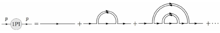
Figure 1: The quark self-energy at the leading in $1/N_{c}$.

Also, by inspecting the diagrams, we see that $\Sigma(p)$ only depends on $p_{-}$. Therefore, we have

$$-i\Sigma(p_{-})=\frac{1}{4\pi}\int\!dk_{+}dk_{-}\,\frac{1}{\left[(k_{-}-p_{-})^{2}\right]_{\lambda}}\,\frac{1}{k_{+}-\Sigma(k_{-})-\frac{m_{q}^{2}}{2k_{-}}+i\varepsilon\,{\rm sgn}(k_{-})}$$ (155)

where ${\rm sgn}(k_{-})\equiv k_{-}/|k_{-}|$ and the notation $[\cdots]_{\lambda}$ is meant to remind us of the IR cutoff on the gluon propagator (150). The $k_{+}$ integral here is log divergent. We choose to remove the divergence by imposing a symmetric cutoff on $k_{+}$ (i.e. $\left|k_{+}\right|\leq\Lambda$) after shifting $k_{+}$ as $k_{+}\longrightarrow k_{+}+\Sigma(k_{-})+m_{q}^{2}/2k_{-}$ to eliminate the terms $-\Sigma(k_{-})-m_{q}^{2}/2k_{-}$ in the denominator. Having done so, we get

$$\Sigma(p_{-})=\frac{{\rm sgn}(p_{-})}{2\lambda}-\frac{1}{2p_{-}}\>.$$ (156)

B.3 The Quark-Antiquark ‘Scattering’ Matrix

Consider the diagrams in figure 2. Here, we are not trying to calculate a scattering amplitude (quarks can never be put on-shell anyway)—rather, since such diagrams will often appear as part of larger diagrams, it is convenient to evaluate them once and for all.

At the leading order in $1/N_{c}$, the only way for the quark and antiquark to exchange gluons is in the “ladder” fashion where all gluons just go vertically connecting the quark and antiquark, and no two gluons ever cross. All diagrams of this type have a $\gamma_{-}$ for each quark line, and one color flows in along the upper-left line and flows out along the lower-left line, and another color, independent of the first one, flows in along the lower-right line and flows out along the upper-right line.

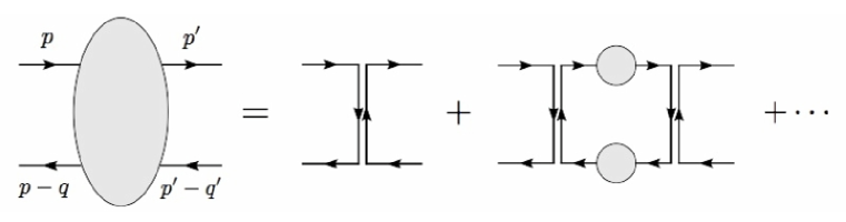
Figure 2: The quark-antiquark ‘scattering’ at the leading order in $1/N_{c}$. A gray circle represents the full quark propagator (154).

Let $T(p,p^{\prime};q)$ be the sum of all such ladder diagrams. (The color indices, the flavor indices, and the factor of $\gamma_{-}\otimes\gamma_{-}$ are suppressed.) Then, we have

$$T(p,p^{\prime};q)=-\frac{i\pi}{N_{c}}\frac{1}{\left[(p_{-}-p^{\prime}_{-})^{2}\right]_{\lambda}}+\frac{i}{4\pi}\int\!dk_{-}\,\frac{1}{\left[(p_{-}-k_{-})^{2}\right]_{\lambda}}\Phi(k_{-},p^{\prime};q)\>,$$ (157)

where

$$\Phi(p_{-},p^{\prime};q)\equiv\int\!dp_{+}\,S(p)\,S(p-q)\,T(p,p^{\prime};q)\>,$$ (158)

and

$$S(p)\equiv\frac{1}{p_{+}-\Sigma(p_{-})-\frac{m_{q}^{2}}{2p_{-}}+i\varepsilon\,{\rm sgn}(p_{-})}\>.$$ (159)

Since by definition $\Phi(p_{-},p^{\prime};q)$ does not depend on $p_{+}$, (157) tells us that $T(p,p^{\prime};q)$ does not depend on $p_{+}$ either. So, the $p_{+}$ integral in (158) converges. For $0<p_{-}/q_{-}<1$ we get

$$\Phi(p_{-},p^{\prime};q)=\frac{2\pi i\,{\rm sgn}(q_{-})\,T(p_{-},p^{\prime};q)}{q_{+}+\Sigma(p_{-}-q_{-})-\Sigma(p_{-})+\frac{m_{q}^{2}}{2(p_{-}-q_{-})}-\frac{m_{q}^{2}}{2p_{-}}+i\varepsilon\,{\rm sgn}(q_{-})}\>,$$ (160)

while for $p_{-}/q_{-}\geq 1$ or $p_{-}/q_{-}\leq 0$ we get

$$\Phi(p_{-},p^{\prime};q)=0\>.$$ (161)

Then, for $0<p_{-}/q_{-}<1$, putting (157) into (160) gives

$$\frac{m_{q}^{2}-1}{\hat{p}(1-\hat{p})}\,\Phi(p_{-},p^{\prime};q)-\hat{{\rm P}}\!\!\int_{0}^{1}\frac{\Phi(q_{-}x,p^{\prime};q)}{(x-\hat{p})^{2}}\,dx$$ (162)

$$= -\frac{4\pi^{2}}{N_{c}\left|q_{-}\right|}\frac{1}{\left[(\hat{p}-\hat{p}^{\prime})^{2}\right]_{\hat{\lambda}}}+(q^{2}+i\varepsilon)\,\Phi(p_{-},p^{\prime};q)\>,$$

where $\hat{p}\equiv p_{-}/q_{-}$, $\hat{p}^{\prime}\equiv p^{\prime}_{-}/q_{-}$, and $\hat{\lambda}\equiv\lambda/\left|q_{-}\right|$. For $0<x<1$, this can be solved in terms of the ’t Hooft wavefunction $\phi_{n}(x)$ satisfying the ’t Hooft equation (2). For $x\leq 0$ or $\geq 0$, we set $\phi_{n}(x)=0$ by definition. Then, we have

$$\Phi(p_{-},p_{-}^{\prime};q)=\frac{4\pi^{2}}{N_{c}\left|q_{-}\right|}\sum_{n}\frac{1}{q^{2}-m_{n}^{2}+i\varepsilon}\,\phi_{n}(\hat{p})\int_{0}^{1}\!\!dx\,\frac{\phi_{n}^{*}(x)}{\left[(x-\hat{p}^{\prime})^{2}\right]_{\hat{\lambda}}}\>,$$ (163)

for all real values of $p_{-}$.

Therefore, we finally get

$$T(p_{-},p^{\prime}_{-};q)=-\frac{i\pi}{N_{c}}\frac{1}{\left[(p_{-}-p^{\prime}_{-})^{2}\right]_{\lambda}}+\frac{4\pi}{N_{c}}\sum_{n}\frac{i}{q^{2}-m_{n}^{2}+i\varepsilon}\frac{\psi_{n}(\hat{p},q_{-})\,\psi_{n}^{*}(\hat{p}^{\prime},q_{-})}{\lambda^{2}}$$ (164)

where

$$\psi_{n}(x,q_{-})\equiv\frac{\lambda}{2|q_{-}|}\int_{0}^{1}\!\!dy\,\frac{\phi_{n}(y)}{[(y-x)^{2}]_{\hat{\lambda}}}\>.$$ (165)

For $0<x<1$, the ’t Hooft equation (2) tells us that $\psi_{n}$ is equal to $\phi_{n}$ up to an $O(\lambda)$ correction:

$$\psi_{n}(x,q_{-})=\left[1-\frac{\lambda}{2\left|q_{-}\right|}\left(m_{n}^{2}-\frac{m_{q}^{2}-1}{x(1-x)}\right)\right]\phi_{n}(x)=\phi_{n}(x)+O(\lambda)\>.$$ (166)

For $x<0$ or $>1$, we can remove the IR cutoff in the integrand in (165), so $\psi_{n}$ can be written as

$$\psi_{n}(x,q_{-})=\frac{\lambda}{2|q_{-}|}\int_{0}^{1}\!\!dy\,\frac{\phi_{n}(y)}{(y-x)^{2}}=O(\lambda)\>.$$ (167)

B.4 Computation of 2-point Correlators

In our gauge $\langle R_{n-}R_{n-}\rangle$ is the easiest one to compute. First, let us define

$$R_{k,\ell}\equiv[(-i\partial_{-})^{k}\overline{\psi}]\gamma_{-}(i\partial_{-})^{\ell}\psi\>,$$ (168)

so that

$$R_{n-}=\sum_{k=0}^{n-1}({}_{n-1}C_{k})^{2}\,R_{n-1-k,k}\>.$$ (169)

Then, in terms of $T(p_{-},p^{\prime}_{-};q)$ calculated above, the correlator can be expressed as in figure 3. The simple quark-loop diagram without a $T$ blob will vanish in the limit of $\lambda\to 0$. The contribution from the one with a $T$ blob is

$$\langle R_{j,k}\,R_{\ell,m}\rangle(q)$$

$$= -N_{c}^{2}\int\!\frac{d^{2}p}{(2\pi)^{2}}\int\!\frac{d^{2}p^{\prime}}{(2\pi)^{2}}\,S(p-q)\,S(P)\,S(p^{\prime}-q)\,S(p^{\prime})$$

$$\quad\times\,p_{-}^{j}\,(p_{-}-q_{-})^{k}\,p_{-}^{\prime m}\,(p^{\prime}_{-}-q_{-})^{\ell}\,T(p_{-},p^{\prime}_{-};q)\,.$$

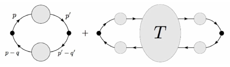
Figure 3: Two-point correlators at the leading order in $1/N_{c}$. The big dots represent the operators $R_{k-}$, $R_{\ell-}$.

Performing $p_{+}$ and $p^{\prime}_{+}$ integrals and taking the $\lambda\to 0$ limit, we obtain

$$\langle R_{j,k}\,R_{\ell,m}\rangle(q)$$ (170)

$$= \frac{N_{c}}{\pi}\sum_{n}\frac{iq_{-}^{j+k+\ell+m+2}}{q^{2}-m_{n}^{2}+i\varepsilon}\left[\int_{0}^{1}\!\!dx\,x^{j}(x-1)^{k}\,\phi_{n}(x)\right]\left[\int_{0}^{1}\!\!dy\,y^{m}(y-1)^{\ell}\,\phi_{n}(y)\right]\>.$$

Now, notice that

$$\sum_{k=0}^{n}({}_{n}C_{k})^{2}x^{n-k}(x-1)^{k}=P_{n}(2x-1)\>,$$ (171)

where $P_{n}$ is the Legendre polynomial. Therefore, we obtain

$$\langle R_{k-}\,R_{\ell-}\rangle(q)$$ (172)

$$= \frac{N_{c}}{\pi}\sum_{n}\frac{iq_{-}^{k+\ell}}{q^{2}-m_{n}^{2}+i\varepsilon}\left[\int_{0}^{1}\!\!dx\,P_{k-1}(2x-1)\,\phi_{n}(x)\right]\!\!\left[\int_{0}^{1}\!\!dy\,P_{\ell-1}(2y-1)\,\phi_{n}(y)\right]$$

Translating this result to the $LL$ case is trivial. Repeating the above steps for $S=\overline{\psi}\psi$ and $P=\overline{\psi}i\gamma_{3}\psi$ to obtain (5) and (6) is also straightforward.

C Details of the Spin-2 Calculation

Due to the special role of the $z$ coordinate in the AdS₃ metric (37) and our choice of gauge (55), it is necessary to treat ‘$3$’ or ‘$z$’ indices separately from ‘$\mu$’ indices. For this purpose, we need to know an explicit expression of the Christoffel symbol for the AdS₃ background $\hat{g}_{AB}=z^{-2}\,\eta_{AB}$:

$$\hat{\Gamma}^{A}_{~{}BC}=-\frac{1}{z}(\delta^{3}_{B}\delta^{A}_{C}+\delta^{3}_{C}\delta^{A}_{B}-\hat{g}^{3A}\hat{g}_{BC})\>.$$ (173)

(Note that $\hat{g}^{3A}\hat{g}_{BC}$ is actually independent of $z$, so the whole $\hat{\Gamma}^{A}_{~{}BC}$ goes as $1/z$.) Using this, we get the following ‘rules’ for $\nabla_{\!\!A}h_{B}^{C}$:

$$\nabla_{\!3}h_{B}^{C} = \partial_{3}h_{B}^{C}$$

$$\nabla_{\!\alpha}h_{\beta}^{\gamma} = \partial_{\alpha}h_{\beta}^{\gamma}-\frac{1}{z}\bigl{(}\delta_{\alpha}^{\gamma}h_{\beta}^{3}+\hat{g}_{\alpha\beta}h^{3\gamma}\bigr{)}$$

$$\nabla_{\!\alpha}h_{\beta}^{3} = \partial_{\alpha}h_{\beta}^{3}-z\bigl{(}h_{\alpha\beta}-\hat{g}_{\alpha\beta}h_{3}^{3}\bigr{)}$$

$$\nabla_{\!\alpha}h_{3}^{3} = \partial_{\alpha}h_{3}^{3}+\frac{2}{z}h_{\alpha}^{3}$$ (174)

To derive (61) from (59), we just use these formulae with the gauge condition $h_{3M}=0$. Next, in (83)-(85), all the terms that are not multiplied by $c$ arise from varying $S_{\rm EH}$ with respect to $h_{3M}$. It is a little more work to get them because we must keep all terms linear in $h_{3M}$ until the end of the calculation. But still it is not so laborious because $S_{\rm EH}$ itself is simple enough.

However, it is much more tedious to derive (66) and especially the $c$-dependent terms in (83)-(85), because $S_{\rm CS}$ contains many more terms with more indices, so just classifying each index into ‘$\mu$’ and ‘$3$’ will give us a large number of terms. Although this is just a matter of algebra, we would like to mention a few things that may help the reader verify those equations.

First, note that, for $g_{AB}=\hat{g}_{AB}+h_{AB}$, we have $\Gamma^{A}_{~{}BC}=\hat{\Gamma}^{A}_{~{}BC}+\delta\Gamma^{A}_{~{}BC}$ where $\delta\Gamma^{A}_{~{}BC}$ consists of $h_{AB}$. Then, correspondingly, we have $\Omega_{\rm CS}=\hat{\Omega}_{\rm CS}+\delta\Omega_{\rm CS}$ where we further split $\delta\Omega_{\rm CS}$ into two parts:

$$\delta\Omega_{\rm CS}=\Omega_{\rm CS}^{(1)}+\Omega_{\rm CS}^{(2)}\>,$$ (175)

where, in terms of the matrix notation introduced in section 3.2.2,

$$\Omega_{\rm CS}^{(1)}\equiv\epsilon^{ABC}\,{\rm Tr}\bigl{[}\delta{\bf\Gamma}_{\!A}\,\partial_{B}\hat{{\bf\Gamma}}_{C}+\hat{{\bf\Gamma}}_{\!A}\,\partial_{B}\delta{\bf\Gamma}_{C}+2\hat{{\bf\Gamma}}_{\!A}\,\hat{{\bf\Gamma}}_{B}\,\delta{\bf\Gamma}_{C}\bigr{]}\>,$$

and

$$\Omega_{\rm CS}^{(2)}\equiv\epsilon^{ABC}\,{\rm Tr}\bigl{[}\delta{\bf\Gamma}_{\!A}\,\partial_{B}\delta{\bf\Gamma}_{C}+2\hat{{\bf\Gamma}}_{\!A}\,\delta{\bf\Gamma}_{B}\,\delta{\bf\Gamma}_{C}\bigr{]}\>.$$ (177)

In the AdS₃ background, $\Omega^{(1)}_{\rm CS}$ is purely a total derivative. This can be seen by first putting it in the following form:

$$\delta\Omega_{\rm CS}^{(1)}=-\epsilon^{ABC}\,\partial_{A}{\rm Tr}\bigl{[}\hat{{\bf\Gamma}}_{B}\,\delta{\bf\Gamma}_{C}\bigr{]}+\epsilon^{ABC}\,{\rm Tr}\bigl{[}\delta{{\bf\Gamma}}_{\!A}\,\hat{{\bf R}}_{BC}\bigr{]}\>.$$ (178)

Then, note that since AdS₃ is maximally symmetric, we have $\hat{R}^{A}_{~{}BCD}=\hat{R}\,(\delta^{A}_{C}\,\hat{g}_{BD}-\delta^{A}_{D}\,\hat{g}_{BC})/6$ where $\hat{R}$ is the scalar curvature, which in turn implies that the second term in the above equation vanishes identically. Therefore, in the AdS₃ background, we have

$$\Omega_{\rm CS}^{(1)}=-\epsilon^{ABC}\,\partial_{A}{\rm Tr}\bigl{[}\hat{{\bf\Gamma}}_{B}\,\delta{\bf\Gamma}_{C}\bigr{]}\>.$$ (179)

So it comes down to evaluating $\Omega_{\rm CS}^{(2)}$. Since it is already quadratic in $\delta\Gamma^{A}_{~{}BC}$, we just need to express $\delta\Gamma^{A}_{~{}BC}$ to first order in $h_{AB}$:

$$\delta\Gamma^{A}_{~{}BC}=\frac{1}{2}(\nabla_{\!B}h^{A}_{C}+\nabla_{\!C}h^{A}_{B}-\nabla^{A}h_{BC})+O(h^{2})$$ (180)

Then, to get the action (66), we apply the rules (174) to the above expression of $\delta\Gamma$ and plug that into $\Omega_{\rm CS}^{(2)}$, which is not so bad because we can use the gauge condition $h_{3A}=0$ from the beginning of the calculation.

What is grueling is to get the $c$-dependent terms in the constraint equations (83)-(85), because we need to keep $h_{3M}$ to linear order until the end of the calculation in order for us to be able to vary $S_{\rm CS}$ with respect to $h_{3M}$. Fortunately, in the above expression (177) of $\Omega_{\rm CS}^{(2)}$, we have no more than one $\nabla$ acting on $h_{AB}$, so we can still use the rules (174). This is a lengthy but straightforward calculation. A better way is to first combine the two terms in (177) to get

$$\Omega_{\rm CS}^{(2)}\equiv\epsilon^{ABC}\,{\rm Tr}\bigl{[}\delta{\bf\Gamma}_{\!A}\nabla_{\!B}\delta{\bf\Gamma}_{C}\bigr{]}\>.$$ (181)

This simple appearance is actually deceiving, because now we have two $\nabla$’s acting on $h_{AB}$, so we need extend the rules (174) to the case with two covariant derivatives, which will be many more rules than the one-derivative case. So, we should use the commutation relation (62) to eliminate $\nabla$’s as much as possible. Below we sketch how the calculation proceeds when one does it this way.

First, using (180), we can write (181) explicitly in terms of $h_{AB}$:

$$\Omega_{\rm CS}^{(2)}=\frac{1}{4}\epsilon^{ABC}(\nabla_{\!\!A}h^{DE})\,\nabla_{\!B}\nabla_{\!C}h_{DE}+\frac{1}{2}\epsilon^{ABC}(\nabla^{E}h^{D}_{A})\,\nabla_{\!B}(\nabla_{\!D}h_{CE}-\nabla_{\!E}h_{CD})\>.$$ (182)

Then, varying $\Omega_{\rm CS}^{(2)}$ with respect to $h_{AB}$ gives

$$\frac{\delta}{\delta h_{DE}}\int\!d^{3}x\,\Omega_{\rm CS}^{(2)}$$ (183)

$$= -\frac{1}{2}\left[\frac{1}{2}\epsilon^{ABC}\nabla_{\!\!A}\nabla_{\!B}\nabla_{\!C}h_{DE}+\epsilon^{EBC}\nabla_{\!\!A}\nabla_{\!B}(\nabla^{D}h^{A}_{C}-\nabla^{A}h^{D}_{C})+(D\leftrightarrow E)\right]$$

where $(D\leftrightarrow E)$ represents the whole expression before it with $D$ and $E$ swapped. Now, the three $\nabla$’s in the first term above can be immediately reduced to one $\nabla$ using the commutator (62) since they are already anti-symmetrized due to the $\epsilon$ tensor. In a maximally symmetric space such as AdS₃, it simplifies down to

$$\epsilon^{ABC}\nabla_{\!\!A}\nabla_{\!B}\nabla_{\!C}h_{DE}=-\frac{\hat{R}}{6}\left[\epsilon^{DAB}\nabla_{\!\!A}h^{E}_{B}+(D\leftrightarrow E)\right]\>.$$ (184)

As for $\epsilon^{EBC}\nabla_{\!\!A}\nabla_{\!B}\nabla^{D}h^{A}_{C}$, we can simplify it (in a maximally symmetric space) as

$$\epsilon^{EBC}\nabla_{\!\!A}\nabla_{\!B}\nabla^{D}h^{A}_{C}+(D\leftrightarrow E)=\epsilon^{EBC}\left(\nabla^{D}\nabla_{\!B}\nabla_{\!\!A}h^{A}_{C}+\frac{2\hat{R}}{3}\,\nabla_{\!B}h^{D}_{C}\right)+(D\leftrightarrow E)\>.$$ (185)

This is in fact better than the original expression; first, the $\hat{R}$ term can be combined with (184). Second, note that the $\nabla_{\!B}$ in the first term can be replaced with $\partial_{B}$. Then, we write out the $\nabla^{D}$ explicitly in terms of $\partial$ and $\hat{\Gamma}$. Now we have only one $\nabla$ left, which in our $h_{3A}=0$ gauge gives

$$\nabla_{\!\!A}h^{A}_{C}=\partial_{A}h^{A}_{C}+\frac{1}{z}\delta^{3}_{C}h\>.$$ (186)

We then obtain

$$\epsilon^{EBC}\nabla^{D}\nabla_{\!B}\nabla_{\!\!A}h^{A}_{C}+(D\leftrightarrow E)$$ (187)

$$= \epsilon^{DAB}\hat{g}^{EF}\biggl{[}\partial_{F}\partial_{A}\partial_{C}h^{C}_{B}+\frac{1}{z}\delta^{3}_{A}\partial_{F}\partial_{C}h^{C}_{B}+\frac{1}{z}\delta^{3}_{B}\partial_{F}\partial_{A}h+\frac{1}{z}\delta^{3}_{B}\partial_{A}\partial_{C}h^{C}_{F}$$

$$\hskip 50.00008pt-2z\,\hat{g}_{3F}\,\partial_{A}\partial_{C}h^{C}_{B}-2\hat{g}_{3F}\,\delta^{3}_{B}\partial_{A}h\biggr{]}+(D\leftrightarrow E)\>.$$

Next, going back to (183), we have

$$\epsilon^{EBC}\nabla_{\!\!A}\nabla_{\!B}\nabla^{A}h^{D}_{C}+(D\leftrightarrow E)=\epsilon^{EBC}\left(\nabla_{\!B}\nabla^{2}h^{D}_{C}+\frac{\hat{R}}{6}\nabla_{\!B}h^{D}_{C}\right)+(D\leftrightarrow E)\>.$$ (188)

Again, the $\hat{R}$ term can be combined with (184). The three-$\nabla$ term is not so bad since two of them are contracted, and exploiting the anti-symmetry between $B$ and $C$, we can simplify it to

$$\epsilon^{EBC}\nabla_{\!B}\nabla^{2}h^{D}_{C}+(D\leftrightarrow E)=\epsilon^{EBC}\left(\partial_{B}-\frac{1}{z}\delta^{3}_{B}\right)\!\nabla^{2}h^{D}_{C}\>.$$ (189)

This $\nabla^{2}$ term must be computed by brute force, but this is the only one. It becomes

$$\nabla^{2}h^{D}_{C}=\hat{g}^{AF}\partial_{A}\partial_{F}h^{D}_{C}+z\partial_{3}h^{D}_{C}+\frac{2}{z}\delta^{3}_{C}\partial_{A}h^{AD}-2z\delta^{D}_{3}\partial_{A}h^{A}_{C}+2h^{D}_{C}-2\delta^{D}_{3}\delta^{3}_{C}h\>.$$ (190)

Putting all the pieces together (with $\hat{R}=6$ for AdS₃), we obtain

$$-\frac{\delta}{\delta h_{DE}}\int\!d^{3}x\,\Omega_{\rm CS}^{(2)}$$ (191)

$$= \frac{1}{2}\epsilon^{DAB}\biggl{[}2\nabla_{\!\!A}h^{E}_{B}+\hat{g}^{EF}\biggl{(}\partial_{F}\partial_{A}\partial_{C}h^{C}_{B}+\frac{1}{z}\delta^{3}_{B}\partial_{F}\partial_{A}h+\frac{1}{z}\delta^{3}_{A}\partial_{F}\partial_{C}h^{C}_{B}\biggr{)}$$

$$\hskip 30.00005pt-\hat{g}^{CF}\biggl{(}\partial_{C}\partial_{F}\partial_{A}h^{E}_{B}+\frac{1}{z}\delta^{3}_{A}\partial_{C}\partial_{F}h^{E}_{B}\biggr{)}-z\partial_{A}\partial_{3}h^{E}_{B}-\frac{1}{z}\delta^{3}_{B}\partial_{A}\partial_{C}h^{CE}$$

$$\hskip 30.00005pt-2\partial_{A}h^{E}_{B}+\frac{2}{z}\delta^{3}_{A}h^{E}_{B}\biggr{]}+(D\leftrightarrow E)\>.$$

References

- [1] J. M. Maldacena, “The large N limit of superconformal field theories and supergravity,” Adv. Theor. Math. Phys. 2, 231 (1998) [Int. J. Theor. Phys. 38, 1113 (1999)] [arXiv:hep-th/9711200]; S. S. Gubser, I. R. Klebanov and A. M. Polyakov, “Gauge theory correlators from non-critical string theory,” Phys. Lett. B 428, 105 (1998) [arXiv:hep-th/9802109]; E. Witten, “Anti-de Sitter space and holography,” Adv. Theor. Math. Phys. 2, 253 (1998) [arXiv:hep-th/9802150].
- [2] D. E. Berenstein, J. M. Maldacena and H. S. Nastase, “Strings in flat space and pp waves from N = 4 super Yang Mills,” JHEP 0204, 013 (2002) [arXiv:hep-th/0202021].
- [3] J. Erlich, E. Katz, D. T. Son and M. A. Stephanov, “QCD and a holographic model of hadrons,” Phys. Rev. Lett. 95, 261602 (2005) [arXiv:hep-ph/0501128].
- [4] E. Katz, A. Lewandowski and M. D. Schwartz, “Tensor mesons in AdS/QCD,” Phys. Rev. D 74, 086004 (2006) [arXiv:hep-ph/0510388].
- [5] E. Katz and M. D. Schwartz, “An eta primer: Solving the U(1) problem with AdS/QCD,” arXiv:0705.0534 [hep-ph].
- [6] A. Karch, E. Katz, D. T. Son and M. A. Stephanov, “Linear confinement and AdS/QCD,” Phys. Rev. D 74, 015005 (2006) [arXiv:hep-ph/0602229].
- [7] G. ’t Hooft, “A Two-Dimensional Model For Mesons,” Nucl. Phys. B 75, 461 (1974).
- [8] C. G. Callan, N. Coote and D. J. Gross, “Two-Dimensional Yang-Mills Theory: A Model Of Quark Confinement,” Phys. Rev. D 13, 1649 (1976).
- [9] R. C. Brower, W. L. Spence and J. H. Weis, “Bound States And Asymptotic Limits For QCD In Two-Dimensions,” Phys. Rev. D 19, 3024 (1979).
- [10] S. J. Brodsky and G. F. de Teramond, arXiv:0709.2072 [hep-ph].
- [11] R. Narayanan and H. Neuberger, “The quark mass dependence of the pion mass at infinite N,” Phys. Lett. B 616, 76 (2005) [arXiv:hep-lat/0503033].
- [12] S. R. Coleman, “There are no Goldstone bosons in two-dimensions,” Commun. Math. Phys. 31, 259 (1973); N. D. Mermin and H. Wagner, “Absence of ferromagnetism or antiferromagnetism in one-dimensional or two-dimensional isotropic Heisenberg models,” Phys. Rev. Lett. 17, 1133 (1966).
- [13] E. Witten, “Chiral Symmetry, The 1/N Expansion, And The SU(N) Thirring Model,” Nucl. Phys. B 145, 110 (1978).
- [14] S. Deser, R. Jackiw and S. Templeton, “Three-Dimensional Massive Gauge Theories,” Phys. Rev. Lett. 48 (1982) 975.
- [15] G. Guralnik, A. Iorio, R. Jackiw and S. Y. Pi, “Dimensionally reduced gravitational Chern-Simons term and its kink,” Annals Phys. 308, 222 (2003) [arXiv:hep-th/0305117].
- [16] J. Polchinski and M. J. Strassler, “Deep inelastic scattering and gauge/string duality,” JHEP 0305, 012 (2003) [arXiv:hep-th/0209211].