Spectra of graph neighborhoods and scattering

Abstract.

Let $(G_{\varepsilon})_{\varepsilon>0}$ be a family of ’$\varepsilon$-thin’ Riemannian manifolds modeled on a finite metric graph $G$, for example, the $\varepsilon$-neighborhood of an embedding of $G$ in some Euclidean space with straight edges. We study the asymptotic behavior of the spectrum of the Laplace-Beltrami operator on $G_{\varepsilon}$ as $\varepsilon\to 0$, for various boundary conditions. We obtain complete asymptotic expansions for the $k$th eigenvalue and the eigenfunctions, uniformly for $k\leq C\varepsilon^{-1}$, in terms of scattering data on a non-compact limit space. We then use this to determine the quantum graph which is to be regarded as the limit object, in a spectral sense, of the family $(G_{\varepsilon})$.

Our method is a direct construction of approximate eigenfunctions from the scattering and graph data, and use of a priori estimates to show that all eigenfunctions are obtained in this way.

1. Introduction

Consider a graph $G$ with a finite number of vertices and edges embedded in $\mathbb{R}^{n}$ with straight edges. For $\varepsilon>0$ let $G_{\varepsilon}$ be the set of points of distance at most $\varepsilon$ from $G$. For small $\varepsilon$, $G_{\varepsilon}$ ’looks almost like’ $G$; in other words, the one-dimensional object $G$ should be considered as a good model for $G_{\varepsilon}$, and so one expects many physical and analytical properties of $G_{\varepsilon}$ to be understandable, in an approximate sense, by corresponding properties of $G$. The property we analyze in this light here is the spectrum of the Laplacian, under various boundary conditions. For motivation from physics, see for example [13].

This problem has received some attention in the last decade. The case of Neumann boundary conditions was analyzed at various levels of generality in [4], [6], [15], [21], [5], where it was shown that for each $k\in\mathbb{N}$ the $k$th eigenvalue of the Neumann Laplacian on $G_{\varepsilon}$ converges, as $\varepsilon\to 0$, to the $k$th eigenvalue of the second derivative operator on the union of the edges of $G$, where at the vertices so-called Kirchhoff boundary conditions are imposed. The question of what the corresponding limiting behavior is for other, for example Dirichlet, boundary conditions was characterized as ’very difficult’ in [5] and remained open until some partial progress was made recently, see Section 1.4.

In this paper we solve this problem for a general mixed boundary problem, where we impose Dirichlet boundary conditions on one part of the boundary and Neumann conditions on the rest. Other boundary conditions, for example Robin, are also possible. Instead of the setting of an embedded graph described above, we consider the more general, and mathematically more natural, situation of a shrinking family of Riemannian manifolds modeled on the graph: We now consider $G$ as an abstract metric graph, that is, for each edge $e$ a positive number $l_{e}$ (to be thought of as half the edge length) is given. In addition, we have geometric data: For each edge $e$ an $(n-1)$-dimensional Riemannian manifold $Y_{e}$, and for each edge $v$ an $n$-dimensional Riemannian manifold $X_{v}$; all these manifolds are compact and may have a piecewise smooth boundary; also, for each edge $e$ incident to a vertex $v$ (denoted $e\sim v$), we are given an identification (gluing map) of $Y_{e}$ with a subset of the boundary of $X_{v}$, without overlaps. Then $G_{\varepsilon}$ is defined by gluing cylinders of length $2l_{e}$ and cross section $\varepsilon Y_{e}$ (the factor denotes a rescaling of the metric) to $\varepsilon X_{v}$ for all pairs $e\sim v$. Also given are subsets D and N of the boundaries of each $X_{v}$ and $Y_{e}$, which yield corresponding subsets of $G_{\varepsilon}$ (or, for Robin conditions, similar data). We investigate the Laplace-Beltrami operator on $G_{\varepsilon}$, where Dirichlet boundary conditions are imposed on D and Neumann conditions on N. We suppose sufficient regularity of the boundary and the D/N decomposition so that this problem has discrete spectrum.

Besides the $\varepsilon$-neighborhoods mentioned before this manifold setting includes the case of the boundary of the $\varepsilon$-neighborhood of $G$ (in this case, $G_{\varepsilon}$ itself has no boundary). Our results imply the following theorem.

Theorem 1.

Let $\mu_{1}(\varepsilon)\leq\mu_{2}(\varepsilon)\leq\dotsc$ be the eigenvalues of the Laplacian on $G_{\varepsilon}$, with the given boundary conditions, repeated according to their multiplicity.

For each edge $e$, let $\nu_{e}$ be the smallest eigenvalue of $-\Delta$ on $Y_{e}$, with the given boundary conditions, and let $\nu=\min_{e}\nu_{e}$.

There are numbers $D\in\mathbb{N}_{0}$, $0<\tau_{1}\leq\tau_{2}\leq\dotsc\leq\tau_{D}\leq\nu$ and $0\leq b_{1}\leq b_{2}\leq\dots\to\infty$ so that for $\varepsilon\to 0$

(1) $$\mu_{k}(\varepsilon) =\varepsilon^{-2}\tau_{k}+O(e^{-c/\varepsilon}), k=1,\dots,D$$

(2) $$\mu_{k}(\varepsilon) =\varepsilon^{-2}\nu+b_{k-D}+O(\varepsilon), k>D$$

In fact, we obtain much more precise information: complete asymptotics up to errors of the form $O(e^{-c/\varepsilon})$ also in the case $k>D$, uniform estimates not only for fixed $k$ but also for $k$ on the order of $\varepsilon^{-1}$ as well as detailed information on the eigenfunctions, see the theorems below.

For Theorem 1 to be meaningful it is essential to identify the numbers $\tau_{k}$ and $b_{k}$ in terms of the given data. We do this in two steps: First, we give general formulas identifying these numbers in terms of scattering data of an associated non-compact $n$-dimensional limiting problem. Second, we analyze how this scattering data can be obtained from the given data. It turns out that in this second step the situation of general boundary conditions carries some essential new features compared to Neumann boundary conditions: while in this case one has $D=0$ and the $b_{k}$ are determined by the graph and the edge lengths alone (that is, independent of the manifolds $X_{v}$, $Y_{e}$), in general $D>0$ and the $\tau_{k}$ and $b_{k}$ depend also on transcendental analytic information involving the manifolds $X_{v}$ and $Y_{e}$: The $\tau_{k}$ are $L^{2}$-eigenvalues in the afore-mentioned limit problem, and the $b_{k}$ are eigenvalues of a quantum graph whose vertex boundary conditions involve the scattering matrix of that limit problem, see Theorems 2 and 3.

1.1. Main results

We now state our results more precisely. Because of the divergence in (1), (2) it is more convenient, and for a proper understanding it turns out to be essential, to rescale the problem: We multiply all lengths by $\varepsilon^{-1}$. We denote

$$N:=\varepsilon^{-1},\quad X^{N}_{G}:=\varepsilon^{-1}G_{\varepsilon}$$

This rescales the eigenvalues by the factor $\varepsilon^{2}$. In $X^{N}_{G}$, the vertex manifolds and the cross sections of the edges are independent of $N$ while the lengths of the edges are $2Nl_{e}$, and we are interested in the limit $N\to\infty$. Central to the analysis is the limit object, to be thought of as $\lim_{N\to\infty}X^{N}_{G}$,

(3) $$X^{\infty}:=\bigcup_{v}X_{v}^{\infty}\quad\text{ (disjoint union)}$$

where the ’star’ $X^{\infty}_{v}$ of a vertex $v$ of $G$ is obtained by attaching a half infinite cylinder $[0,\infty)\times Y_{e}$ to the vertex manifold $X_{v}$, for each edge $e$ incident to $v$, see Figure 1. Denote by $Y$ the cross-section for $X^{\infty}$, i.e. the disjoint union of the $Y_{e}$, each one appearing twice (once for each endpoint). The graph structure is encoded by a map $\sigma:Y\to Y$ which toggles the two copies of $Y_{e}$ for each edge $e$. See Section 2 for precise definitions.

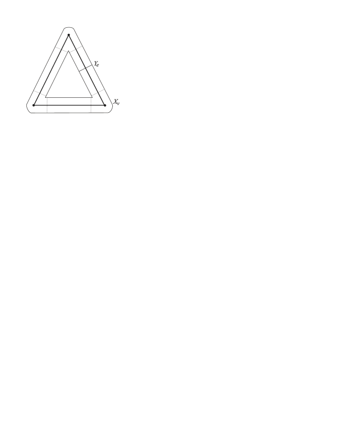
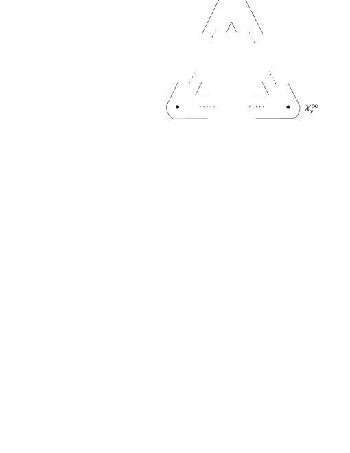
Figure 1. The setup: $X^{N}_{G}$ and $X^{\infty}$

Since $X^{\infty}$ is a non-compact space, the spectrum of the Laplacian $-\Delta_{X^{\infty}}$ (with corresponding boundary conditions) is no longer discrete. Its spectral theory is obtained via scattering theory, that is, one considers it as compact perturbation of $[0,\infty)\times Y$, the disjoint union of the edge cylinders. Let $\nu<\nu_{1}$ be the smallest and second smallest eigenvalue of the Laplacian of $Y$ and let $V$ be the eigenspace corresponding to $\nu$. The absolutely continuous spectrum of $-\Delta_{X^{\infty}}$ is $[\nu,\infty)$. To each $\lambda=\nu+\alpha^{2}\in[\nu,\nu_{1})$ is associated the scattering matrix $S(\alpha)$, a linear map $V\to V$ depending holomorphically on $\alpha$, and to each $\varphi\in V$ a scattering solution (generalized eigenfunction) $E_{\alpha,\varphi}$. These are the main objects of scattering theory. In addition, $-\Delta_{X^{\infty}}$ may have discrete spectrum ($L^{2}$-eigenvalues).

We also have linear maps $L,\sigma:V\to V$ where $L$ encodes the edge lengths (it equals $l_{e}{\rm Id}$ on the subspace of $V$ corresponding to the edge $e$) and $\sigma$ is induced by the graph structure map above. The maps $\sigma$ and $S(0)$ are involutions on $V$, so they have only the eigenvalues $\pm 1$.

We need the following data derived from the spectral data of $-\Delta_{X^{\infty}}$:

• The $L^{2}$-eigenvalues $\tau_{1}^{\prime}<\tau_{2}^{\prime}<\dotsc<\tau_{d}^{\prime}<\nu_{1}$ of $-\Delta_{X^{\infty}}$, with eigenspaces ${\mathcal{E}}_{1},\dotsc,{\mathcal{E}}_{d}\subset L^{2}(X^{\infty})$;

• the space ${\mathcal{P}}_{0}:=\operatorname{Ker}({\rm Id}-\sigma)\cap\operatorname{Ker}({\rm Id}-S(0))\subset V$.

• the spaces ${\mathcal{P}}_{z}:=\operatorname{Ker}({\rm Id}-e^{iz2L}\sigma S(0))\subset V$ for $z>0$. This is non-zero for a discrete set

  (4) $$0<z_{1}<z_{2}<\dotsc\quad\text{the zeroes of }f(z)=\det({\rm Id}-e^{iz2L}\sigma S(0))$$

• for each $i\in\mathbb{N}$, pairwise different holomorphic functions $Z_{i}^{\rho}(\alpha)$, $\rho=1,\dots,r_{i}$ with $r_{i}\in\mathbb{N}$, defined on $\mathbb{C}\setminus\{\alpha\in\mathbb{R}:\,|\alpha|\geq\nu_{1}\}$ and with

  (5) $$Z_{i}^{\rho}(0)=z_{i}$$

  for each $\rho$, and holomorphically varying subspaces ${\mathcal{P}}_{i}^{\rho}\subset V$ with $\bigoplus_{\rho=1}^{r_{i}}{\mathcal{P}}_{i}^{\rho}(0)={\mathcal{P}}_{z_{i}}$.

The $Z_{i}^{\rho}$ and ${\mathcal{P}}_{i}^{\rho}$ arise from a bifurcation analysis of $\operatorname{Ker}({\rm Id}-e^{iz2L}\sigma S(\alpha))$, see Theorem 15.

Theorem 2 (Main Theorem).

Denote by $-\Delta_{X_{G}^{N}}$ the Laplace-Beltrami operator on $X^{N}_{G}$, with the given boundary conditions. For any $\lambda_{\rm max}<\nu_{1}$ there are $c,N_{0}>0$ such that for $N>N_{0}$ the spectrum of $-\Delta_{X_{G}^{N}}$ in $[0,\lambda_{\rm max}]$ consists of (counting multiplicities)

1. $\dim{\mathcal{E}}_{p}$ many eigenvalues of the form $\tau_{p}^{\prime}+O(e^{-cN})$, for $p=1,\dotsc,d$,

2. $\dim{\mathcal{P}}_{0}$ many eigenvalues of the form $\nu+O(e^{-cN})$,

3. $\dim{\mathcal{P}}_{i}^{\rho}$ many eigenvalues of the form

   (6) $$\nu+\beta^{2}\text{ with }\beta=\frac{1}{N}Z_{i}^{\rho}(\frac{1}{N})+O(e^{-cN})$$

   for each $i\in\mathbb{N}$ and $\rho=1,\dots,r_{i}$ for which $\nu+\beta^{2}\leq\lambda_{\rm max}$.

The constants $c,N_{0}$ and the constants in the big $O$ only depend on the spectral data of $\Delta_{X^{\infty}}$. In particular, the asymptotics are uniform for eigenvalues $\leq\lambda_{\rm max}$.

In terms of $\varepsilon=N^{-1}$ (6) gives an eigenvalue $\mu=\nu+\varepsilon^{2}z_{i}^{2}+O(\varepsilon^{3})$ by (5), so this implies Theorem 1: take $D=\sum_{p=1}^{d^{\prime}}\dim{\mathcal{E}}_{p}$ with $d^{\prime}=\max\{p:\tau_{p}^{\prime}\leq\nu\}$; the $\tau_{k}$ are the $\tau_{p}^{\prime}$ repeated $\dim{\mathcal{E}}_{p}$ times; and the $b_{k}$ are $0$ repeated $\dim{\mathcal{P}}_{0}$ times, and the numbers $z_{i}^{2}$ repeated $\dim{\mathcal{P}}_{i}$ many times. The $\tau_{p}$ with $p>d^{\prime}$ are invisible in Theorem 1 since there $k$ is fixed as $\varepsilon\to 0$.

Theorem 2 also describes eigenvalue $\mu_{k}$ with $k\to\infty$ as $\varepsilon\to 0$. We determine the permitted range of $k$. From $\mu_{k}=\nu+\varepsilon^{2}z_{i}^{2}+O(\varepsilon^{3})\leq\lambda_{\rm max}$ one obtains $\varepsilon z_{i}<\sqrt{\lambda_{\rm max}-\nu}+O(\varepsilon)$, and the Weyl asymptotics for the $z_{i}$, see Proposition 13, show that this is equivalent to

(7) $$k\leq\varepsilon^{-1}\frac{\sum_{e}l_{e}}{\pi}\sqrt{\lambda_{\rm max}-\nu}+O(1).$$

See Theorem 16 for a more explicit description of eigenvalues with $\beta$ close to some $\beta_{0}>0$.

We can also describe the eigenfunctions in terms of the scattering solutions and of the eigenfunctions in ${\mathcal{E}}_{p}$, with exponentially small errors, see Theorems 21, 22 and 24 and Corollary 23 for precise statements.

The restriction $\lambda_{\rm max}<\nu_{1}$ is made to keep the exposition at a reasonable length. Our methods are such that a generalization to higher eigenvalues, taking into account several thresholds, should be fairly straightforward.

To identify the numbers $b_{k}$ in Theorem 1 in terms of the data, we recall that a quantum graph is given by a metric graph ($G$ with the edge lengths $2l_{e}$) together with a self-adjoint realization of the operator $-d^{2}/d\xi^{2}$ acting on functions defined on the disjoint union of the edges, where $\xi$ is a variable along each edge, measuring length; such a self-adjoint extension is given by boundary conditions at the vertices. We state the boundary conditions obtained in our setting. Denote by

$${\mathcal{N}}_{e}:=\ker(\Delta_{Y_{e}}+\nu)$$

the eigenspace for $\nu$ of the Laplacian on the cross section for an edge $e$. For each vertex $v$ let $V_{v}=\bigoplus_{e\sim v}{\mathcal{N}}_{e}$, then clearly $V=\bigoplus_{v}V_{v}$ corresponding to the decomposition (3). Also, the scattering matrix $S(\alpha)$ is the direct sum of scattering matrices $S_{v}(\alpha):V_{v}\to V_{v}$. For each vertex $v$, $S_{v}(0)$ is an involution on $V_{v}$. Denote by $u_{e}$ the restriction of a function on $G$ to the edge $e$, and by $\partial_{n}u_{e}(v)$ its inward normal derivative at the endpoint $v$ of $e$.

Theorem 3.

The numbers $b_{k}$ in (2) are the eigenvalues of the operator $-d^{2}/d\xi^{2}$ on the metric graph $G$ with edge lengths $2l_{e}$, defined on the space of functions $u$ which on each edge $e$ are smooth and take values in ${\mathcal{N}}_{e}$ and which at each vertex $v$ satisfy the boundary conditions

(8) $$(u_{e}(v))_{e\sim v} \in(+1)-\text{eigenspace of }S_{v}(0)$$

(9) $$(\partial_{n}u_{e}(v))_{e\sim v} \in(-1)-\text{eigenspace of }S_{v}(0).$$

Remarks.

1. If, for some edge $e$, the lowest eigenvalue on $Y_{e}$ is bigger than $\nu$, then ${\mathcal{N}}_{e}=\{0\}$, so $u_{e}$ has to be identically zero, which means that the edge $e$ may be omitted from $G$. In other words, only the ’thickest’ edges contribute substantially to the eigenvalue $\mu_{k}(\varepsilon)$, for small $\varepsilon$.

2. If $Y_{e}$ is connected then ${\mathcal{N}}_{e}$ is one-dimensional, so it can be identified with $\mathbb{C}$. But in general there is no canonical eigenfunction, so this identification is not canonical. However, if all $Y_{e}$ are the same connected Riemannian manifold (for example, in the case of an $\varepsilon$-neighborhood of an embedded graph, where they are balls) one may choose the same basis element in each ${\mathcal{N}}_{e}$, so one may think of $u$ as a complex valued function and $V_{v}\cong\mathbb{C}^{\deg(v)}$ where $\deg(v)$ is the degree of $v$.

3. Two special cases deserve to be mentioned:

   • Dirichlet conditions at the vertex $v$ correspond to $S_{v}(0)=-{\rm Id}$. In particular, if $S(0)=-{\rm Id}$ then the limit quantum graph is completely decoupled (Dirichlet boundary value problem on each edge separately, without interaction between edges).

   • If all ${\mathcal{N}}_{e}$ are identified with $\mathbb{C}$ and $S_{v}(0)$ has $(+1)$-eigenspace spanned by the vector $(1,1,\dots,1)$ then (8) says that $u$ is continuous at $v$ and (9) (which is equivalent to $(\partial_{n}u_{e}(v))_{e\sim v}\perp(1,\dots,1)$) that the sum of normal derivatives of the $u_{e}$ vanishes at $v$. This is often called the ’Kirchhoff boundary condition’.

4. Theorems 1 and 3 show clearly the two ingredients that determine the leading behavior of eigenvalues:

   • The determination of $S(0)$ and of the $L^{2}$-eigenvalues $\tau_{k}$ is a transcendental problem, depending on the vertex and edge manifolds (for example, in the situation of the $\varepsilon$-neighborhood of an embedding, the angle at which edges meet).

   • Given $S(0)$, the $b_{k}$ are determined solely by the combinatorics of the underlying metric graph.

   In the special case of pure Neumann boundary conditions and of Dirichlet conditions with ’small’ vertex manifolds the leading behavior of eigenvalues is determined by the metric graph alone, see Theorem 25. That is, it is independent of the manifolds $X_{v},Y_{e}$. This may be seen as reason why the general case is harder to analyze. These cases were known previously, see [15], [21], [5] and [20].

   It is known that ’usually’ (for example in the embedded situation) there are $L^{2}$-eigenvalues $\tau<\nu$, so they can not be neglected. See, for example, [22], [2].

Using Theorem 3 one can show that for generic geometric data (for example, an open dense set of Riemannian metrics on the vertex and edge manifolds) one has $S(0)=-{\rm Id}$, that is decoupled Dirichlet conditions for the quantum graph at all vertices. This will be pursued in a separate paper.

1.2. Outline of the proof of the Main Theorem

We now give an outline of the proof of Theorem 2, where for simplicity we assume that all $l_{e}=1$: Let $x$ be a coordinate on the cylindrical part of $X^{\infty}$ and of $X^{N}_{G}$, measuring length along the cylinder axis (going from $0$ to $N$ from both ends of the cylinder axis).

The proof consists of two steps: First, we use the spectral data on $X^{\infty}$ to construct approximate eigenfunctions on $X^{N}_{G}$ for large $N$ and conclude the existence of eigenvalues and eigenfunctions as claimed. Second, we show that all eigenfunctions on $X^{N}_{G}$ are obtained this way.

For clarity we assume in this outline that all multiplicities (i.e. dimensions of ${\mathcal{E}}_{p}$ and ${\mathcal{P}}_{z}$) are equal to one and that $\tau_{p}<\nu$ for all $p$ (no embedded eigenvalues). We will call a quantity ’very small’ if it is exponentially small as $N\to\infty$, i.e. $O(e^{-cN})$ for some $c>0$.

Throughout, eigenvalues on $X^{N}_{G}$ will be denoted $\mu$, with $\mu=\nu+\beta^{2}$ if $\mu\geq\nu$, and spectral values for $X^{\infty}$ by $\lambda$, with $\lambda=\nu+\alpha^{2}$ if $\lambda\geq\nu$.

Case I: Eigenvalues $\mu<\nu-c$: Here, everything is quite straightforward.

• First step: If $U$ is an eigenfunction on $X^{\infty}$ with eigenvalue $\lambda=\tau_{p}<\nu$ then $U$ decreases exponentially in $x$. So if we simply cut off $U$ smoothly near $x=N$, making it zero near $x=N$, then we get a function on $X^{N}_{G}$ which satisfies the eigenfunction equation up to a very small error. A simple spectral approximation lemma, Lemma 7, shows that $-\Delta_{X_{G}^{N}}$ has an eigenvalue very close to $\lambda$. A spectral gap argument gives a similar approximation for the eigenfunction.

• Second step: This procedure can be reversed: If $u$ is an eigenfunction on $X^{N}_{G}$ with eigenvalue $\mu<\nu-c$ then it decreases exponentially in $x$, so cutting it off near $x=N$ yields a function on $X^{\infty}$ which satisfies the eigenfunction equation up to a very small error. Since $-\Delta_{X^{\infty}}$ has purely discrete spectrum near $\mu$, it follows by the spectral approximation lemma that it has an eigenvalue very close to $\mu$. Therefore, there can be no eigenfunctions on $X^{N}_{G}$ in addition to those constructed in the first step.

Case II: Eigenvalues $\mu\in(\nu+e^{-cN},\lambda_{\rm max}]$: A basic observation is that any eigenfunction $u$ on $X^{N}_{G}$ or generalized eigenfunction on $X^{\infty}$ with eigenvalue $\lambda\in(\nu,\nu_{1})$ can on the cylindrical part be written as $\Pi u+\Pi^{\perp}u$, where $\Pi u$, called the leading part, is the first mode in the $Y$-direction. $\Pi u$ is of the form

(10) $$\Pi u=e^{-i\alpha x}\varphi+e^{i\alpha x}\psi,\quad\varphi,\psi\in V,\quad\alpha:=\sqrt{\lambda-\nu}$$

and $\Pi^{\perp}u$ is exponentially decreasing in $x$.

• First step: The scattering solutions $E=E_{\alpha,\varphi}$ have leading part of the form (10) with $\psi=S(\alpha)\varphi$. Since $\Pi E$ is not decaying as $x\to\infty$, we should only cut off $\Pi^{\perp}E$ near $x=N$, in order to obtain a small error term when constructing an approximate eigenfunction on $X^{N}_{G}$ from $E$. Therefore, we must require $\Pi E_{\alpha,\varphi}$ to satisfy matching conditions at $x=N$ that make it a smooth function on the cylindrical part of $X^{N}_{G}$. A short calculation shows that this is equivalent to the equation

  (11) $$M(\alpha,\varphi)=0,\quad\text{where }M(\alpha,\varphi):=\left[{\rm Id}-e^{i\alpha N2L}\sigma S(\alpha)\right]\varphi\in V.$$

  Perturbation theory gives functions $Z_{i}^{\rho}$ and spaces ${\mathcal{P}}_{i}^{\rho}$ so that the solutions of this equation are $\alpha=\frac{1}{N}Z_{i}^{\rho}(\frac{1}{N})$ and $\varphi\in{\mathcal{P}}_{i}^{\rho}(\frac{1}{N})$. So for these $\alpha,\varphi$ the function obtained from $E=E_{\alpha,\varphi}$ by cutting of $\Pi^{\perp}E$ near $x=N$ satisfies the eigenvalue equation on $X^{N}_{G}$ with a very small error. Therefore, one gets eigenvalues as in (6).

• Second step: It remains to show that for large $N$ all eigenvalues $\mu\in(\nu+e^{-cN},\lambda_{\rm max}]$ on $X^{N}_{G}$ are obtained in this way. This is the theoretically most demanding part of the proof. Let $u$ be an eigenfunction of $-\Delta_{X_{G}^{N}}$ with eigenvalue $\mu=\nu+\beta^{2},\beta>e^{-cN/2}$. An argument directly analogous to the case $\mu<\nu$ won’t work since it only yields that $-\Delta_{X^{\infty}}$ has nonempty spectrum near $\mu$, which we know anyway. Rather, we need to show that $u$ is very close to some $E=E_{\alpha,\varphi}$ with $(\alpha,\varphi)$ satisfying (11) and with $\alpha$ very close to $\beta$. The closeness of $u,E$ would follow from closeness of the leading parts $\Pi u,\Pi E$ since they control the full function, and this is proved in two steps: First, we prove an elliptic estimate which reflects the essentials of scattering theory in a compact elliptic problem and implies that eigensolutions whose $\Pi^{\perp}$ part decays exponentially for $x\leq N$ (as $\Pi^{\perp}u$ does) are close to scattering solutions (whose $\Pi^{\perp}$ part decays exponentially for $x\to\infty$) with the same eigenvalue, see Lemmas 18 and 19. This is a stable version of the existence and uniqueness of scattering solutions on $X^{\infty}$. So we obtain some $E_{\beta,\varphi_{0}}$ very close to $u$. In a second step it is shown that $(\beta,\varphi_{0})$ must be very close to a solution of (11): Since $u$ satisfies the matching conditions at $x=N$ and $u-E$ is very small, $E$ almost satisfies these conditions, so $M(\beta,\varphi)$ is very small; therefore, all that is needed is a stable version of the analysis of (11) (which, however, is quite non-trivial).

Case III: Eigenvalues $\mu\in[\nu-c,\nu+e^{-cN}]$: While the first step (construction of approximate eigenfunction) presents no new difficulties, the second step (proof that all eigenfunctions are obtained) is quite delicate. One difficulty is that the representation (10) is not valid at $\alpha=0$ (it does not give all scattering solutions). There is a straight-forward replacement, however. More serious is showing that any eigenvalue $\mu\in[\nu-c,\nu)$ must actually be in $(\nu-e^{-cN},\nu)$. This again requires a delicate stability analysis of the matching condition.

Special care needs to be taken when the multiplicities are not equal to one, since it is not enough just to construct eigenvalues, one also needs sufficiently many. A useful tool here is the notion of distance between subspaces of a vector space which we recall in Section 3.4.

If one is only interested in the case of fixed $k$ as in Theorem 1 then some of the proofs can be simplified considerably since the functions $Z_{i}^{\rho}$ remain separated for different $i$ then. See, for example, Corollary 23. In particular the proof of Lemma 28 simplifies considerably in this case, and Theorem 29 is not needed.

1.3. Outline of the paper

In Section 2 we introduce the setup precisely and some notation. Section 3 introduces the basic analytic tools, most importantly separation of variables and distance between subspaces, as well as a basic spectral approximation lemma. In Section 4 we recall the facts from scattering theory that we need. In Section 5 we analyze which scattering solutions satisfy the matching conditions, in particular, equation (11). The basic elliptic estimate and some consequences are proven in Section 6. Theorem 2 and improvements of it are proven in Section 7, and Theorem 3 in Section 8, where we also discuss some special cases.

In the Appendix we collect some basic results on one-parameter families of unitary operators which are needed in the analysis of (11). Their proofs can be found in [7].

1.4. Related work

As already mentioned, the Neumann problem was treated in [4], [6], [15], [21], [5]. For Dirichlet boundary conditions, Post [20] derived the first two terms of (2) in the case of ’small’ vertex neighborhoods, see Theorem 25. In the recent preprint [17] Molchanov and Vainberg study the Dirichlet problem and show that, in the context of Theorem 1, the $\mu_{k}(\varepsilon)-\varepsilon^{-2}\nu$ converge to eigenvalues of the quantum graph described in Theorem 3; this was conjectured in [16], where also some results on the scattering theory on non-compact graphs are obtained. However, their statements are unclear as to whether the multiplicities coincide; also, they do not consider the effect of $L^{2}$ eigenvalues on $X^{\infty}$ or uniform asymptotics for large $k$. In [1] a related model is considered. The method in the previously cited papers is to compare quadratic forms or to show resolvent convergence of some sort, and in all cases only the leading asymptotic behavior is obtained.

Problems of the same basic analytic structure (cylindrical neck stretching to infinity, attached to fixed compact ends; usually with $G$ consisting of one edge only) were studied by various authors in the context of global analysis, where they occur in a method to prove gluing formulas for spectral invariants. In their study of analytic torsion (related to the determinant of the Laplacian), Hassell, Mazzeo and Melrose [10] gave a very precise description of the resolvent (in the case of closed manifolds, i.e. no boundary, but admitting edge neighborhoods which are not precisely cylindrical, just asymptotically), including its full asymptotic behavior as $\varepsilon\to 0$, using ideas of R. Melrose’s ’b-calculus’, a refined version of the pseudodifferential calculus. More direct approaches were used by Cappell, Lee and Miller [3] and by Müller [18] in the study of the $\eta$-invariant (for the Dirac operator instead of the Laplacian) and by Park and Wojciechowski [19]. The author and Jerison [8] prove a special case of Theorem 2 (where $X^{N}_{G}$ is a plane domain obtained by attaching a long rectangle to a fixed domain, which is required to have width at most the width of the rectangle) by a different method (matched asymptotic expansions) and use it to prove a result about nodal lines of eigenfunctions; for this, one needs to know the asymptotic behavior to second order (i.e. one order more than written explicitly in (2)).

In the context of this literature, the main purpose of the present paper is to give a mathematically rigorous yet straightforward derivation of the limiting problem on the graph, allowing various boundary conditions, in a way that admits generalization to similar problems. For example, there are straightforward generalizations to higher order operators, systems and Schrödinger operators with potential, as long as one has a product type structure along the edges. We use existence of the scattering matrix for manifolds with cylindrical ends as a ’black box’. The main technical problem is the proof that all eigenfunctions are obtained by the given construction; here the neighborhood of the threshold $\nu$ requires a special effort (this is sometimes referred to as the problem with ’very small eigenvalues’ since the eigenvalues are exponentially close to $\nu$).

Notation: As usual constants $c,C>0$ may have different values at each occurence (unless otherwise stated). They depend on the data (the graph, the edge lengths, the compact manifolds), but not on $N$. The $L^{2}$ scalar product on a space $X$ is denoted by $\langle u,v\rangle_{X}=\int_{X}u\overline{v}$ and the $L^{2}$ norm by $\|\cdot\|_{X}$.

2. The setup: Combinatorial and geometric data

The following data are given:

• Combinatorial data:

  A finite graph $G=(V,E)$, with vertex set $V=V(G)$, edge set $E=E(G)$. Loops and multiple edges are allowed. Thus, $E$ may be thought of as a multiset of unordered pairs of vertices. If the vertex $v$ is adjacent to an edge $e$, we write $v\sim e$. A half-edge is a pair $(v,e)$ with $v\sim e$, and we denote by $\overline{E}$ the set of half edges, except that for a loop $e$ at a vertex $v$ the element $(v,e)$ appears twice in $\overline{E}$ (so formally $\overline{E}$ is really a multiset). Sometimes we denote a half-edge by ${\overline{e}}$ if it arises from the edge $e$. The neighborhood of a vertex $v$ is the (multi-)set of half-edges incident to it.

  It will be useful to think of $G$ as the disjoint union of the vertex neighborhoods, with the ’ends’ of the half-edges glued together appropriately. The glueing may be encoded by a map $\sigma$, where

  (12) $$\sigma:\overline{E} \to\overline{E}$$

  (13) $$(v_{1},e) \mapsto(v_{2},e)$$

  if the edge $e$ connects $v_{1}$ and $v_{2}$ (for a loop $e$, $\sigma$ maps one copy of $(v,e)$ to the other). $\sigma$ is an involution, that is $\sigma^{2}={\rm Id}$, and has no fixed points.

  We also assume that a positive number $l_{e}$ is given for each edge $e$, to be thought of as half the length of $e$. Denote the shortest half edge length by

  $$l_{\operatorname{min}}=\min_{e}l_{e}.$$

• Geometric data:

  • To each vertex $v$ a compact Riemannian manifold $(X_{v},g_{X_{v}})$ with piecewise smooth boundary, of dimension $n$

  • to each edge $e$ a compact Riemannian manifold $(Y_{e},g_{Y_{e}})$ with smooth boundary, of dimension $n-1$; for a half edge ${\overline{e}}$ corresponding to an edge $e$, we set $Y_{\overline{e}}:=Y_{e}$;

  • to each half-edge $(v,e)$ an isometry $h_{v,e}$ (gluing map) from $Y_{e}$ to a subset of the boundary of $X_{v}$; we assume that $(X_{v},g_{X_{v}})$ is of product type near $h_{v,e}(Y_{e})$, see below; also, for each $v$ the sets $h_{v,e}(Y_{e})$ are assumed to be disjoint (no overlaps of different edges);

  • partitions of the boundary of each $Y_{e}$ and of the part of the boundary of each $X_{v}$ which is not in the image of any of these isometries, into two pieces denoted by indices D and N (for Dirichlet and Neumann boundary conditions); we assume sufficient regularity of this decomposition so that the boundary value problems formulated below (before (16)) are well-posed.

    More generally, one may give a pair of non-negative functions $a,b$ (of sufficient regularity to make the problem below well-posed) on the boundary of each $X_{v}$ (outside the gluing part) and each $Y_{e}$, with $a,b$ never vanishing simultaneously, to define Robin boundary conditions, see below. The D/N decomposition corresponds to $a,b$ being characteristic functions of a partition of these boundaries into two parts.

From this data, we define Riemannian manifolds $X^{N},$ $0<N\leq\infty$, with piecewise smooth boundary, as follows: First, for each half-edge ${\overline{e}}=(v,e)$ we attach a cylinder with cross section $Y_{\overline{e}}$,

$$Z^{N}_{\overline{e}}:=[0,N)\times Y_{\overline{e}}$$

to $X_{v}$, using the isometry $h_{v,e}$. Thus, for each vertex $v$ we get a manifold with piecewise smooth boundary

$$X_{v}^{N}:=\left[X_{v}\cup\bigcup_{{\overline{e}}:\,{\overline{e}}\sim v}Z^{N}_{\overline{e}}\right]/\{h_{v,e}\}_{v\sim e}$$

where the quotient means that each $\{0\}\times Y_{\overline{e}}$ is identified isometrically with a subset of the boundary of $X_{v}$.

On $Z^{N}_{{\overline{e}}}$ we put the cylindrical Riemannian metric

(14) $$g_{Z^{N}_{\overline{e}}}=l_{e}^{2}\,dx^{2}+g_{Y_{e}}.$$

By assumption, $(X_{v},g_{X_{v}})$ is of product type near $Y_{\overline{e}}^{\prime}:=h_{v,e}(Y_{e})$, which means that a neighborhood of $Y_{\overline{e}}^{\prime}$ in $X_{v}$ is isometric to $(0,\varepsilon)\times Y_{\overline{e}}^{\prime}$ with the product metric, for some $\varepsilon>0$. This ensures that the metrics on $X_{v}$ and $Z^{N}_{\overline{e}}$ define a smooth Riemannian metric on $X^{N}_{v}$ (it also fixes the smooth structure on $X^{N}_{v}$).

Let

$$X^{N}:=\bigcup_{v\in V}X_{v}^{N}$$

(disjoint union) and denote by

$$Y:=\bigcup_{{\overline{e}}\in\overline{E}}Y_{\overline{e}},\quad Z^{N}:=[0,N)\times Y=\bigcup_{{\overline{e}}\in\overline{E}}Z^{N}_{\overline{e}}$$

the cross section resp. the cylindrical part of $X^{N}$.

For finite $N$ the pieces $X_{v}^{N}$ are now glued together as prescribed by the graph $G$ to give the $N$-neighborhood, $X^{N}_{G}$, of $G$. More precisely, $\sigma:\overline{E}\to\overline{E}$ induces bijections, also denoted $\sigma$, $Y_{\overline{e}}\to Y_{\sigma({\overline{e}})}$ (since both of these cross sections are just copies of the same $Y_{e}$), and therefore $\{N\}\times Y_{\overline{e}}\to\{N\}\times Y_{\sigma({\overline{e}})}$ for each ${\overline{e}}\in\overline{E}$, and then

(15) $$X^{N}_{G}:=\overline{X^{N}}/\sigma$$

where $\overline{X^{N}}$ is analogous to $X^{N}$, except that $x<N$ is replaced by $x\leq N$. In other words, $X^{N}_{G}$ is the union of the $X_{v}$ and cylinders $[0,2N]\times Y_{e}$ for each edge $e$ of $G$, glued together according to the structure of $G$. (But our $x$ coordinate will run between $0$ and $N$ from both ends of the interval.) We also write

$$Z^{N}_{G}:=\overline{Z^{N}}/\sigma.$$

Clearly, the D/N decomposition of the boundaries of each $X_{v}$ and of each $Y_{e}$ gives a corresponding decomposition of the boundary of each $X^{N}$, of $X^{N}_{G}$ and $Y$, and $Z^{N}$. The Riemannian metrics define Laplace operators $\Delta_{X^{N}},\Delta_{X^{N}_{G}},\Delta_{Y},\Delta_{Z^{N}}$ on these spaces, for which we impose Dirichlet boundary conditions on the D part of the boundary and Neumann boundary conditions on the N part (but no boundary condition at the boundary piece $\{0\}\times Y$ of $Z^{N}$). More generally, one may consider Robin boundary conditions, $au+b\partial_{n}u=0$, where the functions $a,b$ on $\partial X^{N}$ (etc.) are induced by those on the boundaries of $X_{v}$, $Y_{e}$, by making them independent of the cylinder coordinate $x$.

By (14),

(16) $$\Delta_{Z^{N}_{\overline{e}}}=l_{e}^{-2}\frac{\partial^{2}}{\partial x^{2}}+\Delta_{Y_{e}}.$$

Remark.

The Riemannian metric (14) expresses the fact that the cylindrical part $Z^{N}_{\overline{e}}$ has length $Nl_{e}$. Instead, one could use the coordinate $\xi=xl_{e}$, then one would get the more standard form

(17) $$g_{Z^{N}_{\overline{e}}}=d\xi^{2}+g_{Y_{e}},\quad\Delta_{Z^{N}_{e}}=\frac{\partial^{2}}{\partial\xi^{2}}+\Delta_{Y_{e}},\quad\xi=xl_{e},$$

and $0\leq\xi<l_{e}N$ on $Z^{N}_{\overline{e}}$. The $\xi$-coordinate is more convenient for some calculations, but in the $x$-coordinate $Z^{N}_{\overline{e}}$ is given by the same range of $x$, $0\leq x<N$, for all ${\overline{e}}$. We switch between these coordinates as is convenient.

3. Basics of the analysis

3.1. Notation

Since $Y$ is compact, the Laplacian $\Delta_{Y}$ has compact resolvent and therefore discrete spectrum. Let $\nu_{0}<\nu_{1}<\dots$ be the eigenvalues of $-\Delta_{Y}$, with finite dimensional eigenspaces $V_{0},V_{1},\dots$. We also write

$$\nu:=\nu_{0},\quad V:=V_{0}.$$

Let $\Pi$ be the orthogonal projection to $V$ in $L^{2}(Y)$, and $\Pi^{\perp}={\rm Id}_{L^{2}(Y)}-\Pi$.

Let $N\in(0,\infty]$. We decompose any $u\in L^{2}_{{\rm loc}}(X^{N})$ in its ’vertical’ $\Pi$ and $\Pi^{\perp}$ components, over the cylindrical part $Z^{N}$:

$$u_{|Z^{N}}=\Pi u+\Pi^{\perp}u$$

where $(\Pi u)(x):=\Pi(u(x,\cdot))$ and similarly for $\Pi^{\perp}$. Here and throughout the paper we identify functions on $Z^{N}$ with functions on $[0,N)$ whose values are functions on $Y$. In particular,

$$\Pi u:[0,N)\to V,\quad\Pi^{\perp}u:[0,N)\to V^{\perp}.$$

Since $Y=\bigcup_{{\overline{e}}\in\overline{E}}Y_{{\overline{e}}}$ and $\Delta_{Y}$ acts on each $Y_{\overline{e}}$ separately, we have

(18) $$L^{2}(Y)=\bigoplus_{{\overline{e}}\in\overline{E}}L^{2}(Y_{{\overline{e}}}),\quad V=\bigoplus_{{\overline{e}}\in\overline{E}}V_{{\overline{e}}},\quad V_{{\overline{e}}}:=\ker(\Delta_{Y_{{\overline{e}}}}+\nu).$$

We write elements $\varphi\in L^{2}(Y)$ as $\varphi=(\varphi_{{\overline{e}}})_{{\overline{e}}\in\overline{E}}$ with $\varphi_{{\overline{e}}}\in L^{2}(Y_{\overline{e}})$. If $\varphi\in V$ then $\varphi_{\overline{e}}\in V_{\overline{e}}$ $\forall{\overline{e}}$.

The data define two important linear maps $L,\sigma:L^{2}(Y)\to L^{2}(Y)$ which restrict to linear maps $L,\sigma:V\to V$:

The map $L$ is diagonal with respect to the splitting (18) and encodes the edge lengths

(19) $$\left.\begin{array}[]{rrl}L:&L^{2}(Y)&\to L^{2}(Y)\\ L:&V&\to V\end{array}\right\},\ (\varphi_{{\overline{e}}})\mapsto(l_{e}\varphi_{{\overline{e}}}).$$

The map $\sigma$ is defined by the involution $\sigma:\overline{E}\to\overline{E}$ encoding the graph structure:

(20) $$\left.\begin{array}[]{rrl}\sigma:&L^{2}(Y)&\to L^{2}(Y)\\ \sigma:&V&\to V\end{array}\right\},\ (\varphi_{\overline{e}})\mapsto(\varphi_{\sigma({\overline{e}})}).$$

We denote

(21) $$V^{\pm}:=\text{ the }\pm 1\text{ eigenspace of }\sigma.$$

Since $\sigma$ is a self-adjoint involution, the decomposition $V=V^{+}\oplus V^{-}$ is orthogonal. For $\varphi\in V$ we denote the corresponding decomposition $\varphi=\varphi^{+}+\varphi^{-}$.

By (16) and (17), we have

(22) $$\Delta_{Z^{N}} =L^{-2}\frac{\partial^{2}}{\partial x^{2}}+\Delta_{Y}$$

(23) $$=\bigoplus_{k=0}^{\infty}\left(L^{-2}\frac{d^{2}}{dx^{2}}-\nu_{k}\right)=\bigoplus_{k=0}^{\infty}\left(\frac{d^{2}}{d\xi^{2}}-\nu_{k}\right)$$

with respect to the decomposition $L^{2}(Y)=\bigoplus_{k=0}^{\infty}V_{k}$.

3.2. Matching conditions at $x=N$

We regard functions on $X^{N}_{G}$ as functions on $X^{N}$ satisfying suitable matching conditions at $x=N$. For solutions of the eigenfunction equation we get:

Lemma 4.

Let $u$ be an eigenfunction of $-\Delta_{X^{N}}$ with eigenvalue $\lambda$.

Then $u$ defines an eigenfunction of $-\Delta_{X_{G}^{N}}$ if and only if $u$ extends smoothly to $x=N$ and

(24) $$u^{-}=0,\quad(\partial_{\xi}u)^{+}=0,\quad\text{ at }x=N.$$

The upper $\pm$ refer to the $\sigma$-decomposition (21).

For $\alpha>0$ let

(25) $$\begin{gathered}\operatorname{MC}_{\alpha}(u):=\Pi u^{-}_{x=N}+\frac{i}{\alpha}\Pi(\partial_{\xi}u)^{+}_{x=N}\in V.\end{gathered}$$

Then $\operatorname{MC}_{\alpha}(u)=0$ if and only if $\Pi u$ satisfies the matching conditions at $x=N$. The particular scaling in (25) is motivated by the calculation (55).

Proof.

This is just the fact that the solution to a second order elliptic partial differential equation can be continued across a hypersurface, as a solution, if and only if at the hypersurface it is continuous and its normal derivatives match. Set $\Phi=u_{x=N}$, $\Psi=(\partial_{\xi}u)_{x=N}$. Then $\Phi^{-}=\frac{1}{2}(\Phi-\sigma\Phi)$ and $\Psi^{+}=\frac{1}{2}(\Psi+\sigma\Psi)$, so (24) means $\Phi_{\overline{e}}=\Phi_{\sigma({\overline{e}})}$, $\Psi_{\overline{e}}=-\Psi_{\sigma({\overline{e}})}$ for all ${\overline{e}}$, that is, continuity of $u$ and of $\partial_{\xi}u$ at $x=N$ in $X^{N}_{G}$. ∎

For a function on $X^{N}$, when we write $u_{x=N}$ we always assume that $u$ extends smoothly to $x=N$.

3.3. Separation of variables

The following simple lemma is basic to all the analysis.

Lemma 5.

Let $0<N\leq\infty$. Let $u\in C^{2}(Z^{N})$ satisfy $(\Delta_{Z^{N}}+\lambda)u=0$.

• The leading part of $u$ has the form

  (26) $$\Pi u =e^{-\sqrt{\nu-\lambda}\xi}\varphi+e^{\sqrt{\nu-\lambda}\xi}\psi \text{ if }\lambda<\nu,$$

  (27) $$\Pi u =e^{-i\alpha\xi}\varphi+e^{i\alpha\xi}\psi \text{ if }\lambda>\nu,\ \lambda=\nu+\alpha^{2}$$

  (28) $$\Pi u =\varphi+\xi\psi \text{ if }\lambda=\nu,$$

  with $\varphi,\psi\in V$. (Replace $\xi$ by $xL$ to express this in terms of $x$.)

• If $\lambda<\nu_{1}$ then

  (29) $$\Pi^{\perp}u=\sum_{k=1}^{\infty}e^{-\sqrt{\nu_{k}-\lambda}\xi}\varphi_{k}+e^{\sqrt{\nu_{k}-\lambda}\xi}\psi_{k},\quad\varphi_{k},\psi_{k}\in V_{k}$$

• $\varphi,\psi$ in (a) and $\varphi_{k},\psi_{k}$ in (b) are uniquely determined by $u$. If $N=\infty$ and $u$ is polynomially bounded as $\xi\to\infty$ then $\psi=0$ in (26) and $\psi_{k}=0$ for all $k$ in (29).

• Assume $N<\infty$ and $u$ extends to a solution on $Z^{N}_{G}$, or $N=\infty$ and $u$ is polynomially bounded. Then there is a constant $C$ such that for all $M\leq N$ we have

  (30) $$\|u_{x=M}\|_{Y}+\|(\partial_{\xi}u)_{x=M}\|_{Y} \leq Ce^{-cM}\|u\|_{Z^{1}}$$

  if $$\lambda<\nu,\text{ where }c=\sqrt{\nu-\lambda}\,l_{\operatorname{min}}$$, and

  (31) $$\|\Pi^{\perp}u_{x=M}\|_{Y}+\|(\Pi^{\perp}\partial_{\xi}u)_{x=M}\|_{Y} \leq Ce^{-cM}\|\Pi^{\perp}u\|_{Z^{1}}$$

  if $\lambda<\nu_{1},\text{ where }c=\sqrt{\nu_{1}-\lambda}\,l_{\operatorname{min}}$.

• If $N<\infty$ and $u$ is an eigenfunction on $Z^{N}_{G}$ then, for the representation in (29),

  (32) $$\|\sum_{k=1}^{\infty}(\nu_{k})^{1/4}\sqrt{\nu_{k}-\lambda}\psi_{k}\|_{Y}\leq Ce^{-2cN}\|\Pi^{\perp}u_{x=0}\|_{Y}$$

  if $\lambda<\nu_{1}$ for any $c<\sqrt{\nu_{1}-\lambda}l_{\operatorname{min}}$.

Proof.

For $k\in\mathbb{N}_{0}$ let $\Pi_{k}:L^{2}(Y)\to V_{k}$ be the projection and let $u_{k}=\Pi_{k}u:[0,N)\to V_{k}$. By (23), $u_{k}$ satisfies the differential equation

(33) $$(\frac{d^{2}}{d\xi^{2}}+\lambda-\nu_{k})u_{k}=0,$$

and this has the solutions given by the formulas in (a) and by the summands in (b). Clearly, $u_{k}$ and therefore $\varphi,\psi,\varphi_{k},\psi_{k}$ are determined by $u$, and if $u$ is polynomially bounded then so is $u_{k}=\Pi_{k}u$ for each $k$, so (c) follows. This immediately gives (d) in the case $N=\infty$. If $N<\infty$ and $u$ extends to a solution on $Z^{N}_{G}$ then $u$ may be regarded as function $[0,2N]\to L^{2}(Y)$. We now use the coordinate $x\in[0,2N]$. If $\nu_{k}>\lambda$ then one can express the solution of (33) by its values at $a,b$, for any $0<a<b<2N$: Write $\beta_{k}=\sqrt{\nu_{k}-\lambda}L$, then

$$u_{k}(x)=\frac{\sinh(x-a)\beta_{k}}{\sinh(b-a)\beta_{k}}u_{k}(b)+\frac{\sinh(b-x)\beta_{k}}{\sinh(b-a)\beta_{k}}u_{k}(a).$$

For any $a\in(0,1)$ and $b\in(2N-1,2N)$ one obtains easily at $x=M\leq N$:

$$\|u_{k}(M)\|_{V_{k}}\leq Ce^{-\sqrt{\nu_{k}-\lambda}l_{\operatorname{min}}M}\left(\|u_{k}(a)\|_{V_{k}}+\|u_{k}(b)\|_{V_{k}}\right).$$

Summing over $k=0,1,2,\dots$ in the case $\lambda<\nu$ yields the estimate on $u_{x=M}$ in (30). The estimate on the derivative and estimate (31) are obtained similarly.

(e) follows similarly to (d), using $\Pi^{\perp}u_{x=0}=\sum_{k}\varphi_{k}+\psi_{k}$, $\Pi^{\perp}u_{x=2N}=\sum_{k}e^{-\sqrt{\nu_{k}-\lambda}N}\varphi_{k}+e^{\sqrt{\nu_{k}-\lambda}N}\psi_{k}$ and $u_{x=2N}=\sigma u_{x=0}$. ∎

It is clear from the proof that the behavior of solutions is different for $\lambda\geq\nu_{1}$. For the purpose of this paper, we will always consider $\lambda<\nu_{1}$. Define $\lambda_{\rm max},\alpha_{\rm{max}}$ by

(34) $$\lambda_{\rm max}=\nu+\alpha_{\rm{max}}^{2},\quad\lambda_{\rm max}\in(\nu,\nu_{1})\text{ arbitrary},$$

then the estimates will always be uniform for $\lambda\leq\lambda_{\rm max}$.

We define the ’boundary data’ of a function $u$ on $Z^{N}$ as

(35) $$u^{0}:=\Pi u_{|x=0},\quad u^{1}:=\Pi(\partial_{\xi}u)_{|x=0}.$$

Clearly, if $u$ is an eigenfunction then $(u^{0},u^{1})$ determine $\Pi u$ uniquely: Instead of the representation (26), (27), (28) for the leading part of an eigenfunction we use the basis

$${\mathcal{C}}_{\lambda}(\xi)=\begin{cases}\cos\sqrt{\lambda-\nu}\xi&(\lambda>\nu)\\ 1&(\lambda=\nu)\\ \cosh\sqrt{\nu-\lambda}\xi&(\lambda<\nu)\end{cases},\quad{\mathcal{S}}_{\lambda}(\xi)=\begin{cases}\frac{\sin\sqrt{\lambda-\nu}\xi}{\sqrt{\lambda-\nu}}&(\lambda>\nu)\\ \xi&(\lambda=\nu)\\ \frac{\sinh\sqrt{\nu-\lambda}\xi}{\sqrt{\nu-\lambda}}&(\lambda<\nu)\end{cases}$$

of solutions to $(d_{\xi}^{2}+\lambda-\nu)v=0$. This is more useful than the exponential basis for $\lambda$ near $\nu$ since it depends analytically on $\lambda$ even at $\lambda=\nu$. For a solution $u$ of $(\Delta_{Z^{N}}+\lambda)u=0$ we have

(36) $$\Pi u={\mathcal{C}}_{\lambda}u^{0}+{\mathcal{S}}_{\lambda}u^{1}.$$

3.4. Distance between subspaces and spectral approximation

It will be convenient to use the notion of distance between subspaces. Although it is standard, we recall its definition and basic properties here.

If $V,W$ are closed subspaces of a Hilbert space $H$ then define

$$\operatorname{dist}(V,W):=\inf_{u\in V\setminus\{0\}}\frac{\operatorname{dist}(u,W)}{\|u\|},$$

where $\operatorname{dist}(u,W)=\inf\{\|u-w\|:\,w\in W\}$. $\operatorname{dist}$ is not a distance function since it is asymmetric (it does satisfy the triangle inequality, however).

It is elementary to check the following properties (see [12], for example):

Lemma 6.

1. $\operatorname{dist}(V,W)=\|P_{W}P_{V}-P_{V}\|$ where $P_{V},P_{W}$ are the orthogonal projections to $V,W$, respectively.

2. $\operatorname{dist}(V,W)\leq 1,\ \text{ and }<1\text{ iff }\Pi_{W|V}:V\to W\text{ is injective.}$

   Here, $\Pi_{W|V}$ is the restriction of $P_{W}$ to $V$. In particular $\dim V\leq\dim W$ if $\operatorname{dist}(V,W)<1$.

3. If $\operatorname{dist}(V,W)<1$ and $\operatorname{dist}(W,V)<1$ then $P_{V|W}:V\to W$ is an isomorphism and $\operatorname{dist}(V,W)=\operatorname{dist}(W,V)$. In this case we write

   $$\operatorname{dist}_{\rm{symm}}(V,W):=\operatorname{dist}(V,W)=\operatorname{dist}(W,V).$$

4. If $V_{i}$, $i\in I$, are pairwise orthogonal then

   (37) $$\operatorname{dist}(\bigoplus_{i}V_{i},W)\leq\sum_{i}\operatorname{dist}(V_{i},W).$$

5. If $u_{i}$, $i=1,\dots,K$ are pairwise orthogonal and $\operatorname{dist}(\operatorname{span}\{u_{i}\},W)<(1+\dim W)^{-1}$ for each $i$ then $K\leq\dim W$.

(Proof of (e), for example: Let $K^{\prime}=\dim W$. If $K>K^{\prime}$ then $\operatorname{dist}(\operatorname{span}\{u_{1},\dots,u_{K^{\prime}+1}\},W)<(K^{\prime}+1)/(K^{\prime}+1)=1$, so $K^{\prime}+1<K^{\prime}$ by (d) and(b), a contradiction.)

We will use the following standard spectral approximation lemma. We include a proof for completeness.

Lemma 7 (Spectral Approximation Lemma).

Let $A$ be a selfadjoint operator in a Hilbert space ${\mathcal{H}}$. For an interval $I\subset\mathbb{R}$ let ${\rm Eig}_{I}(A)$ be the spectral subspace of $A$ corresponding to the spectral interval $I$.

Let $\lambda_{0}\in\mathbb{R}$, $\varepsilon,\delta>0$. If $W\subset\ \operatorname{Dom}(A)$ is a linear subspace satisfying

(38) $$\|(A-\lambda_{0})u\|\leq\varepsilon\|u\|\quad\forall u\in W$$

then

(39) $$\operatorname{dist}(W,{\rm Eig}_{(\lambda_{0}-\delta,\lambda_{0}+\delta)}(A))\leq\frac{\varepsilon}{\delta}.$$

In particular, if $\varepsilon<\delta$ then $\dim{\rm Eig}_{(\lambda_{0}-\delta,\lambda_{0}+\delta)}(A)\geq\dim W$.

An important consequence is that existence of spectral gaps implies good approximation of eigenfunctions: If $A$ has no spectrum in $\{\lambda:\varepsilon\leq|\lambda-\lambda_{0}|<\delta\}$ then $W$ is $\varepsilon/\delta$-close to ${\rm Eig}_{(\lambda_{0}-\varepsilon,\lambda_{0}+\varepsilon)}(A)$.

Proof.

We may assume $\lambda_{0}=0$. Let $A=\int\lambda\,dE_{\lambda}$ be the spectral resolution of $A$. Let $P_{\delta}$ be the the projection to ${\rm Eig}_{(-\delta,\delta)}(A)$. If $u\in\operatorname{Dom}(A)$ is arbitrary then

(40) $$\delta^{2}\|u-P_{\delta}u\|^{2}\leq\|Au\|^{2}$$

since $\delta^{2}\int_{|\lambda|\geq\delta}d(u,E_{\lambda}(u))\leq\int_{|\lambda|\geq\delta}\lambda^{2}d(u,E_{\lambda}(u))\leq\int_{\mathbb{R}}\lambda^{2}d(u,E_{\lambda}(u))$. Therefore, if $w\in W$ then $\|w-P_{\delta}w\|\leq\frac{\varepsilon}{\delta}\|w\|$, which was to be shown. The last claim follows from Lemma 6b). ∎

4. Scattering theory background

Here we collect the facts from scattering theory that we need. A good reference for this material is [9] (this may not be the earliest source).

Scattering theory is the spectral theory of an elliptic operator on a non-compact space which has a ’simple’ structure at infinity, that is, is asymptotically equal to an operator on a space for which the spectral decomposition may be written down fairly explicitly. Among the central goals of scattering theory are the determination of the absolutely continuous spectrum and of generalized eigenfunctions correponding to it.

We will need fairly explicit spectral information on the operator $-\Delta_{X^{\infty}}$. Since $X^{\infty}$ is cylindrical at infinity (that is, outside a compact subset), we take as explicit model $-\Delta_{Z^{\infty}}^{\prime}$, where the prime means that we impose Neumann boundary conditions at $x=0$ (Dirichlet would be equally possible), in addition to the boundary conditions coming from the D/N decomposition (resp. Robin data) of $\partial Y$, in order to make the operator essentially self-adjoint. The spectral theory of $-\Delta_{Z^{\infty}}^{\prime}$ is easy to obtain, using separation of variables, i.e. (23). We use the $\xi$-coordinate on $[0,\infty)$ for simplicity. It will be replaced by $xL$ at the end.

Since $-\frac{d^{2}}{d\xi^{2}}$ on $[0,\infty)$, with Neumann condition at $\xi=0$, has absolutely continuous spectrum $[0,\infty)$, with generalized eigenfunctions $\cos\alpha\xi$ corresponding to the spectral parameter $\alpha^{2}$, $\alpha\geq 0$, the decomposition (23) shows that the absolutely continuous spectrum of the model is

$$\operatorname{spec}_{\operatorname{abs}}(-\Delta_{Z^{\infty}}^{\prime})=\bigcup_{k\geq 0}[\nu_{k},\infty)=[\nu_{0},\infty)=[\nu,\infty),$$

and that the functions

$$\cos(\sqrt{\lambda-\nu_{k}}\,\xi)\varphi\quad\text{for }k,\varphi\text{ satisfying }\quad\nu_{k}\leq\lambda,\quad\varphi\in V_{k}$$

span the generalized eigenfunctions of $-\Delta_{Z^{\infty}}^{\prime}$ with eigenvalue $\lambda$. That is, each such function $U$ satisfies $-\Delta_{Z^{\infty}}^{\prime}U=\lambda U$ and is polynomially bounded as $\xi\to\infty$, and any function with these properties is in the linear span of these functions.

The scattering theory for spaces with cylindrical ends shows that this picture carries over to $-\Delta_{X^{\infty}}$, except for the possible appearance of discrete spectrum, and a ’phase shift’ and exponentially decaying error term in the generalized eigenfunctions.

First, we have the description of the spectrum:

Theorem 8.

([9]) The operator $-\Delta_{X^{\infty}}$ is essentially self-adjoint on $C_{0}^{\infty}(X^{\infty})$. Its unique self-adjoint extension (still denoted $-\Delta_{X^{\infty}}$) has the following properties:

1. The pure point spectrum is a discrete subset of $[0,\infty)$.

2. The singularly continuous spectrum is empty.

3. The absolutely continuous spectrum is $[\nu,\infty)$.

Discreteness includes finite multiplicity.

We now discuss the generalized eigenfunctions (or ’scattering solutions’) $E$,

(41) $$-\Delta_{X^{\infty}}E=\lambda E,\quad\lambda=\nu+\alpha^{2}$$

for spectral values $\lambda\in[\nu,\nu_{1})$. One could also consider values $\nu\geq\nu_{1}$, this would mean using higher scattering matrices.

By Lemma 5, $E_{|Z^{\infty}}=\Pi E+\Pi^{\perp}E$ where $E$ has the explicit form (27) or (28) and $\Pi^{\perp}E$ is a sum of exponentially decreasing and exponentially increasing terms. By polynomial boundedness, the latter must vanish.

Theorem 9 ([9]).

1. ($\lambda>\nu)$ Assume that $\lambda\in(\nu,\nu_{1})$ is not an $L^{2}$-eigenvalue of $-\Delta_{X^{\infty}}$. For each $\varphi\in V$ there is a unique bounded solution $E=E_{\alpha,\varphi}$ of (41) satisfying (with $\alpha=\sqrt{\lambda-\nu}$)

   (42) $$\Pi E_{\alpha,\varphi}=e^{-i\alpha\xi}\varphi+e^{i\alpha\xi}\varphi^{\prime}\quad\text{ for some }\varphi^{\prime}\in V.$$

2. (Scattering matrix) This defines a linear map

   $$S(\alpha):V\to V,\quad\varphi\mapsto\varphi^{\prime},$$

   called the scattering matrix. $S(\alpha)\in\operatorname{End}(V_{0})$ is holomorphic in $\alpha$ and extends meromorphically to $\alpha\in\mathbb{C}\setminus\{\alpha\in\mathbb{R}:\ |\alpha|\geq\sqrt{\nu_{1}-\nu}\}$, holomorphic for real $\alpha$. Furthermore:

   1. $S(\alpha)$ is unitary for $\alpha$ real.

   2. $S(\alpha)S(-\alpha)=I$ for all $\alpha$.

   3. $S(0)$ is an involution, and $S^{\prime}(0)$ commutes with $S(0)$.

3. ($\lambda=\nu$) The space ${\mathcal{S}}_{\alpha}=\{E_{\alpha,\varphi}:\,\varphi\in V\}$ depends holomorphically on $\alpha$ for $\alpha$ as in a) and extends holomorphically as in b). For $\alpha=0$ it is described as follows:

   Let $V_{\pm}$ be the $\pm 1$ eigenspaces of $S(0)$. For all $\Phi_{+}\in V_{+}$, $\Psi_{-}\in V_{-}$ there is a unique generalized eigenfunction $E=E_{0,\Phi_{+},\Psi_{-}}\in{\mathcal{S}}_{0}$ satisfying

   (43) $$\Pi E_{0,\Phi_{+},\Psi_{-}}=\Phi+\xi\Psi_{-},\quad\Phi=\Phi_{+}+\frac{i}{2}S^{\prime}(0)\Psi_{-},$$

   Here, $\frac{i}{2}S^{\prime}(0)\Psi_{-}\in V_{-}$.

The functions in (a) and (c) are all the generalized eigenfunctions, up to addition of possible $L^{2}$-eigenfunctions.

Note that if $\nu+\alpha^{2}$ is an $L^{2}$-eigenvalue, the function $E_{\alpha,\varphi}$ resp. $E_{0,\Phi_{+},\Psi_{-}}$ is not uniquely determined by fixing its leading part, since the leading part of an $L^{2}$-eigenfunction is zero. However, it is determined by the additional requirements that it lie in ${\mathcal{S}}_{\alpha}$ and that this space depends continuously on $\alpha$ (for $\alpha\neq 0$ this means that $\alpha\mapsto E_{\alpha,\varphi}$ depends continuously on $\alpha$).

Proof.

This is mostly standard. Note that b)iii) follows from ii) by setting $\alpha=0$, and from differentiating ii) at $\alpha=0$, which gives $S^{\prime}(0)S(0)-S(0)S^{\prime}(0)=0$. This implies that $S^{\prime}(0)$ preserves $V_{\pm}$, and therefore the last claim in c). Equation (43) will be explained below. ∎

In our context, we use the variable $x$, where $\xi=xL$. Therefore

(44) $$\Pi E_{\alpha,\varphi} =e^{-i\alpha xL}\varphi+e^{i\alpha xL}S(\alpha)\varphi$$

(45) $$\Pi E_{0,\Phi_{+},\Psi_{-}} =(\Phi_{+}+\frac{i}{2}S^{\prime}(0)\Psi_{-})+xL\Psi_{-},$$

respectively.

Theorem 9 can be reformulated in terms of ’scattering subspaces’; we will use this since it allows a more uniform treatment of the cases $\alpha\neq 0$ and $\alpha=0$:

Recall the notation $u^{0}=\Pi u_{x=0}$, $u^{1}=\Pi\partial_{\xi}u_{x=0}$. Define the ’scattering subspace’ for $\alpha\in[-\alpha_{\rm{max}},\alpha_{\rm{max}}]$ by

(46) $${\mathcal{L}}_{\alpha}:=\{(E^{0},E^{1}):\,(\Delta_{X^{\infty}}+\nu+\alpha^{2})E=0,\ E\text{ polynomially bounded}\}\subset V\times V.$$

Since $\Pi E$ determines and is determined by $(E^{0},E^{1})$, part a) of Theorem 9 may be reformulated as follows:

(47) $${\mathcal{L}}_{\alpha}=\{\left(\;(I+S(\alpha))\varphi,-i\alpha(I-S(\alpha))\varphi\;\right):\ \varphi\in V\}\quad\text{ for }\alpha\neq 0\text{ not an }L^{2}-\text{eigenvalue},$$

and to each $(E^{0},E^{1})\in{\mathcal{L}}_{\alpha}$ there is a unique scattering solution $E$ with eigenvalue $\nu+\alpha^{2}$.

In particular, ${\mathcal{L}}_{\alpha}$ is a $\dim V$-dimensional subspace of $V\times V$ for these $\alpha$; since ${\mathcal{L}}_{\alpha}=\Pi{\mathcal{S}}_{\alpha}$ it extends analytically to all $|\alpha|<\sqrt{\nu_{1}-\nu}$. However, in general the continuation to $\alpha=0$ cannot be obtained by setting $\alpha=0$ on the right of (47) since this yields $V_{+}\times\{0\}$, a space of lower dimension (unless $S(0)={\rm Id}$), so this cannot be ${\mathcal{L}}_{0}$. In other words, the parametrization of ${\mathcal{L}}_{\alpha}$ by $\varphi$ does not extend uniformly to $\alpha=0$. Therefore, we will also need another parametrization which works (and is analytic) also at $\alpha=0$:

Lemma 10.

For $\alpha>0$,

(48) $${\mathcal{L}}_{\alpha}=\{(E^{0},E^{1}): E^{0}=\rho_{+}+\tfrac{i}{2}S^{\prime}(0)\rho_{-}+\alpha R^{0}(\alpha)\rho$$

$$E^{1}=\rho_{-}-\tfrac{1}{2}\alpha S^{\prime}(0)\rho_{-}+\alpha^{2}R^{1}(\alpha)\rho,$$

$$\rho\in V\}$$

for certain families $R^{0}(\alpha),R^{1}(\alpha)$ of endomorphisms of $V$, depending analytically on $\alpha$ for $|\alpha|\leq\alpha_{\rm{max}}$.

If $S(\alpha)=S(0)$ for all $\alpha$ then ${\mathcal{L}}_{\alpha}=\{(\rho_{+},\rho_{-}):\rho\in V\}$ for all $\alpha$.

Proof.

Write $S(\alpha)=S(0)+\alpha T+\alpha^{2}R(\alpha)$, $T:=S^{\prime}(0)$, by Taylor’s formula. By (47), $(E^{0},E^{1})\in V\times V$ is in ${\mathcal{L}}_{\alpha}$ (for $\alpha>0$) iff, for some $\varphi\in V$,

$$E^{0} =(I+S(\alpha))\varphi =2\varphi_{+}+\alpha T\varphi_{-}+\alpha T\varphi_{+}+\alpha^{2}R(\alpha)\varphi$$

$$E^{1} =-i\alpha(I-S(\alpha))\varphi =-2i\alpha\varphi_{-}+i\alpha^{2}T\varphi_{-}+i\alpha^{2}T\varphi_{+}+i\alpha^{3}R(\alpha)\varphi.$$

Here we used $S(0)\varphi=\varphi_{+}-\varphi_{-}$ and $(T\varphi)_{\pm}=T\varphi_{\pm}$. Write

(49) $$\rho_{+}=2\varphi_{+},\ \rho_{-}=-2i\alpha\varphi_{-},$$

then this becomes (48), with suitable $R^{0},R^{1}$. The last statement is clear from this derivation. ∎

In particular,

(50) $${\mathcal{L}}_{0}=\{(\rho_{+}+\frac{i}{2}S^{\prime}(0)\rho_{-},\rho_{-}):\,\rho\in V\},$$

and this explains (43).

5. Scattering solutions and matching conditions

In this section we analyze for which scattering solutions $E$ the leading part $\Pi E$ satisfies the matching condition at $x=N$.

5.1. The case $\lambda=\nu$

Lemma 11.

Let $\Phi_{+}\in V_{+}$, $\Psi_{-}\in V_{-}$. If $N>\frac{1}{2l_{\operatorname{min}}}\|S^{\prime}(0)\|$ then $\Pi E_{0,\Phi_{+},\Psi_{-}}$, given by (45), satisfies the matching conditions (24) iff

(51) $$\sigma\Phi_{+}=\Phi_{+},\quad\Psi_{-}=0.$$

Proof.

The matching conditions (24) for $\Pi E_{0,\Phi_{+},\Psi_{-}}$ are

(52) $$(I-\sigma)(\Phi_{+}+\frac{i}{2}S^{\prime}(0)\Psi_{-}+NL\Psi_{-})=0,\quad(I+\sigma)\Psi_{-}=0.$$

This is clearly satisfied if (51) holds. Conversely, if (52) holds then $\Phi_{+}+\frac{i}{2}S^{\prime}(0)\Psi_{-}+NL\Psi_{-}$ and $\Psi_{-}$ are orthogonal, so

(53) $$0=\langle\Phi_{+}+\frac{i}{2}S^{\prime}(0)\Psi_{-}+NL\Psi_{-},\Psi_{-}\rangle=\langle\frac{i}{2}S^{\prime}(0)\Psi_{-},\Psi_{-}\rangle+N\langle L\Psi_{-},\Psi_{-}\rangle,$$

and Cauchy-Schwarz gives

$$\|\frac{i}{2}S^{\prime}(0)\Psi_{-}\|\cdot\|\Psi_{-}\|\leq\frac{1}{2}\|S^{\prime}(0)\|\cdot\|\Psi_{-}\|^{2}.$$

Since $l_{\operatorname{min}}\|\Psi_{-}\|^{2}\leq(L\Psi_{-},\Psi_{-})$, this and (53) imply $\Psi_{-}=0$ if $N>\frac{1}{2l_{\operatorname{min}}}\|S^{\prime}(0)\|$, and then (52) gives $\sigma\Phi_{+}=\Phi_{+}$. ∎

5.2. The case $\lambda>\nu$

First, we express the matching conditions in terms of the scattering matrix.

Lemma 12.

Let $\alpha>0$, $\varphi\in V$. Then $\Pi E_{\alpha,\varphi}$, given by (44), satisfies the matching conditions (24) iff

(54) $$(I-e^{i\alpha N2L}\sigma S(\alpha))\varphi=0.$$

Proof.

Let $\psi=S(\alpha)\varphi$. Then by (25)

(55) $$\operatorname{MC}_{\alpha}(E_{\alpha,\varphi}) =[e^{-i\alpha NL}\varphi+e^{i\alpha NL}\psi]^{-}+\frac{i}{\alpha}[-i\alpha e^{-i\alpha NL}\varphi+i\alpha e^{i\alpha NL}\psi]^{+}$$

$$=e^{-i\alpha NL}\left([\varphi+e^{2i\alpha NL}\psi]^{-}+[\varphi-e^{2i\alpha NL}\psi]^{+}\right)$$

$$=e^{-i\alpha NL}(\varphi-e^{2i\alpha NL}\sigma\psi).$$

Here we used that $\sigma L=L\sigma$. (This reflects the fact that two half-edges corresponding to the same edge have the same length.) $\Pi E_{\alpha,\varphi}$ satisfies the matching conditions iff $\operatorname{MC}_{\alpha}(E_{\alpha,\varphi})=0$, so the claim follows. ∎

We now analyze the solutions $(\alpha,\varphi)$ of equation (54), and in particular their asymptotic behavior as $N\to\infty$. It is convenient to introduce the rescaled variable

$$z:=\alpha N.$$

Let

$$U(z,\alpha)=e^{iz2L}\sigma S(\alpha)$$

for $z>0$, where $\alpha\in[0,\alpha_{\rm{max}}]$. We need to study the zero set

(56) $$Z=\{(z,\alpha)\in(0,\infty)\times[0,\alpha_{\rm{max}}]:\ \det(I-U(z,\alpha))=0\}$$

and to each $(z,\alpha)\in Z$ the eigenspace $\ker(I-U(z,\alpha))$. Intersecting $Z$ with the line $z=\alpha N$ then gives the solutions of (54).

The $U(z,\alpha)$ are unitary operators on $V$. Essential for the sequel is the ’monotonicity’ in $z$:

(57) $$\frac{1}{i}\frac{\partial U}{\partial z}U^{-1}=2L>0.$$

We begin with the case $\alpha=0$, which should be regarded as the limit $N\to\infty$.

Proposition 13.

The set of $z$ for which $(z,0)\in Z$ consists of a sequence $0<z_{1}<z_{2}<\dots\to\infty$. If ${\mathcal{P}}_{z_{i}}$ denotes the kernel of $I-U(z_{i},0)$ then

(58) $$\sum_{i:z_{i}<A}\dim{\mathcal{P}}_{z_{i}}=\frac{\operatorname{tr}L}{\pi}A+O(1),\quad A\to\infty.$$

This is obvious in the case $L=lI$, i.e. if all edges of the graph have equal lengths, since then ${\mathcal{P}}_{z}$ is just the eigenspace of $\sigma S(0)$ with eigenvalue $e^{-iz2l}$.

Proof.

By monotonicity, equation (57), we can apply Lemma 26 to the unitary family $z\mapsto U(z,0)$ with $D(z)=2L$, and this gives the result. ∎

The structure of $Z$ and the eigenspaces is then given as follows.

Proposition 14.

Let $z_{1},z_{2},\dots$ be as in the previous proposition. For each $i\in\mathbb{N}$ there are $r_{i}\in\mathbb{N}$ and pairwise different real analytic functions $z_{i}^{\rho}$, $\rho=1,\dots,r_{i}$, defined on $[0,\alpha_{\rm{max}}]$, such that

(59) $$z_{i}^{\rho}(0)=z_{i}\quad\text{for each }i,\rho$$

and

(60) $$Z=\bigcup_{i,\rho}\{(z_{i}^{\rho}(\alpha),\alpha):\ \alpha\in[0,\alpha_{\rm{max}}]\}.$$

There is a constant $C_{0}$ such that

(61) $$|\frac{d}{d\alpha}z_{i}^{\rho}(\alpha)|\leq C_{0}\quad\text{ for all }i,\rho,\alpha.$$

Furthermore, for each $i,\rho$ there is a real analytic family of orthogonal projections $P_{i}^{\rho}(\alpha)$ on $V$, $\alpha\in[0,\alpha_{\rm{max}}]$, such that for each $(z,\alpha)\in Z$

(62) $$\sum_{i,\rho:z_{i}^{\rho}(\alpha)=z}P_{i}^{\rho}(\alpha)=\text{ the projection to }\ker(I-U(z,\alpha)).$$

Thus, $Z$ is the union of graphs of functions of $\alpha$ with bounded derivatives, see Figure 2. The ’non-linear eigenvalues’ $z_{i}$ at $\alpha=0$ may bifurcate into various $z_{i}^{\rho}$ as $\alpha$ increases. The sum in (62) is over the various branches that meet at $(z,\alpha)$, so for almost all $(z,\alpha)$ it has only one term (in particular $P_{i}^{\rho}$ is uniquely determined).

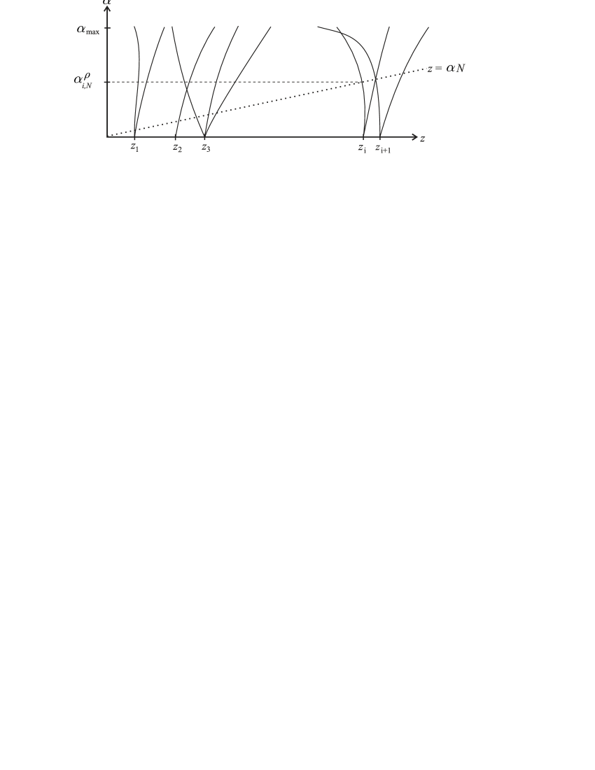
Figure 2. The solutions of $\det(I-U(z,\alpha))=0$

Proof.

Theorem 29 shows that $Z$ is everywhere locally a union of graphs of analytic functions, and these can be patched to functions on all of $[0,\alpha_{\rm{max}}]$. The theorem gives also the projections. Applying the theorem at $(z_{i},0)$ gives (59).

It remains to prove (61). If $z(\alpha)=z_{i}^{\rho}(\alpha)$ and $\varphi(\alpha)\in\operatorname{Ran}P_{i}^{\rho}(\alpha)$ is normalized and chosen analytic in $\alpha$ then differentiating $U(z(\alpha),\alpha)\varphi(\alpha)=\varphi(\alpha)$ gives $z^{\prime}(\partial_{z}U)\varphi+(\partial_{\alpha}U)\varphi+U\varphi^{\prime}=\varphi^{\prime}$. Taking the scalar product with $\varphi$ one obtains, since $\langle U\varphi^{\prime},\varphi\rangle=\langle\varphi^{\prime},U^{-1}\varphi\rangle=\langle\varphi^{\prime},\varphi\rangle$, that $z^{\prime}\langle(\partial_{z}U)\varphi,\varphi\rangle+\langle(\partial_{\alpha}U)\varphi,\varphi\rangle=0$ and hence, using $\varphi=U^{-1}\varphi$ and (57),

$$z^{\prime}=-\frac{\langle e^{iz2L}\frac{1}{i}\sigma S^{\prime}(\alpha)\varphi,\varphi\rangle}{\langle 2L\varphi,\varphi\rangle},$$

which is uniformly bounded as claimed. ∎

We now study the solutions of (54) and for this the intersection of $Z$ with the line $z=\alpha N$, for fixed $N$. The following is quite obvious from Figure 2.

Theorem 15.

• Fix arbitrary $i,\rho$. Then there is a unique point

  (63) $$(\alpha_{i,N}^{\rho},z_{i,N}^{\rho})=\text{ intersection point of }z=z_{i}^{\rho}(\alpha)\text{ and }z=\alpha N$$

  whenever $N\geq N_{0,i}:=C_{0}+\frac{z_{i}}{\alpha_{\rm{max}}}$ with $C_{0}$ from (61).

  Furthermore, $z_{i,N}^{\rho}$ is real analytic in $\frac{1}{N}$, i.e. $z_{i,N}^{\rho}=Z_{i}^{\rho}(\frac{1}{N})$ for a function $Z_{i}^{\rho}$ which is real analytic on $[0,(N_{0,i})^{-1}]$. Also, $Z_{i}^{\rho}(0)=z_{i}$.

• The pairs $(\alpha,\varphi)$, $0<\alpha\leq\alpha_{\rm{max}}$, for which $\Pi E_{\alpha,\varphi}$ satisfies the matching conditions (24) are given by

  (64) $$\alpha =\alpha_{i,N}^{\rho}=\frac{1}{N}z_{i,N}^{\rho}$$

  (65) $$\varphi \in{\mathcal{P}}_{\alpha,N}:=\bigoplus_{i,\rho:\,\alpha^{\rho}_{i,N}=\alpha}\operatorname{Ran}P_{i}^{\rho}(\alpha)$$

  for $i=1,2,\dots$ satisfying $N\geq N_{0,i}$ and $\rho=1,\dots,r_{i}$. The $P_{i}^{\rho}$ are defined in Proposition 14.

Proof.

(a) Fix $i,\rho$. The $z$-coordinates of the intersection points (63) are the solutions of $z=z_{i}^{\rho}(tz)$, where $t=\frac{1}{N}$, that is, the zeroes of the function $d(z)=z-z_{i}^{\rho}(tz)$. We have $d(0)=-z_{i}<0$ and $d(\frac{\alpha_{\rm{max}}}{t})=\frac{\alpha_{\rm{max}}}{t}-z_{i}^{\rho}(\alpha_{\rm{max}})\geq 0$ for $t\leq t_{\rm{max}}:=(N_{0,i})^{-1}$ since $z_{i}^{\rho}(\alpha_{\rm{max}})\leq z_{i}+C_{0}\alpha_{\rm{max}}$ by integration of the bound (61). Therefore, $d$ has a zero $z$ for each $t\leq t_{\rm{max}}$. The zero $z$ is unique since $d^{\prime}(z)=1-t(z_{i}^{\rho})^{\prime}(tz)>0$ for $t<1/C_{0}$ (which is satisfied for $t\leq t_{\rm{max}}$). Clearly, for $t=0$ the solution is $z=z_{i}$ by (59), and the inverse function theorem gives the analytic dependence on $t$.

(b) By Lemma 12, $\Pi E_{\alpha,\varphi}$ satisfies the matching conditions iff (54) is satisfied. The claim then follows from Proposition 14. ∎

A more precise analysis yields the uniform behavior of the functions $Z_{i}^{\rho}$ with respect to $i\to\infty$: $Z_{i}^{\rho}(t)=z_{i}+h_{i}^{\rho}(tz_{i})$ for functions $h_{i}^{\rho}$ which vanish at zero and have bounds on their derivatives independent of $i$. We will omit the proof since we don’t need it. Instead, we prove the following slightly weaker consequence of Theorem 15 about special regimes of solutions:

Theorem 16.

Given $\alpha_{0}\in[0,\alpha_{\rm{max}}]$ and $\delta>0$, $C>0$, the values of $\alpha$ in (64) in the interval $|\alpha-\alpha_{0}|<CN^{-\delta}$ satisfy

(66) $$\alpha=\frac{b_{i}^{\rho}}{N}+O(\frac{1}{N^{1+\delta}})$$

where $b_{i}^{\rho}=z_{i}^{\rho}(\alpha_{0})$, that is, $b=b_{i}^{\rho}$ are the solutions of

(67) $$\det(I-e^{ib2L}\sigma S(\alpha_{0}))=0,$$

and only the range $|b_{i}^{\rho}-N\alpha_{0}|<CN^{1-\delta}$ is considered. The constant implied in (66) is uniform in $i,\rho,N$ and $\delta$.

In particular, for $\alpha_{0}=0,$ $\delta=1$ we get: The solutions $\alpha$ with $\alpha<C/N$ are of the form

(68) $$\alpha=\frac{z_{i}}{N}+O(\frac{1}{N^{2}})$$

This is already clear from Theorem 15a).

Proof.

Let $t=1/N$. If $\alpha=\alpha_{i}^{\rho}(t)$ satisfies $|\alpha-\alpha_{0}|<Ct^{\delta}$ then $|z_{i}^{\rho}(\alpha)-z_{i}^{\rho}(\alpha_{0})|<C_{0}Ct^{\delta}$ by (61). From $\alpha=tz_{i}^{\rho}(\alpha)$ it then follows that $|\alpha-tb_{i}^{\rho}|<C_{0}Ct^{\delta+1}$, that is, (66). Finally, this estimate and $|\alpha-\alpha_{0}|<Ct^{\delta}$ imply $|tb_{i}^{\rho}-\alpha_{0}|<Ct^{\delta}(1+C_{0}t)$, and this yields the restricted range for $b_{i}^{\rho}$. ∎

We will also need the following stable version of Theorem 15b).

Theorem 17.

Let $N>0$. Assume $\alpha\in(0,\alpha_{\rm{max}})$ and $\varphi\in V$ are such that $\Pi E_{\alpha,\varphi}$ satisfies the matching conditions up to an error

(69) $$\|\operatorname{MC}_{\alpha}(E_{\alpha,\varphi})\|_{V}\leq\delta\|\varphi\|_{V},$$

for some $\delta>0$.

1. Then there is $i$, $\rho$ with

   (70) $$|\alpha-\alpha_{i,N}^{\rho}| \leq\frac{2}{l_{\operatorname{min}}}\frac{\delta}{N}.$$

2. Furthermore, there is $C>0$ such that, if $\delta<C^{-1}$ and $N>C$, then the sum ${\mathcal{P}}_{\alpha,\delta,N}=\bigoplus_{\beta}{\mathcal{P}}_{\beta,N}$, with $\beta$ ranging over $|\alpha-\beta|\leq N^{-1}\sqrt{\delta}$, is direct and, if $P$ is the projection to ${\mathcal{P}}_{\alpha,\delta,N}$, then

   (71) $$\|\varphi-P\varphi\|_{V}\leq\delta^{1/(2+2\dim V)}\,\|\varphi\|_{V}$$

Proof.

By (55) we have $e^{i\alpha NL}\operatorname{MC}_{\alpha}(E_{\alpha,\varphi})=\left(I-e^{i\alpha N2L}\sigma S(\alpha)\right)\varphi,$ so (69) implies $\|(I-e^{i\alpha N2L}\sigma S(\alpha))\varphi\|\leq\delta\|\varphi\|$. Write $z=\alpha N$ and

(72) $$U(z)=e^{iz2L}\sigma S(\frac{z}{N}),$$

then this reads

(73) $$\|(I-U(z))\varphi\|\leq\delta\,\|\varphi\|.$$

Now $z\mapsto U(z)$ is a monotone unitary family in the sense of (130), (131) since, with a prime denoting derivative in $z$,

$$\frac{1}{i}U^{\prime}U^{-1}=2L+\frac{1}{iN}US^{-1}S^{\prime}U^{-1}$$

where $U$ is evaluated at $z$ and $S$ at $z/N$, and for $N$ sufficiently large and $\alpha=z/N$ bounded this is positive with bounds as in (131), where ${d_{\text{min}}}$ can be taken as $l_{\operatorname{min}}$.

Therefore, we can apply Lemma 28 with $\varepsilon=\delta$. (70) follows from (135) (remember $\alpha=z/N$) and (71) from (136). ∎

6. Elliptic estimates

We first state some fairly standard elliptic estimates on the ’compact part’

$$X^{0}:=\bigcup_{v\in V}X_{v}$$

of $X^{\infty}$. Since we consider the scattering theory results in Section 4 as a black box in this article, we derive them from those results. In a more thorough and systematic treatment, they could be derived directly from the theory of elliptic boundary value problems and then used to derive the scattering theory results. However, the boundary value problem is slightly non-standard since it involves a non-local (pseudo-differential) boundary operator.

The boundary $\partial X^{0}$ splits in two parts: The part where the cylinders $Z^{N}$ are attached, which we may identify with $Y$ (which we sometimes also call $\{x=0\}$), and the complement $\partial X^{0}\setminus Y$. At the latter, we have boundary conditions given by the D/N decomposition (resp. Robin data). At $Y$ we will now impose boundary conditions motivated from the scattering theory.

For $u\in C^{\infty}(X^{0})$ and $\lambda<\nu_{1}$ let

$$B_{\perp}(\lambda)u:=\Pi^{\perp}\partial_{\xi}u_{|Y}-Q(\lambda)(\Pi^{\perp}u_{|Y}),$$

where for $\varphi_{k}\in V_{k}$, $k\in\mathbb{N}$,

$$Q(\lambda)(\sum_{k=1}^{\infty}\varphi_{k}):=-\sum_{k=1}^{\infty}\sqrt{\nu_{k}-\lambda}\varphi_{k},$$

if the sums converge. $Q(\lambda)$ is the $\Pi^{\perp}$ part of the Dirichlet to Neumann operator for exponentially decreasing solutions of $(\Delta_{Z^{\infty}}+\lambda)\tilde{u}=0$, see (29). Thus, $B_{\perp}(\lambda)u=0$ iff $\Pi^{\perp}\tilde{u}$ has no exponentially increasing part, where $\tilde{u}$ is the unique function on $Z^{\infty}$ satisfying $(\Delta_{Z^{\infty}}+\lambda)\tilde{u}=0$ and having the same value and normal derivative at $x=0$ as $u$ at $Y$.

Consider the operator $\Delta_{X^{0}}$ with domain $\operatorname{Dom}(\Delta_{X^{0}})\subset H^{2}(X^{0})$ defined by the D/N boundary conditions (resp. Robin data) at $\partial X^{0}\setminus Y$. In order to obtain a selfadjoint extension of $\Delta_{X^{0}}$ we need in addition to impose boundary conditions at $Y$. In addition to the condition $B_{\perp}(\lambda)u=0$ we need a condition involving $u^{0}:=\Pi u_{|Y}$, $u^{1}:=\Pi\partial_{\xi}u_{|Y}$. It is well-known and easy to check that selfadjoint boundary conditions correspond to subspaces ${\mathcal{L}}\subset V\times V$ which are Lagrangian, i.e. such that $\dim{\mathcal{L}}=\dim V$ and

$$(u^{0},u^{1}),(v^{0},v^{1})\in{\mathcal{L}}\Longrightarrow\langle u^{0},v^{1}\rangle-\langle v^{0},u^{1}\rangle=0.$$

Thus, for ${\mathcal{L}}$ Lagrangian and any $\lambda$ the operator $\Delta_{X^{0}}$ is selfadjoint on the domain $\{u\in\operatorname{Dom}(\Delta_{X^{0}}:\,B_{\perp}(\lambda)=0,\,(u^{0},u^{1})\in{\mathcal{L}}\}$.

We have the following elliptic estimates.

Lemma 18.

Let $\alpha\in[0,\alpha_{\rm{max}}]$. Assume $\lambda=\nu+\alpha^{2}$ is not an $L^{2}$ eigenvalue of $-\Delta_{X^{\infty}}$. Let ${\mathcal{L}}_{\alpha}$ be the scattering subspace (46), and let ${\mathcal{L}}_{\alpha}^{\prime}$ be a Lagrangian subspace of $V\times V$ such that ${\mathcal{L}}_{\alpha}\cap{\mathcal{L}}^{\prime}_{\alpha}=\{0\}$. Also, let $P_{{\mathcal{L}}_{\alpha},{\mathcal{L}}^{\prime}_{\alpha}}:V\times V\to{\mathcal{L}}_{\alpha}$ be the projection along ${\mathcal{L}}_{\alpha}^{\prime}$. There is a constant $C$ so that if $u\in C^{\infty}(X^{0})$ satisfies the D/N (resp. Robin) boundary conditions at $\partial X^{0}\setminus Y$ and

(74) $$(\Delta+\lambda)u =f \text{ in }X^{0}$$

$$B_{\perp}(\lambda)u =g \text{ at }Y$$

$$P_{{\mathcal{L}}_{\alpha},{\mathcal{L}}^{\prime}_{\alpha}}(u^{0},u^{1}) =h$$

then

(75) $$\|u\|_{H^{2}(X^{0})}\leq C(\;\|f\|_{L^{2}(X^{0})}+\|g\|_{H^{1/2}(Y)}+\|h\|_{V\times V}\;).$$

If $\alpha$ is varied and the ${\mathcal{L}}_{\alpha}^{\prime}$ depend continuously on $\alpha$ then the constant $C$ can be chosen independent of $\alpha$.

See Section 7.4 for a replacement in case $\nu+\alpha^{2}$ is an $L^{2}$-eigenvalue.

Proof.

If $u$ is a solution of the homogeneous problem, i.e. $f=0$, $g=0$, $h=0$, then $g=0$ implies that $u$ extends to a solution of $(\Delta+\lambda)u=0$ on $X^{\infty}$ with bounded $\Pi^{\perp}$ part and hence that $u$ is a scattering solution. Then $(u^{0},u^{1})\in{\mathcal{L}}_{\alpha}$ by definition of ${\mathcal{L}}_{\alpha}$. $h=0$ implies $(u^{0},u^{1})\in{\mathcal{L}}^{\prime}_{\alpha}$, hence $(u^{0},u^{1})=0$ since ${\mathcal{L}}_{\alpha}\cap{\mathcal{L}}^{\prime}_{\alpha}=\{0\}$ and therefore $u\equiv 0$ by uniqueness of scattering solutions.

Therefore, the map $u\mapsto((\Delta+\lambda)u,B_{\perp}(\lambda)u,P_{{\mathcal{L}}_{\alpha},{\mathcal{L}}^{\prime}_{\alpha}}(u^{0},u^{1})),\ \operatorname{Dom}(\Delta_{X^{0}})\to L^{2}(X^{0})\times H^{1/2}(Y)\times(V\times V)$ is injective. It is also surjective, since for $g=0$, $h=0$ one has a solution $u$ for any $f$ by the Fredholm alternative (since the operator $\Delta_{X^{0}}+\lambda$ is selfadjoint on the domain which consists of those $u$ satisfying homogeneous boundary conditions, has closed range and is injective), and arbitrary $g,h$ can be removed by replacing $u$ by $u-v$, where $v$ is any function in $\operatorname{Dom}(\Delta_{X^{0}})$ satisfying $B_{\perp}(\lambda)v=g$, $P_{{\mathcal{L}}_{\alpha},{\mathcal{L}}^{\prime}_{\alpha}}(v^{0},v^{1})=h$. $v$ exists by standard arguments, since $X^{0}$ is of product type near $Y$ by assumption. Since $\operatorname{Dom}(\Delta_{X^{0}})$ is complete with the $H^{2}$-norm the open mapping theorem gives (75).

To show that $C$ can be chosen independent of $\alpha$ it suffices to show that it can be chosen locally uniformly with respect to $\alpha$. This can be proved as follows: Fix $\alpha_{0}$ and let $C_{0}$ be the constant for $\alpha=\alpha_{0}$. Suppose $u$ satisfies (74) for some $\alpha$ near $\alpha_{0}$. This can be rewritten $(\Delta+\lambda_{0})u=f+(\lambda_{0}-\lambda)u,\ B_{\perp}(\lambda_{0})u=g+(B_{\perp}(\lambda_{0})-B_{\perp}(\lambda))u,P_{{\mathcal{L}}_{\alpha_{0}},{\mathcal{L}}^{\prime}_{\alpha_{0}}}(u^{0},u^{1})=h+(P_{{\mathcal{L}}_{\alpha_{0}},{\mathcal{L}}^{\prime}_{\alpha_{0}}}-P_{{\mathcal{L}}_{\alpha},{\mathcal{L}}^{\prime}_{\alpha}})(u^{0},u^{1})$. Estimate (75) with these data yields $\|u\|_{H^{2}(X^{0})}\leq C_{0}(\;\|f\|_{L^{2}(X^{0})}+\|g\|_{H^{1/2}(Y)}+\varepsilon\|u\|_{H^{2}(X^{0})})$, where $\varepsilon\to 0$ as $\alpha\to\alpha_{0}$ (independently of $u$), since all operators on the right in (74) depend continuously on $\alpha$. For $\varepsilon<1/2C_{0}$ the last term can be absorbed into the left hand side, and the claim follows. ∎

Using (75) with $u=E$ a scattering solution we get

(76) $$\|E\|_{H^{2}(X^{0})}\leq C\|(E^{0},E^{1})\|_{V\times V}\quad\text{ for any scattering solution }E.$$

When applying Lemma 18 we will need the following estimate which shows that the exponentially increasing part, $B_{\perp}(\lambda)u$, of an eigenfunction on $X^{N}_{G}$ is very small.

Lemma 19.

Let $(\Delta_{X_{G}^{N}}+\mu)u=0$, $\mu<\nu_{1}$. Then

(77) $$\|B_{\perp}(\mu)u\|_{H^{1/2}(Y)}\leq Ce^{-cN}\|u\|_{H^{2}(X^{0})}.$$

Proof.

If $\Pi^{\perp}u=\sum_{k=1}^{\infty}e^{-\sqrt{\nu_{k}-\mu}\xi}\varphi_{k}+e^{\sqrt{\nu_{k}-\mu}\xi}\psi_{k}$ with $\varphi_{k},\psi_{k}\in V_{k}$ then $B_{\perp}(\mu)u=\sum_{k=1}^{\infty}\sqrt{\nu_{k}-\mu}\psi_{k}$. Since $\Delta_{Y}$ is an elliptic operator of order $2$, with eigenvalues $\nu_{k}$, it follows that $\|B_{\perp}(\mu)u\|_{H^{1/2}(Y)}\leq\|\sum_{k=1}^{\infty}({\nu_{k}})^{1/4}\sqrt{\nu_{k}-\mu}\psi_{k}\|_{L^{2}(Y)}$, and then (32) together with the trace theorem gives the claim. ∎

We will need that scattering solutions for different spectral values whose leading parts satisfy the matching conditions are almost orthogonal on $X^{N}$:

Lemma 20.

Let $\alpha,\alpha^{\prime}\in A_{N}$ and $\varphi\in{\mathcal{P}}_{\alpha,N},\varphi^{\prime}\in{\mathcal{P}}_{\alpha^{\prime},N}$. If $\alpha\neq\alpha^{\prime}$ then the restrictions of $E=E_{\alpha,\varphi},E^{\prime}=E_{\alpha^{\prime},\varphi^{\prime}}$ to $X^{N}$ are almost orthogonal, i.e.

$$|\langle E,E^{\prime}\rangle_{X^{N}}|\leq Ce^{-cN}\|E\|_{X^{N}}\|E^{\prime}\|_{X^{N}}.$$

Proof.

With $\lambda=\nu+\alpha^{2},\ \lambda^{\prime}=\nu+(\alpha^{\prime})^{2}$ we have by Green’s formula

$$(\lambda-\lambda^{\prime})\langle E,E^{\prime}\rangle_{X^{N}} =\langle\lambda E,E^{\prime}\rangle_{X^{N}}-\langle E,\lambda^{\prime}E^{\prime}\rangle_{X^{N}}=-\langle\Delta E,E^{\prime}\rangle_{X^{N}}+\langle E,\Delta E^{\prime}\rangle_{X^{N}}$$

$$=\langle E_{x=N},\partial_{\xi}E^{\prime}_{x=N}\rangle_{Y}-\langle\partial_{\xi}E_{x=N},E^{\prime}_{x=N}\rangle_{Y}$$

Since $\Pi E$, $\Pi E^{\prime}$ satisfy the matching conditions at $x=N$, the $\Pi$ part of the latter scalar products vanishes, and only the $\Pi^{\perp}$ part remains. Writing $\Pi^{\perp}E=\sum_{k=1}^{\infty}e^{-\sqrt{\nu_{k}-\lambda}Lx}\varphi_{k}$, $\varphi_{k}\in V_{k}$, and similarly for $\Pi^{\perp}E^{\prime}$, we get

$$(\lambda-\lambda^{\prime})\langle E,E^{\prime}\rangle_{X^{N}} =\sum_{k=1}^{\infty}(\sqrt{\nu_{k}-\lambda}-\sqrt{\nu_{k}-\lambda^{\prime}})\langle e^{-\sqrt{\nu_{k}-\lambda}LN}\varphi_{k},e^{-\sqrt{\nu_{k}-\lambda^{\prime}}LN}\varphi_{k}^{\prime}\rangle$$

$$=(\lambda^{\prime}-\lambda)\sum_{k=1}^{\infty}(\sqrt{\nu_{k}-\lambda}+\sqrt{\nu_{k}-\lambda^{\prime}})^{-1}\langle e^{-\sqrt{\nu_{k}-\lambda}LN}\varphi_{k},e^{-\sqrt{\nu_{k}-\lambda^{\prime}}LN}\varphi_{k}^{\prime}\rangle,$$

and since the latter sum is bounded by

$$Ce^{-cN}\sqrt{\sum_{k}\|\varphi_{k}\|^{2}}\sqrt{\sum_{k}\|\varphi_{k}^{\prime}\|^{2}}=Ce^{-cN}\|\Pi^{\perp}E_{x=0}\|_{Y}\|\Pi^{\perp}E^{\prime}_{x=0}\|_{Y}$$

and since $\|E_{x=0}\|\leq C\|E\|_{X^{0}}$ by elliptic regularity, the claim follows. ∎

7. Proof of the Main Theorem

In this section we prove the main theorems. We treat separately the following cases: Eigenvalues on $X^{N}_{G}$ arising from $L^{2}-$eigenvalues on $X^{\infty}$ below the essential spectrum; eigenvalues on $X^{N}_{G}$ arising from the continuous spectrum on $X^{\infty}$ but away from the threshold, i.e. bigger than $\nu+e^{-cN}$ for suitable $c>0$; eigenvalues on $X^{N}_{G}$ arising from the threshold.

In each case, the proof proceeds in two steps: In Step 1, we construct the eigenvalues on $X^{N}_{G}$ from approximate eigenfunctions constructed from the (generalized) eigenfunctions on $X^{\infty}$. In Step 2 we show that in this way all eigenfunctions are obtained.

We assume at first there $-\Delta_{X^{\infty}}$ has no $L^{2}$-eigenvalues in $[\nu,\lambda_{\rm max}]$. The modifications needed in case there are such eigenvalues are described in Section 7.4.

We use the following notation: For a selfadjoint operator $A$ and $I\subset\mathbb{R}$ let ${\rm Eig}_{I}(A)$ be the spectral subspace for the spectral interval $I$. If $A$ has only discrete spectrum in $I$, this is the span of the eigenfunctions of $A$ with eigenvalues in $I$. Also, let

$${\rm Eig}_{I,N}:={\rm Eig}_{I}(-\Delta_{X_{G}^{N}}).$$

We will construct approximate spectral subspaces ${\rm Eig}^{{\rm app}}_{I,N}$, defined in each case separately, using a cutoff function defined as follows. Choose $\chi\in C^{\infty}(\mathbb{R})$ satisfying $\chi(x)=1$ for $x\leq-\frac{1}{2}$ and $\chi(x)=0$ for $x\geq-\frac{1}{3}$ and set

(78) $$\chi_{N}(x)=\chi(x-N).$$

Thus, if $u$ is a function on $X^{N}$ then $\chi_{N}u$ equals $u$ for $x\leq N-1$ and is identically zero for $x\geq N-\frac{1}{3}$.

Note that one could not hope to approximate individual eigenfunctions on $X^{N}_{G}$ by approximate eigenfunctions if the eigenvalues lie very close together.

7.1. Eigenvalues arising from $L^{2}$ eigenvalues on $X^{\infty}$

For $I\subset(0,\nu)$ let

(79) $${\rm Eig}^{{\rm app}}_{I,N}:=\operatorname{span}\{\chi_{N}u:\,u\in{\rm Eig}_{I}(-\Delta_{X^{\infty}})\}.$$

Theorem 21.

For any $c_{0}>0$ there is $N_{0}>0$ such that for $N\geq N_{0}$ the eigenvalues $\mu\leq\nu-c_{0}$ of $-\Delta_{X_{G}^{N}}$ lie within $Ce^{-cN}$ of the $L^{2}$-eigenvalues of $-\Delta_{X^{\infty}}$.

For each $L^{2}$-eigenvalue $\lambda<\nu$ of $-\Delta_{X^{\infty}}$ we have

(80) $$\operatorname{dist}_{\rm{symm}}({\rm Eig}_{I,N},{\rm Eig}^{{\rm app}}_{\{\lambda\},N})\leq Ce^{-cN},\quad I=(\lambda-Ce^{cN},\lambda+Ce^{-cN}).$$

Here $c=\sqrt{\nu-\lambda_{\rm max}}$ where $\lambda_{\rm max}$ is the largest eigenvalue of $-\Delta_{X^{\infty}}$ less than $\nu$.

Proof.

Step 1: Show that the approximate eigenfunctions are actually such:

(81) $$\operatorname{dist}({\rm Eig}^{{\rm app}}_{\{\lambda\},N},{\rm Eig}_{I,N})<1.$$

In particular, $-\Delta_{X_{G}^{N}}$ has at least $\dim{\rm Eig}^{{\rm app}}_{\{\lambda\},N}$ many eigenvalues in $I$.

Proof: Let $W={\rm Eig}^{{\rm app}}_{\{\lambda\},N}$. For $w=\chi_{N}u\in W$ one has

$$\Delta w=\chi_{N}(\Delta u)+2\nabla\chi_{N}\nabla u+(\Delta\chi_{N})u=-\lambda\chi_{N}u+2L^{-2}\chi_{N}^{\prime}\partial_{x}u+L^{-2}\chi_{N}^{\prime\prime}u,$$

and since $\chi_{N}^{\prime},\chi_{N}^{\prime\prime}$ are supported in $(N-1,N)$, one obtains from (30), applied with $M\in(N-1,N)$, that

(82) $$\|(\Delta_{X^{N}_{G}}+\lambda)w\|_{X^{N}_{G}}\leq Ce^{-cN}\|w\|_{X^{N}_{G}}.$$

Since $W\subset\operatorname{Dom}(\Delta_{X^{N}_{G}})$ we may apply the Spectral Approximation Lemma 7 to the operator $A=-\Delta_{X^{N}_{G}}$, with $\lambda_{0}=\lambda$ and $\varepsilon=Ce^{-cN},\delta=2\varepsilon$, and this gives (81).

Step 2: Show that any eigenvalue $\mu$ of $-\Delta_{X_{G}^{N}}$ is in some $I=(\lambda-Ce^{cN},\lambda+Ce^{-cN})$ and that

(83) $$\operatorname{dist}({\rm Eig}_{I,N},{\rm Eig}^{{\rm app}}_{\{\lambda\},N})\leq Ce^{-cN}.$$

Proof: Let $u$ be an eigenfunction of $-\Delta_{X^{N}_{G}}$, with eigenvalue $\mu\leq\nu-\gamma$. Then $w=\chi_{N}u\in\operatorname{Dom}(\Delta_{X^{\infty}})$ satisfies (with $c_{1}=\sqrt{\gamma}$)

$$\|(\Delta_{X^{\infty}}+\mu)w\|_{X^{\infty}}\leq Ce^{-c_{1}N}\|w\|_{X^{\infty}}.$$

This follows from exponential decay of $w$ and is proved in the same way as (82). This implies $|\mu-\lambda|\leq Ce^{-c_{1}N}$ for some $\lambda\in\operatorname{spec}(-\Delta_{X^{\infty}})$ (in particular, $c_{1}$ may be replaced by $c$). Since $\mu\leq\nu-\gamma$, $\lambda$ must be an $L^{2}$ eigenvalue of $-\Delta_{X^{\infty}}$. Now apply the Spectral Approximation Lemma 7 to $A=-\Delta_{X^{\infty}}$, $W=\operatorname{span}\{w\}$, with $\lambda_{0}=\mu$ and $\varepsilon=Ce^{-cN}$, $\delta=\operatorname{dist}(\mu,\operatorname{spec}(-\Delta_{X^{\infty}})\setminus\{\lambda\})$. Since the interval $(\mu-\delta,\mu+\delta)$ intersects the spectrum of $-\Delta_{X^{\infty}}$ only in $\lambda$, we get $\operatorname{dist}(\operatorname{span}\{w\},{\rm Eig}_{\{\lambda\}}(-\Delta_{X^{\infty}}))<Ce^{-cN}$, and this implies (using exponential decay again)

(84) $$\operatorname{dist}(\operatorname{span}\{u\},{\rm Eig}^{{\rm app}}_{\{\lambda\},N})\leq Ce^{-cN}.$$

Finally, applying this to an orthonormal basis of eigenfunctions of $-\Delta_{X_{G}^{N}}$ with eigenvalues in $I$, we get (83) from (37).

End of proof: The first statement of the theorem is contained in Step 2, and (81) and (83) together imply (80) by Lemma 6c). ∎

7.2. Eigenvalues arising from the interior of the continuous spectrum

To define the approximate eigenspaces, recall Theorem 15. Let

$$A_{N}=\{\alpha_{i,N}^{\rho}:\,i=1,2,\dots;\rho=1,\dots,r_{i},\ \alpha_{i,N}^{\rho}\in(0,\alpha_{\rm{max}}]\},\quad\Lambda_{N}=\{\nu+\alpha^{2}:\,\alpha\in A_{N}\}.$$

Recall that $\alpha\in A_{N}$ iff $\Pi E_{\alpha,\varphi}$ satisfies the matching conditions for some $\varphi\neq 0.$ The corresponding space of $\varphi$ is ${\mathcal{P}}_{\alpha,N}$ from (65). Therefore, the function

(85) $$\tilde{E}_{\alpha,\varphi}=\begin{cases}E_{\alpha,\varphi}&\text{ on }X^{0}\\ \Pi E_{\alpha,\varphi}+\chi_{N}\Pi^{\perp}E_{\alpha,\varphi}&\text{ on }Z^{N}\end{cases}$$

is smooth on $X^{N}_{G}$ and in the domain of $\Delta_{X_{G}^{N}}$.

For $I\subset\mathbb{R}$ let

$${\rm Eig}^{{\rm app}}_{I,N}:=\operatorname{span}\{\tilde{E}_{\alpha,\varphi},\ \nu+\alpha^{2}\in I,\ \alpha\in A_{N},\ \varphi\in{\mathcal{P}}_{\alpha,N}\}.$$

Also, if $I=(A,B)$ and $\delta>0$ then let

$$I_{\delta}:=(A-\delta,B+\delta).$$

We call $\dim{\mathcal{P}}_{\alpha,N}$ the multiplicity of $\alpha$ resp. of $\lambda=\nu+\alpha^{2}$.

Theorem 22.

Assume $-\Delta_{X^{\infty}}$ has no $L^{2}$-eigenvalues in $[\nu,\lambda_{\rm max}]$. The numbers $\lambda\in\Lambda_{N}$ are the approximate eigenvalues of $-\Delta_{X_{G}^{N}}$, with approximate eigenfunctions linear combinations of $\tilde{E}_{\alpha,\varphi}$, $\varphi\in{\mathcal{P}}_{\alpha,N}$. The errors are of order $e^{-cN}$.

More precisely, given a sufficiently small $c_{0}>0$ there are constants $C,c>0$ such that:

1. Let $\mu_{i}$ be the eigenvalues bigger than $\nu+e^{-2c_{0}N}$ of $-\Delta_{X_{G}^{N}}$, arranged in increasing order and counted with multiplicity. Also, let $\lambda_{i}$ be the elements of $\Lambda_{N}$, arranged in increasing order and counted with multiplicity. Then, for all $i$,

   (86) $$|\lambda_{i}-\mu_{i}|\leq Ce^{-cN}.$$

2. Let $I\subset(\nu+Ce^{-cN},\lambda_{\rm max}]$. If there is no $\lambda\in\Lambda_{N}$ in $I_{2Ce^{-cN}}\setminus I$ then

   (87) $$\operatorname{dist}_{\rm{symm}}({\rm Eig}_{I^{\prime},N},{\rm Eig}^{{\rm app}}_{I,N})\leq Ce^{-cN},\quad I^{\prime}=I_{Ce^{-cN}}.$$

See Section 7.4 for the modifications needed in case there are $L^{2}$-eigenvalues in $[\nu,\lambda_{\rm max}]$.

The statement in b) is complicated due to the possible crossings of the branches $z_{i}^{\rho}$ for different $i$ in Figure 2. These do not occur on the line $z=\alpha N$ for bounded $i$ (corresponding to fixed $k$ as in Theorem 1), and one obtains:

Corollary 23.

The eigenvalues of $-\Delta_{X_{G}^{N}}$ form clusters of width $Ce^{-cN}$ around the $\lambda\in\Lambda_{N}$. For any $C_{0}>0$ there are $c>0,N_{0}$ such that for $N\geq N_{0}$ the clusters around the $\lambda\leq\nu+C_{0}N^{-2}$ are disjoint and the span of eigenfunctions of $-\Delta_{X_{G}^{N}}$ corresponding to the $\lambda$-cluster has distance less than $e^{-cN}$ from

$$\operatorname{span}\{\tilde{E}_{\alpha,\varphi}:\varphi\in{\mathcal{P}}(\alpha)\}$$

where $\lambda=\nu+\alpha^{2}$, ${\mathcal{P}}(\alpha)=\ker(I-e^{i\alpha N2L}\sigma S(\alpha))$.

Proof.

The first statement is just (86). There are only a bounded number of $\lambda\in\Lambda_{N}$ satisfying $\lambda\leq\nu+C_{0}N^{-2}$ by the Weyl asymptotics (58). They are polynomially separated, i.e. there are $K\in\mathbb{N},c>0$ (depending on $C_{0}$) so that $|\lambda-\lambda^{\prime}|\geq cN^{-K}$ for any two different such values, by Theorem 15 and the fact that the $Z_{i}^{\rho}$ are different analytic functions. This implies the disjointness of clusters for large $N$ and that the separation condition in Theorem 22b) is satisfied for $I=\{\lambda\}$, and this gives the last claim. ∎

Proof of Theorem 22.

As always, we write $\lambda=\nu+\alpha^{2}$.

Step 1: Show that the approximate eigenfunctions are actually such: For any intervals as in the theorem we have, for $C$ sufficiently large,

(88) $$\operatorname{dist}({\rm Eig}^{{\rm app}}_{I,N},{\rm Eig}_{I^{\prime},N})<1.$$

Proof: Let $\lambda\in\Lambda_{N}$ and let $W_{\lambda}={\rm Eig}^{{\rm app}}_{\{\lambda\},N}$. For $w=\tilde{E}_{\alpha,\varphi}\in W_{\lambda}$ one has

$$\Delta w=-\lambda w+2L^{-2}\chi_{N}^{\prime}\partial_{x}\Pi^{\perp}E_{\alpha,\varphi}+L^{-2}\chi_{N}^{\prime\prime}\Pi^{\perp}E_{\alpha,\varphi},$$

and since $\chi_{N}^{\prime},\chi_{N}^{\prime\prime}$ are supported in $(N-1,N)$, one obtains from (31), applied to $u=E_{\alpha,\varphi}$ with $M\in(N-1,N)$, that

(89) $$\|(\Delta_{X^{N}_{G}}+\lambda)w\|_{X^{N}_{G}}\leq Ce^{-cN}\|w\|_{X^{N}_{G}}.$$

Since $W_{\lambda}\subset\operatorname{Dom}(\Delta_{X^{N}_{G}})$ we may apply the Spectral Approximation Lemma 7 to the operator $A=-\Delta_{X^{N}_{G}}$, with $\lambda_{0}=\lambda$ and $\varepsilon=Ce^{-cN}$ and $\delta>0$ to be chosen, and this gives

(90) $$\operatorname{dist}({\rm Eig}^{{\rm app}}_{\{\lambda\},N},{\rm Eig}_{(\lambda-\delta,\lambda+\delta),N})\leq Ce^{-cN}/\delta.$$

If $\delta=2Ce^{-cN}$ then this is (88) with $I=\{\lambda\}$.

To obtain (88) for arbitrary $I$, first observe that (90) implies $\operatorname{dist}({\rm Eig}^{{\rm app}}_{\{\lambda\},N},{\rm Eig}_{J,N})\leq Ce^{-cN}/\delta$ for any interval $J$ containing $(\lambda-\delta,\lambda+\delta)$. Next, use Lemma 20 together with a version of (37) for almost orthogonal subspaces to conclude that $\operatorname{dist}({\rm Eig}^{{\rm app}}_{I,N},{\rm Eig}_{I_{\delta},N})\leq\sum\limits_{\lambda\in I\cap\Lambda_{N}}(\operatorname{dist}({\rm Eig}^{{\rm app}}_{\{\lambda\},N},I_{\delta})+Ce^{-cN})$. Since $\Lambda_{N}$ has at most $O(N)$ elements, the left hand side is bounded by $NCe^{-cN}/\delta$. Hence, choosing $\delta=2NCe^{-cN}$ (or $e^{-c^{\prime}N}$ with $c^{\prime}$ smaller than $c$ and $N$ large) one obtains (88).

Step 2: Show that each eigenvalue $\mu>\nu+e^{-2c_{0}N}$ of $-\Delta_{X_{G}^{N}}$ is exponentially close to some $\lambda\in\Lambda_{N}$ and that, under the assumptions of the theorem,

(91) $$\operatorname{dist}({\rm Eig}_{I^{\prime},N},{\rm Eig}^{{\rm app}}_{I,N})\leq Ce^{-cN}.$$

Proof: Let $(\Delta_{X_{G}^{N}}+\mu)u=0$, $\mu=\nu+\beta^{2}$, so $\beta>e^{-c_{0}N}$. For $E=E_{\alpha,\varphi}$ recall the notation $(E^{0},E^{1})=(\Pi E_{x=0},\Pi\partial_{\xi}E_{x=0})\in V\times V$. For $\alpha\in A_{N}$ denote

(92) $${\mathcal{F}}_{\alpha,N}=\{(E^{0},E^{1}):\,E=E_{\alpha,\varphi},\ \varphi\in{\mathcal{P}}_{\alpha,N}\}.$$

Step 2a: $(u^{0},u^{1})$ is close to ${\mathcal{L}}_{\beta}$ by the elliptic estimate:

(93) $$\operatorname{dist}(\operatorname{span}\{(u^{0},u^{1})\},{\mathcal{L}}_{\beta})\leq Ce^{-cN}.$$

Proof: Apply the basic elliptic estimate, Lemma 18, as follows: Let $(E^{0},E^{1})$ be the orthogonal projection of $(u^{0},u^{1})$ to ${\mathcal{L}}_{\beta}$. This corresponds to a scattering solution $E$ for spectral value $\mu$. Let $v=u-E$. From $(\Delta+\mu)E=0$, $B_{\perp}(\mu)E=0$ it follows that $v$ satisfies (74) with $f=0$, $g=B_{\perp}(\mu)u$, ${\mathcal{L}}_{\beta}^{\prime}=$ the orthogonal complement of ${\mathcal{L}}_{\beta}$ and $h=0$. From Lemma 19 it follows that $\|g\|_{H^{1/2}(Y)}\leq Ce^{-cN}\|u\|_{H^{2}(X^{0})}$, and then (75) gives

(94) $$\|v\|_{H^{2}(X^{0})}\leq Ce^{-cN}\|u\|_{H^{2}(X^{0})},\quad v=u-E.$$

This implies $\|u\|_{H^{2}(X^{0})}\leq C\|E\|_{H^{2}(X^{0})}$, and with (76) we get

(95) $$\|u\|_{H^{2}(X^{0})}\leq C\|(E^{0},E^{1})\|_{V\times V}.$$

Next, the trace theorem implies $\|(v^{0},v^{1})\|_{V\times V}\leq C\|v\|_{H^{2}(X^{0})}$, and so (94) gives

(96) $$\|(v^{0},v^{1})\|_{V\times V}\leq Ce^{-cN}\|(E^{0},E^{1})\|_{V\times V},$$

which after writing $E=u-v$ and absorbing the $v$ term into the left hand side gives $\|(v^{0},v^{1})\|_{V\times V}\leq Ce^{-cN}\|(u^{0},u^{1})\|_{V\times V},$ that is (93).

Step 2b: Use the matching conditions to show: (93) implies

(97) $$\operatorname{dist}(\beta,A_{N}) \leq Ce^{-cN}$$

(98) $$\operatorname{dist}(\operatorname{span}\{(u^{0},u^{1})\},\bigoplus_{\alpha\in A_{N}:|\alpha-\beta|<Ce^{-cN}}{\mathcal{F}}_{\alpha,N}) \leq Ce^{-cN}.$$

The ${\mathcal{F}}_{\alpha,N}$ are defined in (92).

Proof: Since $(\Delta_{X^{N}}+\mu)v=0$ one obtains from (36), using $|\cos{\beta N}|\leq 1,\ |\beta^{-1}\sin(\beta N)|\leq N$, that

$$\|\operatorname{MC}_{\beta}(v)\|_{V}\leq\|(v^{0}\|_{V}+(N+\frac{1}{\alpha})\|v^{1})\|_{V}\leq e^{c_{0}N}\|(v^{0},v^{1}\|_{V\times V}.$$

From $\operatorname{MC}_{\beta}(u)=0$ we have $\operatorname{MC}_{\beta}(E)=-\operatorname{MC}_{\beta}(v)$, and then (96) gives

(99) $$\|\operatorname{MC}_{\beta}(E)\|_{V}=\|\operatorname{MC}_{\beta}(v)\|_{V}\leq Ce^{-c_{1}N}\|(E^{0},E^{1})\|_{V\times V}.$$

where $c_{1}=c-c_{0}$. If $E=E_{\beta,\varphi}$ then clearly $\|(E^{0},E^{1})\|_{V\times V}\leq C\|\varphi\|_{V}$, so we can apply the Stability Theorem 17 with $\delta=Ce^{-c_{1}N}$ and obtain (97) with $c=c_{1}$, as well as $\operatorname{dist}(\operatorname{span}\{\varphi\},\bigoplus_{\alpha^{\prime}}{\mathcal{P}}_{\alpha^{\prime},N})\leq Ce^{-c_{2}N}$ where $c_{2}=c_{1}/(2+2\dim V)$ and the sum is over $\alpha^{\prime}\in A_{N}$ satisfying $|\alpha-\alpha^{\prime}|\leq Ce^{-c_{1}N/2}$. This implies that $(E^{0},E^{1})$ and hence, by (96), $(u^{0},u^{1})$ has distance at most $Ce^{-c_{2}N}$ from $\bigoplus_{\alpha^{\prime}}{\mathcal{F}}_{\alpha^{\prime},N}$, and hence (98), with $c=c_{2}$.

End of proof of Step 2: The estimate $\|v\|_{X^{N}}\leq CN\|(v^{0},v^{1})\|_{V\times V}$ for eigensolutions on $X^{N}$ which are a difference of a scattering solution and an eigenfunction on $X^{N}_{G}$ (use (31) and a modification of the derivation of (76)) shows that (98) implies

(100) $$\operatorname{dist}(\{u\},{\rm Eig}^{{\rm app}}_{J,N})\leq Ce^{-cN},\quad J=(\mu-Ce^{-cN},\mu+Ce^{-cN}).$$

Finally, we apply this to an orthonormal set of eigenfunctions $u$ with eigenvalues in $I^{\prime}$. Lemma 6e) gives $\operatorname{dist}({\rm Eig}_{I^{\prime},N},{\rm Eig}^{{\rm app}}_{I^{\prime\prime},N})\leq Ce^{-cN}$ with $I^{\prime\prime}=(I^{\prime})_{Ce^{-cN}}=I_{2Ce^{-cN}}$ and hence (91), since by assumption any $\lambda\in I^{\prime\prime}\cap\Lambda_{N}$ must already lie in $I$.

End of proof of Theorem 22: (88) and (91) give part b) of the Theorem by Lemma 6b). Part a) then follows easily: Since $\Lambda_{N}$ has $O(N)$ elements, we may cover it by intervals $I_{k}$ of length at most $CNe^{-cN}$, satisfying the hypothesis of b) (note that any $\lambda\in\Lambda_{N}$ is at least $\nu+cN^{-2}$ by (59),(64) since $z_{1}>0$). The $\mu_{i}$ must then be in the $Ce^{-cN}$-neighborhoods of the $I_{k}$ by b), and this implies a), with slightly smaller $c$. ∎

7.3. Eigenvalues close to the threshold $\nu$

Recall from Lemma 11 that $\Pi E_{0,\Phi_{+},\Psi_{-}}$ satisfies the matching conditions at $x=N$ iff $\sigma\Phi_{+}=\Phi_{+}$ and $\Psi_{-}=0$. Denote

$$V_{+}^{+}:=V_{+}\cap V^{+},\quad\Phi_{+}^{+}=\text{ the projection to }V_{+}^{+}\text{ of }\Phi\in V.$$

Note that, since $\sigma$ and $S(0)$ do not commute in general, some care is needed with this notation. For example, usually $\Phi_{+}\neq\Phi_{+}^{+}+\Phi_{+}^{-}$ (with $\Phi_{+}^{-}$ defined analogously).

For $\Phi\in V_{+}^{+}$ let

(101) $$\tilde{E}_{0,\Phi,0}:=\begin{cases}E_{0,\Phi,0}&\text{ on }X^{0}\\ \Pi E_{0,\Phi,0}+\chi_{N}\Pi^{\perp}E_{0,\Phi,0}&\text{ on }Z^{N}\end{cases}$$

and

(102) $${\rm Eig}^{{\rm app}}_{\nu,N}:=\{\tilde{E}_{0,\Phi,0}:\,\Phi\in V^{+}_{+}\}.$$

Here we prove the following:

Theorem 24.

Suppose $\nu$ is not an $L^{2}$-eigenvalue of $-\Delta_{X^{\infty}}$. There are $c_{0}>0$ and $c,C>0$ such that all eigenvalues of $-\Delta_{X_{G}^{N}}$ in the interval $(\nu-c_{0},\nu+e^{-2c_{0}N})$ are actually in $I:=(\nu-e^{-cN},\nu+e^{-cN})$, and

(103) $$\operatorname{dist}_{\rm{symm}}({\rm Eig}_{I,N},{\rm Eig}^{{\rm app}}_{\nu,N})\leq Ce^{-cN}.$$

See Section 7.4, esp. (123), for the modification needed in case $\nu$ is an $L^{2}$-eigenvalue.

Proof.

Step 1: Show that the approximate eigenvalues are actually such:

(104) $$\operatorname{dist}_{\rm{symm}}({\rm Eig}^{{\rm app}}_{\nu,N},{\rm Eig}_{I,N})<1.$$

Proof: This is proved in exactly the same way as (88) (with $I=\{\lambda\}$).

Step 2: Show that each eigenvalue $\mu\in(\nu-c_{0},\nu+e^{-2c_{0}N})$ of $-\Delta_{X_{G}^{N}}$ is in $I$ and that

(105) $$\operatorname{dist}({\rm Eig}_{I,N},{\rm Eig}^{{\rm app}}_{\nu,N})\leq Ce^{-cN}.$$

Proof: Define

(106) $${\mathcal{F}}_{0,N}=\{(E^{0},E^{1}):\,E=E_{0,\Phi,0},\ \Phi\in V_{+}^{+}\}$$

analogous to (92). Let $u$ be an eigenfunction of $-\Delta_{X_{G}^{N}}$, with eigenvalue $\mu$. Let

$$\delta=|\nu-\mu|.$$

Since there are no scattering solutions with $\mu<\nu$ we compare $u$ with a scattering solution for $\lambda=\nu$.

Step 2a: $(u^{0},u^{1})$ is close to ${\mathcal{L}}_{0}$ by the elliptic estimate:

(107) $$\operatorname{dist}(\operatorname{span}\{(u^{0},u^{1})\},{\mathcal{L}}_{0})\leq C\delta^{\prime},\quad\delta^{\prime}:=\delta+e^{-cN}.$$

Proof: Denote

$$\Phi=u^{0},\ \Psi=u^{1},\quad E=E_{0,\Phi_{+},\Psi_{-}}.$$

We apply the elliptic estimate, Lemma 18, to the difference $v=u-E$, with $\lambda=\nu$ and ${\mathcal{L}}^{\prime}_{0}=\{(v^{0},v^{1}):\,(v^{0})_{+}=0,(v^{1})_{-}=0\}$. By (50), this is transversal to ${\mathcal{L}}_{0}$. $v$ satisfies $(\Delta+\nu)v=(\Delta+\nu)u=(\nu-\mu)u$ and $P_{{\mathcal{L}}_{0},{\mathcal{L}}_{0}^{\prime}}(v^{0},v^{1})=0$ (since $(v^{0},v^{1})\in{\mathcal{L}}_{0}^{\prime}$ by construction). Also, $B_{\perp}(\nu)v=B_{\perp}(\nu)u=B_{\perp}(\mu)u+(B_{\perp}(\nu)-B_{\perp}(\mu))u$, and (77) gives $\|B_{\perp}(\mu)u\|_{H^{1/2}(Y)}\leq Ce^{-cN}\|u\|_{H^{2}(X^{0})}$ while clearly $\|(B_{\perp}(\nu)-B_{\perp}(\mu))u\|_{H^{1/2}(Y)}\leq C|\nu-\mu|\cdot\|u\|_{H^{2}(X^{0})}$. The elliptic estimate (75) now gives

(108) $$\|v\|_{H^{2}(X^{0})}\leq C\delta^{\prime}\|u\|_{H^{2}(X^{0})},\quad\delta^{\prime}:=\delta+e^{-cN}.$$

For $\delta$ sufficiently small, this implies $\|u\|_{H^{2}(X^{0})}\leq C\|E\|_{H^{2}(X^{0})}$. Using (76) and $\|(v^{0},v^{1})\|_{V\times V}\leq C\|v\|_{H^{2}(X^{0})}$ from the trace theorem we get $\|(v^{0},v^{1})\|_{V\times V}\leq C\delta^{\prime}\|(E^{0},E^{1})\|_{V\times V}$, that is, (107).

Step 2b: Use the matching conditions to show: (107) implies that there is a constant $c_{0}>0$ so that for $\mu>\nu-c_{0}$

(109) $$|\mu-\nu| \leq Ce^{-cN}$$

(110) $$\operatorname{dist}(\operatorname{span}\{(u^{0},u^{1})\},{\mathcal{F}}_{0,N}) \leq Ce^{-cN}.$$

Proof: First, note that $E^{0}=\Phi_{+}+T\Psi_{-}$ (with $T:=\frac{i}{2}S^{\prime}(0)$), $E^{1}=\Psi_{-}$ and $v^{0}=u^{0}-E^{0}=\Phi_{-}-T\Psi_{-}$, $v^{1}=u^{1}-E^{1}=\Psi_{+}$ imply that (107) is equivalent to

(111) $$\|\Phi_{-}-T\Psi_{-}\|+\|\Psi_{+}\|\leq C\delta^{\prime}(\|\Phi_{+}\|+\|\Psi_{-}\|).$$

Using $\langle\Phi,\Psi\rangle=\langle\Phi_{+},\Psi_{+}\rangle+\langle\Phi_{-},\Psi_{-}\rangle$ one gets from this

(112) $$|\langle\Phi,\Psi\rangle|\leq C\delta^{\prime}\|\Phi\|^{2}+C\|\Psi\|^{2}.$$

Note that this estimate does not involve the $V_{\pm}$ splitting. This is essential for the argument.

We now consider the cases $\mu<\nu$ and $\mu\geq\nu$ separately.

The case $\mu<\nu$

For the sake of clarity we assume for the following argument that $L=I$. The case of general $L$ requires only adjusting the constants.

Let $a=\sqrt{\delta}$ and $t=\tanh aN$. The matching conditions (24) for $\Pi u=\Phi\cosh ax+\Psi\frac{\sinh ax}{a}$ are

(113) $$\Phi^{-}+a^{-1}t\Psi^{-} =0$$

(114) $$at\Phi^{+}+\Psi^{+} =0.$$

This implies $\langle\Phi,\Psi\rangle=\langle\Phi^{+},\Psi^{+}\rangle+\langle\Phi^{-},\Psi^{-}\rangle=-at\|\Phi^{+}\|^{2}-a^{-1}t\|\Psi^{-}\|^{2}$ and so

(115) $$|\langle\Phi,\Psi\rangle| =at\|\Phi^{+}\|^{2}+a^{-1}t\|\Psi^{-}\|^{2}$$

(116) $$\|\Phi\|^{2} =\|\Phi^{+}\|^{2}+a^{-2}t^{2}\|\Psi^{-}\|^{2}$$

(117) $$\|\Psi\|^{2} =a^{2}t^{2}\|\Phi^{+}\|^{2}+\|\Psi^{-}\|^{2}$$

Now (112) implies that at least one of the following inequalities must hold:

(118) $$at \leq C\delta^{\prime}+Ca^{2}t^{2}$$

(119) $$a^{-1}t \leq C\delta^{\prime}a^{-2}t^{2}+C.$$

Multiply the second inequality by $a^{2}$, plug in $\delta^{\prime}=a^{2}+e^{-cN}$ and use $0<t<1$ to see that the second inequality implies the first. So (118) holds. We claim that there is $a_{0}>0$ so that $a<a_{0}$ implies $a\leq Ce^{-cN}$. To see this, first observe that the $Ca^{2}t^{2}$ term on the right may be absorbed into the left for sufficiently small $a$, since $t<1$. So we get $at\leq Ca^{2}+Ce^{-cN}$. Now for $a>N^{-1}$ we have $t\geq\tanh 1$, so the $a^{2}$ term may be absorbed into the left, which yields $a\leq Ce^{-cN}$, while for $a\leq N^{-1}$ we have $t\geq c^{\prime}aN$ for some constant $c^{\prime}>0$, and this gives $a\leq Ce^{-cN/2}$.

We have shown that $a^{2}=|\nu-\mu|\leq Ce^{-cN}$ if $a<a_{0}$, that is, (109).

In particular, $a^{-1}t\sim N$. Now use (112) again in conjunction with (115)-(117), where we keep only the $\Psi^{-}$ term on the left hand side, to obtain $N\|\Psi^{-}\|^{2}\leq Ce^{-cN}(\|\Phi^{+}\|^{2}+N^{2}\|\Psi^{-}\|^{2})+C\|\Psi^{-}\|^{2}$. For large $N$ the $\Psi^{-}$ terms on the right may be absorbed, and one obtains $\|\Psi^{-}\|\leq Ce^{-cN}\|\Phi^{+}\|$. Together with (113) this gives

(120) $$\|\Phi^{-}\|\leq Ce^{-cN}\|\Phi\|.$$

Also, since (114) gives $\|\Psi^{+}\|\leq Ce^{-cN}\|\Phi^{+}\|$, we obtain

(121) $$\|\Psi\|\leq e^{-cN}\|\Phi\|.$$

Now (111) implies

(122) $$\|\Phi_{-}\|\leq e^{-cN}\|\Phi\|.$$

Finally, (120) and (122) imply by an elementary argument $\|\Phi-\Phi_{+}^{+}\|\leq Ce^{-cN}\|\Phi\|$. Therefore, $\|(\Phi,\Psi)-(\Phi_{+}^{+},0)\|\leq Ce^{-cN}\|(\Phi,\Psi)\|$, that is, (110).

The case $\mu\geq\nu$: Let again $a=\sqrt{\delta}$, but now $t=\tan aN$, with $a^{-1}t:=N$ if $a=0$. Since we assume $a\leq Ce^{-cN}$ for this case, we may argue as in the last part of the argument for $\mu<\nu$ (starting with the paragraph before (120)). Observe that now (114) is replaced by $-at\Phi^{+}+\Psi^{+}=0$, which yields $|\langle\Phi,\Psi\rangle|=|at\|\Phi^{+}\|^{2}-a^{-1}t\|\Psi^{-}\|^{2}|$ instead of (115) (so (112) gives only weaker conclusions than before), but the conclusions are still valid since $at\|\Phi^{+}\|^{2}\leq Ce^{-cN}\|\Phi^{+}\|^{2}$.

End of proof of Step 2: Exactly as in the proof of Theorem 22, it follows from Step 2b that $\operatorname{dist}(\operatorname{span}\{u\},{\rm Eig}^{{\rm app}}_{0,N})\leq Ce^{-cN}$; applying this to an orthonormal basis of ${\rm Eig}_{I,N}$ and using Lemma 6d),e) we get the claim.

End of proof of Theorem 24: The claim follows directly from Steps 1 and 2, using Lemma 6b). ∎

7.4. The case of embedded $L^{2}$-eigenvalues

Here we sketch the modifications necessary in the arguments to deal with the case that $-\Delta_{X^{\infty}}$ has $L^{2}$-eigenvalues embedded in the essential spectrum. For simplicity we will restrict to the analysis of eigenvalues near $\nu$, in case that $\nu$ is an eigenvalue of $-\Delta_{X^{\infty}}$. The case of $L^{2}$-eigenvalues bigger than $\nu$ is treated similarly.

Let ${\mathcal{H}}=\{u\in L^{2}(X^{\infty}):\,(\Delta_{X^{\infty}}+\nu)u=0\}.$ If ${\mathcal{H}}\neq 0$, Theorem 24 holds with the definition of ${\rm Eig}^{{\rm app}}_{\nu,N}$ replaced by

(123) $${\rm Eig}^{{\rm app}}_{\nu,N}:=\{\tilde{E}_{0,\Phi,0}:,\Phi\in V_{+}^{+}\}+\{\chi_{N}u:\,u\in{\mathcal{H}}\}.$$

Also, Theorem 22 continues to hold as stated (if there are embedded eigenvalues $\lambda>\nu$ then its statement has to be modified in a straightforward way).

To prove this, we have to first modify the elliptic estimate, Lemma 18. We are interested in $\alpha$ near $0$. Let ${\mathcal{H}}_{0}$ be the space of restrictions of elements of ${\mathcal{H}}$ to $X^{0}$ and ${\mathcal{H}}_{0}^{\perp}$ its orthogonal complement in $L^{2}(X^{0})$. Then the elliptic estimate as stated cannot hold since the homogeneous problem (i.e., $f=g=h=0$ in (74)) has solution space ${\mathcal{H}}_{0}$. However, the same argument as given there shows that the same estimate holds if $u\in{\mathcal{H}}_{0}^{\perp}$, and this gives

(124) $$\|u-P_{0}u\|_{H^{2}(X^{0})}\leq C(\;\|f\|_{L^{2}(X^{0})}+\|g\|_{H^{1/2}(Y)}+\|h\|_{V\times V}\;)$$

where $P_{0}:L^{2}(X^{0})\to{\mathcal{H}}_{0}$ denotes the orthogonal projection.

Next, we have the following almost orthogonality statement analogous to Lemma 20:

If $u$ is an eigenfunction of $-\Delta_{X_{G}^{N}}$, with eigenvalue $\mu\neq\nu$, then

(125) $$\|P_{0}u\|_{H^{2}(X^{0})}\leq C\frac{e^{-cN}}{|\mu-\nu|}\|u\|_{X^{0}}.$$

For the proof it suffices to show the same estimate for the $L^{2}(X^{0})$ norm of $P_{0}u$ by standard elliptic regularity, and for this we need to show $|\langle u,u^{\prime}\rangle|\leq C\frac{e^{-cN}}{|\mu-\nu|}\|u\|\cdot\|u^{\prime}\|$ for all $u^{\prime}\in{\mathcal{H}}_{0}$, with scalar product and norms in $L^{2}(X^{0})$. For this, do the analogous calculation as at the start of the proof of Lemma 20, then use that $\Pi u^{\prime}=0$ and that $\|u^{\prime}_{x=N}\|_{Y}\leq Ce^{-cN}\|u^{\prime}\|$, $\|\Pi^{\perp}u_{x=N}\|_{Y}\leq Ce^{-cN}\|u\|$, with the same estimate for the $\xi$-derivatives.

Now the proof of Theorem 22 goes through as before since for $\mu>\nu+Ce^{-c_{0}N}$ (125) shows that (124) reduces to the ’old’ elliptic estimate (75).

For the proof of Theorem 24 we first observe that Step 1 may be proved simply by a combination of the proofs of the Steps 1 in Theorems 21 and 22. Next, for Step 2 we may assume right away that $|\mu-\nu|\leq Ce^{-cN}$ since otherwise the ’old’ elliptic estimate holds (see the previous paragraph) and the proof does not need to be modified. Now for an eigenfunction $u$ of $-\Delta_{X_{G}^{N}}$ let $u_{0}\in{\mathcal{H}}$ be the eigenfunction of $-\Delta_{X^{\infty}}$ restricting to $P_{0}u$, and let $\tilde{u}=u-u_{0}$. Then, since $\tilde{u}_{|X^{0}}=(I-P_{0})(u_{|X^{0}})$, (124) is just the ’old’ elliptic estimate for $\tilde{u}$, so the proofs of Steps 2a and 2b go through for $\tilde{u}$ instead of $u$ as before (with minor modifications when using (77), and the matching conditions only satisfied up to an exponentially small error because of the $u_{0}$ term, which is inessential for the resulting estimate), and this gives that $\tilde{u}$ is exponentially close to an $\tilde{E}_{0,\Phi,0}$ and hence that $u=u_{0}+\tilde{u}$ is exponentially close to ${\rm Eig}^{{\rm app}}_{\nu,N}$.

7.5. Proof of Theorem 2

First, choose $c_{0}>0$ so that the conclusion of Theorem 24 holds. Since ${\mathcal{P}}_{0}=V_{+}^{+}$, (103) gives the eigenvalues in Theorem 2b), by Lemma 6b) (and actually precise information on the eigenfunctions). Next, with this $c_{0}$ apply Theorem 21, then (80) gives the eigenvalues a) (for $\tau_{p}<\nu$), and Theorem 22, then (86) gives the eigenvalues in c). The eigenvalues close to those $\tau_{p}$ which are $\geq\nu$ are obtained using the argument in the preceding subsection. The cited theorems also give that there are no other eigenvalues.

8. Identifying the quantum graph; special cases

Proof of Theorem 3.

We first discuss how to obtain the eigenvalues of a quantum graph. The metric graph $(G,2L)$ (that is, the graph $G$ with given edge lengths $2l_{e}$, considered as a one-dimensional simplicial complex, i.e. as a union of intervals glued at the vertices) is just the space $X_{G}^{1}$ defined in (15), with vertex and edge manifolds all equal to a point. Here we disregard the dimension requirement on the vertex and edge manifolds; but since the dimension requirement was never used (except implicitly in the validity of the theorems of scattering theory) we may use all previous results except those on scattering theory. Scattering theory is replaced as follows. A boundary condition at the vertices of $G$ corresponds to a scattering matrix $S_{G}(\alpha)$, defined for $\alpha\neq 0$ by the requirement that the function $e^{-i\alpha\xi}\varphi_{G}+e^{i\alpha\xi}S_{G}(\alpha)\varphi_{G}$ on $X^{1}$ satisfy the boundary condition for each $\varphi_{G}\in V_{G}$. By Lemma 12 this function satisfies the matching condition at $x=1$, i.e. extends to a smooth function on the metric graph, iff

(126) $$(I-e^{i\alpha 2L}\sigma S_{G}(\alpha))\varphi_{G}=0.$$

Since $\nu_{G}=0$, this means that the positive eigenvalues of this quantum graph are the squares of those $\alpha$ for which (126) has a solution $\varphi_{G}\neq 0$ (counted with multiplicity, defined as dimension of the space of those $\varphi_{G}$).

On the other hand, from (6) and (59) we have that the positive $b_{k}$ in Theorem 1 are precisely the squares of those $z>0$ for which $(I-e^{iz2L}\sigma S(0))\varphi$ has a solution $\varphi\neq 0$, counted with multiplicity.

It follows that we should choose boundary conditions for the quantum graph such that

(127) $$S_{G}(\alpha)=S(0)\quad\text{ for all }\alpha.$$

In particular, we should take $V_{G}=V$, which leads us to consider functions which on the edge $e$ take values in ${\mathcal{N}}_{e}$; Lemma 10 shows that (127) yields the boundary conditions (8), (9). Finally, Lemma 11 shows that also the zero eigenvalues of the quantum graph correspond to the $b_{k}=0$. ∎

Note that the proof also gives a correspondence of the leading parts of eigenfunctions (since they are determined by $\varphi_{G}$ and $\varphi$).

We recover previously known results easily. The operator on the quantum graph in Theorem 3 is sometimes called the limit operator. For the following statement, see the remarks after that theorem, and for the notation the beginning of Section 6.

Theorem 25.

Suppose all vertex and edge manifolds are connected. Let $\lambda_{0}$ be the smallest eigenvalue of $-\Delta_{X^{0},{\mathcal{N}}}$, where ${\mathcal{N}}$ means that, in addition to the D/N (resp. Robin) boundary conditions at $\partial X^{0}\setminus Y$, we impose Neumann boundary conditions at $Y$. Then $-\Delta_{X^{\infty}}$ has no $L^{2}$-eigenvalues $\leq\lambda_{0}$, and:

1. If $\lambda>\nu$ then we have Dirichlet conditions, i.e. decoupling, in the limit operator.

2. If $\lambda=\nu=0$ then we have Kirchhoff boundary conditions in the limit operator.

In particular, for Neumann boundary conditions on all of $\partial X^{N}_{G}$ one has Kirchhoff boundary conditions, as proved in [5].

Proof.

We prove the following stronger statement: If $\lambda<\lambda_{0}$ then the equation $(\Delta_{X^{\infty}}+\lambda)u=0$ can have no bounded solution, and if $\lambda=\lambda_{0}=0$ the only bounded solutions are constant on each $X_{v}^{\infty}$.

By Theorem 3, with Remark 3 following it, this implies the theorem since $L^{2}$-solutions are bounded and since elements in the $(+1)$-eigenspace of $S(0)$ correspond to bounded solutions by Theorem 9c).

First, by Lemma 5, for a bounded solution $u$ with $\lambda\leq\nu$ we must have $\psi=0,\psi_{k}=0\,\forall k$ in (26) resp. (28) and (29), and this implies

$$\langle u_{x=0},(\partial_{\xi}u)_{x=0}\rangle_{Y}\leq 0.$$

The same is true for an $L^{2}$-solution for any $\lambda$. Green’s theorem implies

(128) $$\lambda\int_{X^{0}}|u|^{2} =\int_{X^{0}}u(-\Delta\overline{u})=-\langle u_{x=0},(\partial_{\xi}u)_{x=0}\rangle_{Y}+\int_{X^{0}}|\nabla u|^{2}$$

(129) $$\geq\int_{X^{0}}|\nabla u|^{2},$$

so $\frac{\int_{X^{0}}|\nabla u|^{2}}{\int_{X^{0}}|u|^{2}}\leq\lambda$ if $u_{|X^{0}}\not\equiv 0$. Since $u_{|X^{0}}$ may be taken as test function in the variational characterization of $\lambda_{0}$, this implies $\lambda_{0}\leq\lambda$ and hence the first claim. If $\lambda=\lambda_{0}=0$ then it implies $\nabla u\equiv 0$, so $u$ is constant on $X_{v}^{0}$ (since $X_{v}^{0}$ is connected) and hence on $X_{v}^{\infty}$ by unique continuation. Note that for $\nu=0$ connectedness of $Y_{e}$ implies that ${\mathcal{N}}_{e}\cong\mathbb{C}$ canonically (the constant functions). ∎

9. Appendix: Monotone unitary families

In this appendix we collect some results on analytic one-parameter families of unitary operators which we need. Discussion and proofs can be found in [7].

Let $U(x)$ be a family of unitary operators on a Hermitian vector space $V$, of dimension $M<\infty$, depending real analytically on $x\in\mathbb{R}$. Then

(130) $$D(x):=\frac{1}{i}U^{\prime}(x)U(x)^{-1}$$

is symmetric, where $U^{\prime}(x)$ is the derivative with respect to $x$. Assume that $U$ is monotone, i.e. $D(x)$ is positive for all $x$, and more precisely that there are constants ${d_{\text{min}}},{d_{\text{max}}},d_{2}>0$ such that

(131) $${d_{\text{min}}}I\leq D(x)\leq{d_{\text{max}}}I,\quad\|U^{\prime\prime}(x)\|\leq d_{2}\quad\text{ for all }x.$$

Denote

$$W(x)=\operatorname{Ker}(I-U(x))\quad\text{ and }{\mathcal{Z}}=\{x:\,W(x)\neq\{0\}\}.$$

Thus $x\in{\mathcal{Z}}$ iff $U(x)$ has eigenvalue one.

A special case of this setup is $U(x)=e^{ix}U_{0}$ for a unitary $U_{0}$. Then ${\mathcal{Z}}$ is discrete and $2\pi$-periodic, and $W(x)$ is the eigenspace of $U_{0}$ with eigenvalue $e^{-ix}$. The following statements generalize this and well-known facts about eigenspaces to our more general situation.

Lemma 26.

${\mathcal{Z}}\subset\mathbb{R}$ is a discrete subset, and more precisely for all $A<B$

(132) $$\left|\sum\limits_{x:A<x<B}\dim W(x)-\frac{1}{2\pi}\int_{A}^{B}\operatorname{tr}D(x)\,dx\right|<M(:=\dim V)$$

The following lemma mimics the independence of the eigenspaces.

Lemma 27.

Let $I$ be an interval of length at most $\frac{2{d_{\text{min}}}}{d_{2}M}$. Then the spaces $W(x),$ $x\in I$, are independent, i.e.

(133) $$\text{If }\varphi_{x}\in W(x)\text{ for each }x\in I\cap{\mathcal{Z}}\text{ and }\sum_{x}\varphi_{x}=0\text{ then }\varphi_{x}=0\ \forall x.$$

The following lemma gives a stable version of almost orthogonality.

Lemma 28.

Assume $\varphi\in V\setminus 0$ satisfies

(134) $$\|(I-U(x_{0}))\varphi\|\leq\varepsilon\|\varphi\|.$$

Then

(135) $$\operatorname{dist}(x_{0},{\mathcal{Z}})\leq\frac{2\varepsilon}{{d_{\text{min}}}}.$$

Furthermore, there is a constant $C$ only depending on ${d_{\text{min}}},{d_{\text{max}}},d_{2},M$ such that if ${\varepsilon}<C^{-1}$ then, with $P_{W}$ denoting the projection to $\bigoplus_{|x-x_{0}|\leq\sqrt{\varepsilon}}W(x)$,

(136) $$\|\varphi-P_{W}\varphi\|\leq C\varepsilon^{1/2(M+1)}\|\varphi\|.$$

We also need a fact about 2-parameter perturbations.

Theorem 29.

Let $U(x,y)$ be a unitary operator in a finite-dimensional Hermitian vector space depending real analytically on $x,y\in\mathbb{R}$. Assume

(137) $$\frac{1}{i}\frac{\partial U}{\partial x}U^{-1}>0\quad\text{ at }(x_{0},y_{0}).$$

Then the set $\{(x,y):\,U(x,y)\text{ has eigenvalue one}\}$ is, in a neighborhood of $(x_{0},y_{0})$, a union of real analytic curves $x=x_{j}(y)$. The corresponding projections $P_{j}(y)$ to the eigenspace of $U(x_{j}(y),y)$ with eigenvalue one are also analytic functions of $y\neq y_{0}$, extending analytically to $y=y_{0}$, and $\sum_{j}P_{j}(y_{0})$ is the projection to $\ker(I-U(x_{0},y_{0}))$.

References

- [1] Sergio Albeverio, Claudio Cacciapuoti, and Domenico Finco, Coupling in the singular limit of thin quantum waveguides, Journal of Mathematical Physics 48 (2007), no. 3, 032103.
- [2] Y. Avishai, D. Bessis, B. G. Giraud, and G. Mantica, Quantum bound states in open geometries, Phys. Rev. B 44 (1991), no. 15, 8028–8034.
- [3] Sylvain E. Cappell, Ronnie Lee, and Edward Y. Miller, Self-adjoint elliptic operators and manifold decompositions. I: Low eigenmodes and stretching, Commun. Pure Appl. Math. 49 (1996), no. 8, 825–866.
- [4] Yves Colin de Verdière, Sur la multiplicité de la première valeur propre non nulle du Laplacien, Comment. Math. Helv. 61 (1986), 254–270.
- [5] Pavel Exner and Olaf Post, Convergence of spectra of graph-like thin manifolds, J. Geom. Phys. 54 (2005), no. 1, 77–115.
- [6] Mark I. Freidlin and Alexander D. Wentzell, Diffusion processes on graphs and the averaging principle, Ann. Probab. 21 (1993), no. 4, 2215–2245.
- [7] Daniel Grieser, Monotone unitary families, Preprint arXiv:0711.2869, 2007.
- [8] Daniel Grieser and David Jerison, Asymptotics of eigenfunctions on plane domains, Preprint, arXiv:0710.3665, 2007.
- [9] L. Guillopé, Théorie spectrale de quelques variétés à bouts, Ann.Sci.Éc.Norm.Supér. 22 (1989), no. 1, 137–160.
- [10] Andrew Hassell, Rafe Mazzeo, and Richard B. Melrose, A signature formula for manifolds with corners of codimension two, Topology 36 (1997), no. 5, 1055–1075. MR MR1445554 (98c:58163)
- [11] Andrew Hassell and Steve Zelditch, Quantum ergodicity of boundary values of eigenfunctions, Commun. Math. Phys. 248 (2004), no. 1, 119–168.
- [12] B. Helffer and J. Sjöstrand, Multiple wells in the semi-classical limit. I, Commun. Partial Differ. Equations 9 (1984), 337–408.
- [13] Peter Kuchment, Graph models for waves in thin structures, Waves in Random Media 12 (2002), R1–R24.
- [14] Peter Kuchment and Honbiao Zeng, Asymptotics of spectra of Neumann Laplacians in thin domains, Karpeshina, Yulia (ed.) et al., Advances in differential equations and mathematical physics. Proceedings of the 9th UAB international conference, University of Alabama, Birmingham, AL, USA, March 26–30, 2002. Providence, RI: American Mathematical Society (AMS). Contemp. Math. 327, 199-213, 2003.
- [15] Peter Kuchment and Hongbiao Zeng, Convergence of spectra of mesoscopic systems collapsing onto a graph, J. Math. Anal. Appl. 258 (2001), no. 2, 671–700.
- [16] S. Molchanov and B. Vainberg, Scattering solutions in networks of thin fibers: Small diameter asymptotics, Preprint, arXiv:math-ph/060902, 2006.
- [17] by same author, Laplace operator in networks of thin fibers: Spectrum near the threshold, Preprint, arXiv:0704.2795, 2007.
- [18] Werner Müller, Eta invariants and manifolds with boundary, J. Differ. Geom. 40 (1994), no. 2, 311–377.
- [19] Jinsung Park and Krzysztof P. Wojciechowski, Adiabatic decomposition of the -determinant and Dirichlet to Neumann operator, J. Geom. Phys. 55 (2005), no. 3, 241–266.
- [20] Olaf Post, Branched quantum wave guides with Dirichlet boundary conditions: the decoupling case, J. Phys. A, Math. Gen. 38 (2005), no. 22, 4917–4931.
- [21] Jacob Rubinstein and Michelle Schatzman, Variational problems on multiply connected thin strips. I: Basic estimates and convergence of the Laplacian spectrum, Arch. Ration. Mech. Anal. 160 (2001), no. 4, 271–308.
- [22] R. L. Schult, D. G. Ravenhall, and H. W. Wyld, Quantum bound states in a classically unbound system of crossed wires, Phys. Rev. B 39 (1989), no. 8, 5476–5479.