Utility-Based Wireless Resource Allocation for Variable Rate Transmission

Abstract

For most wireless services with variable rate transmission, both average rate and rate oscillation are important performance metrics. The traditional performance criterion, utility of average transmission rate, boosts the average rate but also results in high rate oscillations. We introduce a utility function of instantaneous transmission rates. It is capable of facilitating the resource allocation with flexible combinations of average rate and rate oscillation. Based on the new utility, we consider the time and power allocation in a time-shared wireless network. Two adaptation policies are developed, namely, time sharing (TS) and joint time sharing and power control (JTPC). An extension to quantized time sharing with limited channel feedback (QTSL) for practical systems is also discussed. Simulation results show that by controlling the concavity of the utility function, a tradeoff between the average rate and rate oscillation can be easily made.

I Introduction

An important aspect of wireless systems is dynamic channel characteristics. One promising approach for addressing this issue is to dynamically allocate limited resources based on channel information and system preferences. Traditional investigations on wireless resource allocation pay much attention to hard real-time services. Therein, the goal is to smooth out channel variation and build “bit pipes” that deliver data at a fixed rate. The rapid growth of the Internet has led to an increasing demand for supporting transmissions of best-effort service in wireless systems. These applications allow variable-rate transmission and are tolerant of high rate oscillations. Therefore, opportunistic communications [1] have been introduced to achieve higher system throughput. The concept of opportunistic communications is essentially to transmit more information in good channel states and less in poor ones. Hard real-time service and best-effort service may be viewed as two extremes of rate-oscillation sensitivity. However, services such as many audio and video applications generally expect a balance between average rate and rate oscillation. If constant-rate transmission algorithms are used, the transmission efficiency would be very low. On the other hand, opportunistic scheduling schemes, such as [2] and[3], whose objective is to maximize a utility of average rates, can improve efficiency in terms of average rate but result in high oscillation in instantaneous transmission rates. This thus motivated the need for a new criterion that can be used to facilitate the choice of the combinations of average rate and rate oscillation.

In this letter we propose a new network objective function, namely, Time-average Aggregate concave Utility of instantaneous transmission Rate (TAUR). To illustrate the underlying mechanism of the proposed objective function, let us consider transmitting a same data stream using two different schemes. For scheme one, the data stream is transmitted at a constant speed of $1$ Mbit/s during the interval of $10$ seconds. For scheme two, no data is transmitted in the first 9 seconds and $10$ Mbit/s is used for transmission in the last second. Obviously, the utilities of the two transmission schemes are identical if the utility is defined as a function of average transmission rate. However, the time-average concave utility as a function of instantaneous transmission rate for scheme one is higher than that for scheme two, which is expected if the degree of user satisfaction is concerned. Thus, the resource allocation based on TAUR should be able to balance the average rate and rate oscillation over time by adjusting the concavity of the utility function.

The TAUR-based resource allocation problems are studied in a multi-user wireless system in an adaptive time-division fashion. We first consider the optimal time sharing (TS)-based scheduling policy in a backlogged system with constant power allocation. For a strictly concave utility, our analysis shows that the TS policy allows users with relatively better channel conditions to share a same time frame. We then propose a joint optimal time sharing and power control (JTPC) strategy where both the time-sharing fraction and the transmit power can be varied over time. In addition, a quantized TS policy with limited channel feedback (QTSL) is proposed for the ease of practical implementation.

II System Model

We consider a single cell consisting of $N$ mobile users communicating with a common base station. The communication link between each user and the base station is modelled as a slowly time-varying fading channel with additive white Gaussian noise (AWGN). The channel coefficients remain approximately unchanged during each time frame, but can vary from one frame to another. Let the instantaneous channel gain of user $i$ at any given time frame $t$ be denoted by $g_{i}(t)$. The network channel gain is denoted by the $N$-tuple $\mathbf{g}(t)\triangleq(g_{1}(t),g_{2}(t),\ldots,g_{N}(t))$, and has a joint probability density function (PDF) $f(\mathbf{g})$. Let $p_{i}(t)$ denote the transmit power allocated to or from user $i$. The achievable transmission rate of user $i$ in the absence of other users can be expressed as [4]

$$c_{i}(t)=\log_{2}\left[1+\frac{p_{i}(t)g_{i}(t)}{\beta N_{0}}\right],$$ (1)

where $N_{0}$ is the noise power, and $\beta$ is the signal-to-noise ratio (SNR) gap [4]. We assume that each time frame can be accessed by all the $N$ users in an adaptive time-sharing fashion. Let $\mbox{\boldmath$\rho$}({\mathbf{g}})=(\rho_{1},\rho_{2},\ldots,\rho_{N})$ denote the time-sharing adaptation policy with respect to the network channel gain $\mathbf{g}$, where $\rho_{i}$ represents the fraction of the frame duration allocated to user $i$. Without loss of generality, the interval of a time frame is normalized. The actual transmission rate of user $i$ at the $t$-th time frame, $r_{i}(t)$, is given by $r_{i}(t)=\rho_{i}c_{i}(t)$. The frame index $t$ in $r_{i}(t)$ and $g_{i}(t)$ may be omitted hereafter if no confusion occurs.

The utility considered here is a function of the instantaneous transmission rate. For user $i$, we denote its utility as $U_{i}(r_{i}(t))$. The exact expression for the utility $U_{i}(\cdot)$ is not crucial. The analysis throughout this paper is valid for any utility function that is increasing, differentiable and concave.

III Time Sharing

In this section, we assume that the transmission powers between BS and mobiles are constant and identical for different users, i.e., $p_{i}(t)=p,\forall i,t$, and that the wireless network is fully loaded. We choose the aggregate utility, which is the sum of individual user utilities, as the performance measure. The goal is to find the optimal time-sharing adaptation policy $\mbox{\boldmath$\rho$}^{*}({\mathbf{g}})$ relative to the instantaneous network channel condition $\mathbf{g}$, so as to maximize the TAUR of the system. Since the channel processes are ergodic, the optimization problem can be expressed mathematically as

$$\max_{\mbox{\boldmath$\rho$}({\mathbf{g}})}~{}~{}I_{\rm TS} \triangleq \mathbb{E}_{t}\left[\sum^{N}_{i=1}U_{i}(r_{i}(t))\right]$$

$$= \int_{\mathbf{g}}\sum^{N}_{i=1}U_{i}(\rho_{i}(\mathbf{g}),g_{i})f(\mathbf{g})\mbox{d}\mathbf{g}$$

s.t. $$\sum^{N}_{i=1}\rho_{i}(\mathbf{g})=1.$$ (3)

where notation $\mathbb{E}_{t}[\cdot]$ represents the time average.

Since the constraint (3) is defined for all channel states, the average aggregate utility maximization in (III) is equivalent to maximizing the instantaneous aggregate utility for every channel state. Furthermore, since the utility $U_{i}(\cdot)$ is a concave function of $r_{i}$ by assumption, $U_{i}(\cdot)$ is also concave in $\rho_{i}$. Therefore, taking the derivative of the Lagrangian $\sum^{N}_{i=1}U_{i}(\rho_{i}(\mathbf{g}),g_{i})+\lambda[1-\sum_{i=1}^{N}\rho_{i}(\mathbf{g})]$, and equating it to zero, we obtain $\rho_{i}^{*}$ as

$$\rho_{i}^{*}(\mathbf{g})=\left[\left(\frac{\partial U_{i}(\rho_{i},g_{i})}{\partial\rho_{i}}\right)^{-1}\left(\lambda\right)\right]^{+},~{}~{}i=1,2,\ldots,N.$$ (4)

In (4), $\left({\partial U_{i}}/{\partial\rho_{i}}\right)^{-1}(\cdot)$ is the inverse function of $({\partial U_{i}}/{\partial\rho_{i}})(\cdot)$, and $(x)^{+}\triangleq\max(0,x)$. The Lagrange multiplier $\lambda$ can be determined using the constraint (3). As can be seen, the optimal time-sharing policy is only a function of the instantaneous channel conditions and is independent of the channel statistics. The explicit solution of the proposed optimal TS policy in a two-user network with log utility is discussed in [5].

We now compare the proposed TS policy for maximizing the time-average aggregate utility of instantaneous rate with the existing gradient scheduling (GS) policy [3] for maximizing the aggregate utility of average transmission rate. As shown in [3], the GS policy maximizes the weighted sum of instantaneous rates in the system. In a time-shared wireless network, this results in choosing the user satisfying the following condition to transmit during the whole time frame:

$$i^{*}(t)=\arg\max_{1\leq i\leq N}{\frac{\partial U_{i}(R_{i}(t))}{\partial R_{i}(t)}c_{i}(t)}.$$ (5)

Here, $R_{i}(t)$ is updated as $R_{i}(t)=(1-\alpha)R_{i}(t-1)+\alpha c_{i}(t-1)$ for $i=i^{*}(t-1)$ and $R_{i}(t)=(1-\alpha)R_{i}(t-1)$ for $\forall i\neq i^{*}(t-1)$, with arbitrary initial value $R_{i}(0)$, and $\alpha>0$ is a fixed small parameter. On the other hand, in the proposed TS policy, it shall be clear in Section V that the decreasing marginal utility gives opportunity to the users in poor channel condition to share the time frame.

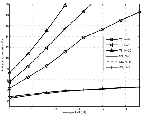
Figure 1: Performance comparison of different resource allocation schemes

Fig. 1 shows the simulated TAUR in the network by using the proposed TS policy and the existing GS policy. Here the utility of both policies is specified to have the form

$$U(r)=\ln\left(1+\frac{r}{A}\right),$$ (6)

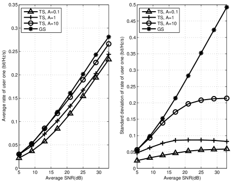
Figure 2: Average rate and standard deviation of rate versus average SNR using TS and GS

where $A>0$ is a concavity indicator. The channels are assumed to be Rayleigh fading and the SNR gap is set to $8.2$ dB for all users which corresponds to a bit-error-rate requirement of $10^{-5}$ when adaptive quadrature amplitude modulation (QAM) is used. The number of users in the network varies from 8 to 32 and their channel conditions are symmetric. The concavity indicator $A$ is set at $0.1$. Fig. 2 compares the mean and the standard deviation of the transmission rate achieved by TS and GS policies for $A=0.1,1$ and 10 with $N=32$. The performances of the GS policy at different values of $A$ are identical due to the channel symmetry among the users. In fact, it is an extreme case of our TS policy when $A\to\infty$ . Although GS can obtain the maximum average rate, the standard deviation of the rate increases rapidly as the average SNR increases. The TS policy, on the other hand, has a flexible balance between the average rate and the rate oscillation through adjusting the concavity of the utility function.

IV joint time-sharing and power control

In this section we allow both the transmission time and power to change with respect to channel conditions in each time frame. The optimization problem in Section III is extended to finding the joint optimal time-sharing and power control policy. Uplink and downlink transmission are considered separately due to different power constraints. For the uplink, the power source is, generally, rechargeable batteries attached to the mobile devices. Thus, the optimization is subject to each user’s average power constraint. Mathematically, this can be represented as

$$\max_{(\mbox{\boldmath$\rho$},\mathbf{p})} I_{\rm JTPC}\triangleq\int_{\mathbf{g}}\sum^{N}_{i=1}U_{i}(\rho_{i}(\mathbf{g}),p_{i}(\mathbf{g}),g_{i})f(\mathbf{g})\mbox{d}\mathbf{g}$$ (7)

$${\rm s.t.} \sum^{N}_{i=1}\rho_{i}(\mathbf{g})=1$$ (9)

$$\int_{\mathbf{g}}\rho_{i}(\mathbf{g})p_{i}(\mathbf{g})f(\mathbf{g})\mbox{d}\mathbf{g}=\bar{p}_{i},~{}i=1,2,\ldots,N,$$

where $\bar{p}_{i}$ is the average power constraint of user $i$.

Note that the utility function $U(\rho,p,g)$ is concave in $\rho$ and $p$ separately based on our assumption, but not in both $\rho$ and $p$. Moreover, the equality constraints in (9) are nonlinear. To make the problem more tractable, we define $s=p\rho$. It can be shown that $U(\rho,s,g)$ is concave in both $\rho$ and $s$ (since its Hessian matrix is negative semidefinite). The problem thus falls into the classic calculus of variations [6]. Applying the Euler-Lagrange equation results in the following necessary and sufficient conditions for the optimal solution $\rho_{i}^{*}$ and $s_{i}^{*}$:

$$\frac{\partial U_{i}}{\partial s_{i}}+\lambda_{i}=0,~{}~{}~{}i=1,2,\ldots,N$$ (10)

$$\frac{\partial U_{i}}{\partial\rho_{i}}f(\mathbf{g})+\lambda_{0}(\mathbf{g})=0,~{}~{}~{}i=1,2,\ldots,N$$ (11)

where $\lambda_{0}(\mathbf{g})$ and $\lambda_{i}$ are Lagrange multipliers and determined by constraints (9) and (9). The closed-form solutions to the above equations are generally difficult to obtain due to nonlinearity of the utility function $U$ in $\rho$ and $s$. The nonlinear Gauss-Seidel algorithm [7] can be used to search for the optimal time-sharing vector $\mbox{\boldmath$\rho$}^{*}$ and vector $\mathbf{s}^{*}=[s_{1}^{*},s_{2}^{*},\ldots,s_{N}^{*}]$ under the average power constraint $\mathbf{\bar{p}}=[\bar{p}_{1},\bar{p}_{2},\ldots,\bar{p}_{N}]$. It is outlined as follows.

1. Initialize $\mathbf{s}$: set $\mathbf{p}^{(0)}=N\mathbf{\bar{p}}$, $\rho_{i}=1/N$, $\forall i$, let $j=0$ and calculate the initial $\mathbf{s^{(0)}}$.

2. Update $\mathbf{\rho}^{(j)}$ : given $\mathbf{s}^{(j)}$, find the optimal time-sharing vector $\mbox{\boldmath$\rho$}^{(j)}$ using (11)

   $$\rho_{i}^{(j)}(\mathbf{g})=\left[\left(\frac{\partial U_{i}}{\partial\rho_{i}}\right)^{-1}\left(\lambda_{0}^{\prime},s^{(j)}_{i}\right)\right]^{+},~{}~{}i=1,2,\ldots,N,$$

   where $\lambda_{0}^{\prime}$ satisfies (9)

3. Compute the average aggregate utility $I^{(j)}$ using (7)

4. Update $\mathbf{s}^{(j+1)}$: given $\mbox{\boldmath$\rho$}^{(j)}$, find the optimal power control vector $\mathbf{s}^{(j+1)}$ using (10)

   $$s_{i}^{(j+1)}(\mathbf{g})=\left[\left(\frac{\partial U_{i}}{\partial s_{i}}\right)^{-1}\left(\lambda_{i},\rho^{(j)}_{i}\right)\right]^{+}~{}\mbox{for}~{}i=1,2,\ldots,N,$$

   where $\lambda_{i}$ satisfies (9) for $i=1,2,\ldots,N$ and let $j=j+1$.

5. Repeat Steps 2)-4) until $I^{(j+1)}-I^{(j)}<\Delta$, where $\Delta$ is a small number.

At each iteration, the optimization of $\rho$ and $\mathbf{s}$ is carried out successively. Steps 2) and 4) involve only the calculation of a one-dimensional maximization problem whose solution is given in Section III. The condition that $U$ is continuously differentiable and concave in ($\rho$, $s$) guarantees the convergence of the nonlinear Gauss-Seidel algorithm. The proof can be seen in [7, Prop 3.9 in Section 3.3].

The problem formulation for the downlink differs from the uplink only in the power constraint, which is given by $\int_{\mathbf{g}}\sum^{N}_{i=1}\rho_{i}(\mathbf{g})p_{i}(\mathbf{g})f(\mathbf{g})\mbox{d}\mathbf{g}=\bar{p}$. A similar problem-solving approach to the one proposed for the uplink can also be obtained and hence is omitted.

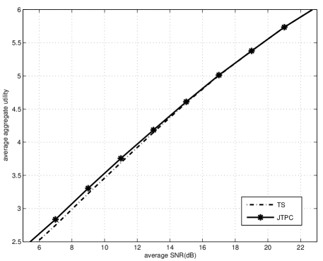
Figure 3: Average aggregate utility versus average SNR using TS and JTPA for two-user scenario

Although JTPC utilizes two degrees of freedom in resource allocation and has much higher computational complexity, its performance is not expected much higher than that of TS in the high SNR region. This is attributed to the fact that the transmission rate is linear in time, but concave in transmission power. That is, at high SNR, the gain from power control is smaller than from time sharing adaptation. This is also verified by the simulation results shown in Fig. 3, where we compare the average aggregate utilities obtained by the proposed TS and JTPC schemes. It is observed that at high SNR the performance gain of JTPC over TS is not noticeable. Hence, in Section V, we assume the absence of power control.

V Implementation Issues

We have provided the analytical results for TS and JTPC policies. In this section, we address some important implementation issues, including quantized time sharing fractions, limited channel feedback, and fairness.

V-A Quantized Time Sharing With Limited Channel Feedback

In scheduling the downlink transmission, the BS needs to know each user’s channel state information (CSI). This could be gained by sending the CSI from each user to the base station through a feedback channel upon channel estimation at each user terminal. In practice, perfect channel feedback is not feasible due to limited capacity of the feedback links. We assume in this subsection that the channel estimate of each user is quantized into $K=2^{M}$ regions using $M$ bits. Let $\mathbb{G}=\{G_{1},G_{2},\ldots,G_{K+1}\}$ be the set of channel gain thresholds in increasing order with $G_{1}=0$ and $G_{K+1}=\infty$. If the channel gain of user $i$ falls into range $[G_{k},G_{k+1})$, we say user $i$ is in channel state $k$, and denote it as $S_{i}=k$. Suppose we apply the equal-probability method to do the channel partitioning and the channel gains follow exponential distribution, the threshold set $\mathbb{G}$ can be determined easily.

Furthermore, time sharing fractions in practice cannot be an arbitrary number, but are restricted to a finite set of values due to switching latency and difficulties in rigid synchronization. Therefore, we assume that a time frame is partitioned into $L$ slots with equal length. Correspondingly, the number of users which can transmit in the same frame is limited by $L$. At the beginning of each frame, the base station computes the optimal time-sharing vector $\mbox{\boldmath$\rho$}^{*}$ defined in (12) upon obtaining the network channel states $\mathbf{S}=[S_{1},S_{2},\ldots,S_{N}]$.

$$\mbox{\boldmath$\rho$}^{*}(\mathbf{S}) = \mbox{arg}\max_{\mbox{\boldmath$\rho$}(\mathbf{S})}~{}\int_{G_{S_{1}}}^{G_{S_{1}+1}}\int_{G_{S_{2}}}^{G_{S_{2}+1}}\ldots\int_{G_{S_{N}}}^{G_{S_{N}+1}}\left[\sum_{i=1}^{N}U_{i}(\rho_{i}(\mathbf{g}),g_{i})\right]\mbox{d}\mathbf{g}$$ (12)

s.t. $$\rho_{i}\in\left\{0,\frac{1}{L},\frac{2}{L},\ldots,1\right\},~{}\forall i\in\{1,\ldots,N\}~{}\mbox{and}~{}\sum_{i=1}^{N}\rho_{i}=1.$$

The time sharing policy considered here maps the current channel states $\mathbf{S}\in\mathbb{R}_{+}^{N}$ to a time-sharing vector To avoid the exponential complexity in exhaustive search, an online greedy algorithm with complexity of $\mathcal{O}(LN)$ is proposed. Beginning with an initial solution $\mbox{\boldmath$\rho$}=[0,0,\ldots,0]$, each time slot is assigned at one iteration to the most favorable user that maximizes the increment of the current objective till the total $L$ slots are traversed. The greedy algorithm is outlined below:

1. Initialization
   Let $v=0$ (the index of the time slot), $\rho_{i}^{(0)}=0$ and $U_{i}^{(0)}=0~{}(\forall i\in\{1,\ldots,N\})$.

2. Allocate the $(v+1)^{th}$ time slot to the user indexed by ${i}^{*}$

   $$i^{*}=\mbox{arg}~{}\max_{i\in\{1,\ldots,N\}}~{}\int_{G_{S_{i}}}^{G_{S_{i}+1}}\bigg{[}U_{i}(\rho_{i}^{(v)}+1/L)-U_{i}(\rho_{i}^{(v)})\bigg{]}\mbox{d}{g_{i}}.$$ (13)

   Let $\rho_{i^{*}}^{(v+1)}=\rho_{i^{*}}^{(v)}+1/L$ and $\rho_{i}^{(v+1)}=\rho_{i}^{(v)}$ for $i\neq i^{*}$.

3. Let $v=v+1$, and return to Step 2) until $v=L$

It is shown in the appendix that this algorithm leads to the optimal solution to Problem (12).

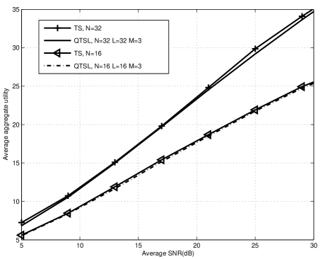
Figure 4: Performance comparison of the optimal TS policy and QTSL policy for $N=32$ and 16 users, with $L=N$ slots and $M=3$ feedback bits

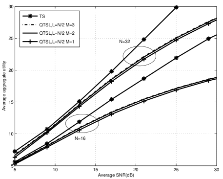
Figure 5: Performance comparison of $N=32$ users with $L=16$ and $N=16$ users with $L=8$ time slots, and with $M=1,2$ and 3 feedback bits

Fig. 4 shows the performance of the quantized time sharing with limited channel feedback (QTSL) policy. The CSI is quantized at 3-bit resolution, and the number of time slots is the same as the number of users in the network. It is seen that the performance of QTSL approaches that obtained by the optimal TS policy. In Fig. 5, we illustrate the performance of the QTSL policy when the number of time slots in a time frame is half of the number of users in the network. This time we also vary the number of channel feedback bits from $1$ to $3$. There is a performance gap between QTSL and TS, but the average aggregate utility obtained by QTSL with $N=32$ and $L=16$ is still higher than that of the optimal TS policy with $N=16$. In addition, the performance gain is limited when the CSI is quantized using more than two bits.

V-B Fairness Guarantee

The scheduling schemes based on the aggregate utility maximization developed in previous sections may not guarantee fairness for users with different channel statistics, such as path loss and shadowing. This is because the TS scheme tends to allocate more time to the user with higher average SNR. A commonly used fairness criterion in computer networks is the max-min fairness [8]. Unlike wireline networks, the wireless network suffers from time-varying channel impairments. Thus, time-average utility max-min (TUMM) fairness, defined below, is meaningful in wireless networks.

Definition 1: A time sharing policy $\rho$ is time-average utility max-min fair if for each $i\in\{1,2,\ldots,N\}$ and any other time sharing policy $\bar{\mbox{\boldmath$\rho$}}$ for which $\mathbb{E}[U_{i}(\rho_{i})]<\mathbb{E}[U_{i}(\bar{\rho_{i}})]$, there exists some $j$ with $\mathbb{E}[U_{i}(\rho_{i})]\geq\mathbb{E}[U_{j}({\rho_{j}})]>\mathbb{E}[U_{j}(\bar{\rho}_{j})]$, i.e., increasing some component $\mathbb{E}(U_{i}(\rho_{i}))$ must be at the expense of decreasing some already smaller component $\mathbb{E}[U_{j}(\bar{\rho_{j}})]$

Since the resource allocation based on TUMM fairness does not concern the fairness at any instant, it allows the scheduler to exploit the instantaneous fluctuation of the channel conditions. We formulate the TUMM-based time sharing as a multiple-objective programming problem:

$$\max_{\mbox{\boldmath$\rho$}(\mathbf{g})} a$$ (14)

s.t. $$\mathbb{E}[U_{i}(\rho_{i}(\mathbf{g}),g_{i})]=a,~{}i=1,2,\ldots,N$$

$$\sum^{N}_{i=1}\rho_{i}(\mathbf{g})=1,$$

where $a$ is a variable to be maximized. When $U_{i}(\cdot)$’s are all strictly concave, there exists a unique solution.

A frequently used method in multiple objective programming problem is the point estimate weighted-sum approach [9]. In this method, each objective is multiplied by a weight $w_{i}$. Then, the $N$ weighted objectives are summed to form a weighted-sum objective function, denoted as $\sum^{N}_{i=1}w_{i}\mathbb{E}[U_{i}(\rho_{i})]$. The weights $w_{i}$’s are chosen such that (V-B) is satisfied. It can be proven that the solution to maximize the average aggregate weighted utility is also Pareto-optimal. Take the two-user case for example. The notion of fairness can be realized by dynamically adjusting the weights, i.e., dynamically adjusting the moving direction towards the intersection of the Pareto-optimal frontier and the straight line $\mathbb{E}[U_{1}]=\mathbb{E}[U_{2}]$ while keeping the two users’ average utility on the Pareto-optimal frontier. This weight adaptation method can be used to guarantee fairness when the users have different channel distributions.

VI Conclusion

We develop a new framework for resource allocation in wireless networks for variable-rate transmission. The time-average aggregate utility of instantaneous transmission rate is proposed to jointly optimize the resulting average rate and rate oscillation. In particular, a time-sharing policy and a joint time-sharing and power control policy are designed to exploit the channel fluctuation. The effects of partial channel state information and discrete time sharing fractions are also studied. Furthermore, an adaptive method to guarantee strict fairness among users with different channel statistics is discussed.

[Optimality Proof of The Greedy Algorithm] Consider one realization of $S$ and $\rho_{i}\in\{0,{1}/{L},{2}/{L},\ldots,1\}$. For simplicity, we define $\tilde{U}_{i}(\rho_{i}):=\int_{G_{S_{i}}}^{G_{S_{i}+1}}U_{i}(\rho_{i}(\mathbf{g}),g_{i})\mbox{d}{g_{i}}$ and $d_{i}(\rho)=\tilde{U}_{i}(\rho)-\tilde{U}_{i}\left(\rho-{1}/{L}\right)$. Let $D_{L}$ denote the set of $L$ largest elements in $D=\{d_{i}(\rho)|i=1,2,\ldots,N,\rho=0,1/L,2/L,\ldots 1\}.$ Then, the Lagrangian can be written as:

$$\sum_{i=1}^{N}(\tilde{U}_{i}(\rho_{i})-\lambda\rho_{i})=\sum_{i=1}^{N}[\tilde{U}_{i}(0)+(d_{i}(1/L)-\lambda)+\ldots+(d_{i}(\rho_{i})-\lambda)].$$ (16)

Let $\lambda$ be the smallest $d_{i}(\rho)$ in $D_{L}$, then

$$d_{i}(\rho)-\lambda\left\{\begin{array}[]{ll}\geq 0&\mbox{if}~{}d_{i}(\rho)\in D_{L}\\ <0&\textrm{otherwise}\end{array}\right..$$ (19)

Therefore the Lagrangian (16) is maximized by

$$\rho_{i}^{*}=\left\{\begin{array}[]{ll}0&\mbox{if}~{}d_{i}(1/L)\notin D_{L}\\ 1&\mbox{if}~{}d_{i}(1)\in D_{L}\\ \rho&\mbox{if}~{}d_{i}(\rho)\in D_{L}~{}\mbox{and}~{}d_{i}(\rho+1/L)\notin D_{L}.\end{array}\right..$$ (23)

Due to the concavity of the utility function, we have $d_{i}(1/L)>d_{i}(2/L)>\ldots>d_{i}(N_{i}/L)>d_{i}((N_{i}+1)/L)>\ldots>d_{i}(1)$. Here suppose that $d_{i}(N_{i}/L)\in D_{L}$ and $d_{i}((N_{i}+1)/L)\notin D_{L}$, then $\sum_{i}N_{i}=|D_{L}|$. Since $\rho_{i}^{*}=N_{i}/L$ from (23), $\sum_{i}\rho_{i}^{*}=|D_{L}|/L=1$ holds for the chosen $\lambda$. $\rho_{i}^{*}$ is an optimal solution of Problem (12).

Since Step 2) computes the $L$ largest $d_{i}(\rho)$ in the decreasing order of their values, the greedy algorithm obtains the optimal solution.

References

- [1] P. Viswanath, D. Tse, and R. Laroia, “Opportunistic beamforming using dumb antennas,” IEEE Trans. on Info. Theory, vol. 48, no. 6, pp. 1277–1294, June 2002.
- [2] A. Jalali, R. Padovani, and R. Pankaj, “Data throughput of cdma-hdr a high efficiency-high data rate personal communication wireless system,” in Proc. Veh. Technol. (VTC), 2000.
- [3] A. L. Stolyar, “On the asymptotic optimality of the gradient scheduling algorithm for multiuser throughput allocation,” Operation Research, vol. 53, no. 1, pp. 12–25, Jan. 2005.
- [4] X. Qiu and K. Chawla, “On the performance of adaptive modulation in cellular systems,” IEEE Trans. on Commun., vol. 47, no. 6, pp. 884–895, June 1999.
- [5] X. Zhang, M. Tao, and C. S. Ng, “Time sharing policy in wireless networks for variable rate transmission,” in Proc. IEEE ICC 2007, June 2007.
- [6] B. S. Gottfried and J. Weisman, Introduction to optimization theory. Prentice-Hall, 1973.
- [7] D. P. Bertsekas and J. N. Tsitsiklis, Parallel and Distributed Computation: Numerical Methods. Athena Scientific, 1997.
- [8] J. M. Jaffe, “Bottleneck flow control,” IEEE Trans. Commun., vol. 29, no. 7, pp. 954–962, July 1981.
- [9] R. E. Steuer, Multiple Criteria Optimization: Theory, Computation, and Application. Wiley, New York, 1986.