Crime and punishment: the economic burden of impunity

Abstract

Crime is an economically important activity, sometimes called the “industry of crime”. It may represent a mechanism of wealth distribution but also a social and economic charge because of the cost of the law enforcement system. Sometimes it may be less costly for the society to allow for some level of criminality. A drawback of such policy may lead to a high increase of criminal activity that may become hard to reduce. We investigate the level of law enforcement required to keep crime within acceptable limits and show that a sharp phase transition is observed as a function of the probability of punishment. We also analyze the growth of the economy, the inequality in the wealth distribution (the Gini coefficient) and other relevant quantities under different scenarios of criminal activity and probability of apprehension.

1 Introduction

Crime is a human activity probably older than the crudely called “oldest profession”. Criminal activity may have many different causes: envy, like in the case of Cain and Abel genesis , jealousy like in the opera Carmen, or financial gain like Jacob cheating Esau with the lentil pottage (and his father with the lamb skin) to obtain the birthright genesis2 . This is to say that crime can have many different causes, some of them “passional”, sometimes “logical” or “rational” VolterraConsulting03 .

All along history, organized societies have tried to prevent and to deter criminality through some kind of punishment. In all the societies and all the times punishment has been in some way proportional to the gravity of the offense. Methods ranged from the lex talionis “an eye for an eye”, to fines, imprisonment, and the death penalty. Most of the literature on crime considered criminals as deviant individuals. Usual explanations of why people offend use concepts like insanity, depravity, anomia, etc. In 18th Century England criminals were massively “exported” to Australia because it was thought that the criminal condition was hereditary and incurable: incapacitation was the solution.

In any case the increase of criminal activity in different countries have led some sectors of the population, as well as politicians, to ask for harder penalties. The understated idea is that a hard sentence, besides incapacitation of convicted criminals, would have a deterrent effect on other possible offenders and would also prevent recidivism. Yet, the deterrent effect of punishment is a polemic subject and law experts diverge with respect to whether offenders should be rehabilitated or simply punished (see for example the recent public discussion in France Salas06 ). In many countries, incapacitation is the main reason for imprisonment of criminals. For instance the Argentinean constitution states that prisons are not there for the punishment of the inmates but for the security of the society: criminals are isolated, not punished argent .

Although the idea that the decision of committing a crime results from a trade off between the expected profit and the risk of punishment dates back to the eighteen and nineteenth centuries, it is only recently that crime modeling emerged as a field worth of being investigated.

In a review paper, Alfred Blumstein Blumstein02 traces back the recent interest in crime modeling to 1966, when the USA President’s Commission on Law Enforcement and Administration of Justice created a Task Force on Science and Technology. Composed mainly by engineers and scientists, its aim was to introduce simulation modeling of the American criminal justice system. The model allowed to evaluate the resource requirements and costs associated to a criminal case, from arrest to release, by considering the flow through the justice system. For example, it estimated the opportunity of incarceration of convicted criminals and the length of the incarceration time. In his concluding remarks, Blumstein states that: “We are still not fully clear on the degree to which the deterrent and incapacitation effects of incarceration are greater than any criminalization effects of the incarceration, and who in particular can be expected to have their (tendency to) crime reduced and who might be made worse by the punishment”.

In a now classical article G. Becker Becker68 presents for the first time an economic analysis of costs and benefits of crime, with the aim of developing optimal policies to combat illegal behavior. Considering the social loss from offenses, which depends on their number and on the produced harm, the cost of aprehension and conviction and the probability of punishment per offense, the model tries to determine how many offenses should be permitted and how many offenders should go unpunished, through minimization of the social loss function.

Using a similar point of view, Ehrlich Ehrlich75 ; Ehrlich96 develops an economic theory to explain participation in illegitimate activities. He assumes that a person’s decision to participate in an illegal activity is motivated by the relation between cost and gain, or risks and benefits, arising from such activity. The model seemed to provide strong empirical evidence of the deterrent effectiveness of sanctions. However, according to Blumstein Blumstein02 the results “… were sufficiently complex that the U.S. Justice Department called on the National Academy of Sciences to convene a panel to assess the validity of the Erlich results. The report of that panel highlighted the sensitivity of these econometric models to details of the model specification, to the particular time series of the data used, and to the sensitivity of the instrumental variable used for identification, and so called into question the validity of the results”. In fact, the issue of what constitutes an optimal crime control policy is still controversial.

Another controversial subject is the relationship between raising of income inequality and victimization. Becker’s economic model of crime would suggest that as income distribution becomes wider, the richer become increasingly attractive targets to the poorer. There are many reasons why this hypothesis may not be correct. For example, Deutsch et al. DeutschSpiegelTempleman92 consider the impact of wealth distribution on crime frequency and, contrary to the general consensus in the literature, conclude that variations of the wealth differences between “rich” and “poor” do not explain variations in the rates of crime. Bourguignon et al BourguignonNunezSanchez02 based on data from seven Colombian cities conclude that in crime modeling the average income of the population determines the expected gain, but that potential criminals belong to the segment of the population whose income is below $80\%$ of the mean. More recently, Dahlberg and Gustavsson DahlbergGustavsson05 pointed out that in crime statistics one should distinguish between permanent and transitory incomes. Disentangling these income components based on tax reports in Sweden, they find that an increase in inequality in permanent income (measured through the variance of the distribution) yields a positive and significant effect on crime rates, while an increase in the inequality due to a transitory income has no significant effect. Levitt Levitt99 concludes from empirical data that, probably because rich people engage in behavior that reduces their victimization, the trends between 1970 and 1990 is that property crime victimization has become increasingly concentrated on the poor.

As pointed out by many authors, the fact that police reduces crime is far from being demonstrated. Realizing that (at least in the U.S.A.) the number of police officers increases mostly in election years, Levitt Levitt97 has studied the correlation between these variations (uncorrelated to crime) and variations in crime reduction. He finds that increases in the size of police forces substantially reduce violent crime, but have a smaller impact on property crime. Moreover, the social benefit of reducing crime is not larger than the cost of hiring additional police. Similar conclusions have been drawn by Freeman FreemanRB96 , who estimates that the overall cost of crime in the US is of the order of 4 percent of the GDP, 2 per cent lost to crime and 2 percent spent on controlling crime. This amounts to an average of about $54,000$ dollars/year for each of the 5 million or so men incarcerated, put on probation or paroled.

In most models, punishment of crime has two distinct aspects: on one side there is the frequency at which illegal actions are punished (which corresponds to the punishment probability in the models), and on the other, the severity of the punishment. In a review paper, Eide Eide99 comments that although many empirical studies conclude that the probability of punishment has a preventive effect on crime, the results are ambiguous.

More recent reviews of the research literature consider the factors influencing crime trends VolterraMarris00 and present some recent modeling of crime and offending in England and Wales VolterraConsulting03 . They both note the above mentioned difficulties in estimating the parameters of the models and the cost of crime.

Most of the models in the literature follow Becker’s economic approach. Ehrlich Ehrlich96 presents a market model of crime assuming that individuals decisions are “rational”: a person commits an offense if his expected utility exceeds the utility he could get with legal activities. At the “equilibrium” between the supply of crimes and the “demand” (or tolerance) to crime — reflected by the expenditures for protection and law enforcement – neither criminals, private individuals nor government can expect to improve their benefits by changing their behaviors. In particular, the model is based on standard assumptions in economic models, with “well behaved” monotonic supply and demand curves, which cannot explain situations where social interactions are important NaPhGoVa05 ; GoNaPhSe07 . Indeed, Glaeser et al GlaeserSacerdoteScheinkman96 attribute to social interactions the large variance in crime on different cities of the US.

Another kind of models CampbellOrmerod00 ; VolterraConsulting03 treat criminality as an epidemics problem, which spreads over the population due to contact of would-be criminals with “true” criminals (who have already committed crime). This kind of models incorporates effects due to social interactions, which introduce large nonlinearities in the level of crime associated to different combinations of the parameters. These may explain the wide differences reported in the empirical literature.

In this paper we focus on economic crimes, where the criminal agents try to obtain an economic advantage by means of the accomplished felony. No physical aggression or death of the victim will be considered, and on the side of punishment we consider the standard of most developed civilized countries, i.e. fines and imprisonment. We assume that web_dando “most criminal acts are not undertaken by deviant psychopathic individuals, but are more likely to be carried out by ordinary people reacting to a particular situation with a unique economic, social, environmental, cultural, spatial and temporal context. It is these reactionary responses to the opportunities for crime which attract more and more people to become involved in criminal activities rather than entrenched delinquency”.

We simulate a population of heterogeneous individuals. They earn different wages, have different tastes for criminality, and modify their behaviors according to the risk of punishment. We assume that both the probability and the severity of the punishment increase with the magnitude of the crime. We are interested in the consequences of the punishment policy on the costs of crime, in the wealth distribution consistent with different levels of criminality, in the economic growth of the society as a function of time, and in the (possibly bad) consequences of allowing for some criminal activity in order to minimize the cost of the law enforcement apparatus. In section 2 we describe the model, in section 3 we explain its dynamics. We present the results of the simulations in 4 and leave the conclusions to section 5

2 Description of the model

We consider a model of society with a constant number of agents, $N$, who perceive a periodic (monthly) positive income $W_{i}$ (that we call wage), spend part of it each month and earns the rest. Wages remain constant during the simulated period. In our simulations, the wages distribution has a finite support: $W_{i}\in[W_{min},W_{max}]$. In this utopian society there is not unemployment, and it is assumed that the minimum wage is enough to provide for the minimum needs of each agent, i.e. a person perceiving the minimum wage will expend it completely within the month. These wages and possibly the booties of successfully realized crimes constitute the only income source of the individuals. Besides the living expenses, capitals may decrease due to plunders and to the taxes or fines related to conviction, as explained later.

We assume that each agent has an inclination to abide by the law, that is represented by a honesty index $H_{i}$ ($i\in[1,N]$) which, at the beginning of the simulations ranges between a minimum and a maximum: $H_{i}\in[H_{min},H_{max}]$. This inclination — that may be psychological, ethical, or reflect educational level and/or socio-economical environment — is not an intrinsic characteristic of the individuals. It changes from month to month according to the risk of apprehension upon performing a crime.

In our simulations, the individual decision of committing a crime depends (not exclusively) on both the honesty index and the monthly income, which are initially drawn at random from distributions $p_{H}$ and $p_{W}$ respectively, without any correlation among them. This is justified by the lack of empirical evidence that the poorer are more or less law abiders than the rich.

The honesty index of all the individuals but the criminal increases by a small amount each time a crime is punished. Otherwise it decreases, but at a different rate for the criminal than for the rest of the population. The honesty index is not affected by the importance of the punishment. This assumption is an extreme simplification of the observation Blumstein02 that the crime rate is more sensitive to the risk of apprehension than to the severity of punishment. We have studied different distributions $p_{H}$ and $p_{W}$ and different treatments of the honesty index. The latter differ in the way we treat the lower bound of the distribution $p_{H}$, namely $H_{min}$. Hereafter we describe in details the simplest case: we consider that $H_{min}$ is an absolute minimum of the honesty. $H_{min}$ corresponds thus to the honesty index of the most recalcitrant offenders. But we also add the hypothesis (that is certainly controversial) that for those agents with this lowest honesty there is no possible redemption, i.e. when the honesty index of an agent decreases down to $H_{min}$ it remains there for ever. We leave to forthcoming discussions the possible variations of this scheme.

As a consequence of this treatment, there are intrinsic criminals (those with $H_{i}=H_{min}$). Indeed, a finite fraction, $N_{C}(0)$, of intrinsically criminal agents is assumed from the very beginning of the simulation, according with the idea that there always have been and will be a finite number of not redemptible criminals in a society. All the $N-N_{C}(0)$ other agents are “susceptible”: their degree of honesty $H_{i}(0)$, drawn at random from the probability distribution $p_{H}$, satisfies $H_{min}<H_{i}(0)\leq H_{max}$.

Individuals have also “social” connections: encounters between criminals and victims may only occur between socially linked individuals. These connections are not meant to represent social closeness but rather the fact that those individuals share common daily trajectories or live in close neighborhoods, or meet each other just by chance. For simplicity, here we consider the latter situation: every individual may be connected to every other individual.

Notice that the nature of social interactions in our model is very different from the mimetic interactions considered by Glaeser et al GlaeserSacerdoteScheinkman96 , or the social pressure introduced by Campbell et al. CampbellOrmerod00 . We study just the case of individual crimes. No illicit criminal associations (“maffia”) nor collective victims (like in bank assaults) are going to be considered.

The characteristics of the simulated population evolve on time. We assume that every month there is a number of possible criminal attempts. This number depends on the honesty index of the population as is explained later. Among these attempts, some are successful, i.e. the criminal spoils his victim of a (random) fraction of his earnings.

In contrast with most models, crimes are punished with a probability that depends on the magnitude of the loot. When punished, the criminal returns part of the booty to the victim, pays a fine that may be considered as a contribution to the public enforcement system and goes to jail for a number of months that also depends on the stolen amount. Maintaining each criminal in prison bears a fixed cost per month to the society, that we evaluate.

In our simulations we study the month to month evolution of different quantities that characterize the system, and how these depend on the probability of punishment.

3 Monthly dynamics

Starting from initial conditions of honesty, wages and earnings described in section 3.1, we simulate the model for a fixed number of months. Within each month, there is a random number of criminal attempts correlated with the honesty level of the population (section 3.2). However, not all the attempts end up with a crime: the potential criminal has to satisfy some reasonable conditions that we explicit in section 3.3. If there is crime, there is a transfer of the stolen value from the victim to the criminal, as detailed in section 3.4. Some of the offenders are detected and punished (section 3.5): part of the stolen amount is then returned to the victim and a fine or tax is levied from the criminal’s earnings. In turn, the honesty of the population evolves after each crime, according to the success or failure in crime repression (section 3.6).

We keep track of the individuals’ wealth, taking into account the monthly incomes, the living expenses, the plunders, and the cost of imprisonment, as detailed in section 3.7.

In the following paragraphs we describe in details the dynamics of the model.

3.1 Initial conditions

The individuals have initial honesty indexes $H_{i}(0)$ and wages $W_{i}$ drawn with uncorrelated probability density functions (pdf) $p_{H}$ and $p_{W}$ respectively. We assume that the majority of the population is honest and also that the majority earn low salaries, i.e. $p_{H}$ has a maximum at large $H$ while $p_{W}$ has its maximum at small $W$. The results described below have been obtained considering triangular distributions, because they are the simplest way of introducing the desired individual inhomogeneities. Thus, $p_{W}$ is a triangular distribution of wages, with $W_{min}=1$ and $W_{max}=100$ (in some arbitrary monetary unit), with its maximum at $W_{min}$ and a mean value $\overline{W}=W_{min}+(W_{max}-W_{min})/3$. As already explained, there is an initial number of “intrinsic” criminals $N_{C}(0)$ drawn at random, with $H_{i}=H_{min}$. In our simulations this number has been set to $5\%$ of the population ($N_{C}(0)=0.05N$). The honesty index of the remaining (susceptible) individuals is triangular, from $H_{min}=0$ up to $H_{max}=100$, with the maximum at $H_{max}$.

Individuals’ initial endowments are arbitrarily set to five months wages: $K_{i}(0)=5\,W_{i}$. This initial amount controls the time needed for the dynamics to fully develop. Smaller initial endowments result in transients dominated by the size of the possible loots, because these cannot exceed the victims’ capitals.

3.2 Attempts

The number of criminal attempts each month $m$ is $A(m)=[{\cal A}(m)]$ where $[\dots]$ represents the integer part, and

$${\cal A}(m)=\left\{\begin{array}[]{lll}1+r(m)\,c_{A}\,N+&\frac{H_{max}(m)-\overline{H}(m)}{\overline{H}(m)}\ N_{C}(m)&\\ &{\rm if}\overline{H}(m)\neq H_{min}&,\\ \\ 1+r(m)\,c_{A}\,N+&2\,N_{C}(m)&\\ &{\rm if}\overline{H}(m)=H_{min}&.\end{array}\right.$$ (1)

$r(m)\in[0,1]$ is a random number drawn afresh each month, $0<c_{A}<1$ is a coefficient (in the simulations $c_{A}=0.01$) and $N_{C}(m)$ are the number of intrinsic offenders (who have $H_{i}=0$) at month $m$. With these considerations there is always a ground level of criminal attempts given by the term proportional to $N$. Criminality increases with the number of intrinsic offenders and with a decreasing average honesty. When the latter equals $H_{min}$ all the population has the minimum of honesty, i.e. everybody is an “intrinsic” offender. In this case, to avoid the divergence in the first of equations (1), the prefactor of $N_{C}$ was set arbitrarily to $2$.

At each criminal attempt a potential offender is selected as explained in subsection 3.3 and the number of remaining attempts for the month is decreased by one, even if the crime is aborted.

3.3 Criminals

We consider that the possible criminals have low honesty indexes, and that it is more likely that they have low wages. Then, at each attempt, a potential criminal $k$ is drawn at random among the population of free (not imprisoned) individuals (we discuss in 3.5 when and how long punished offenders go in jail). We also select at random an upper bound $H_{U}$ to the honesty index in the interval $[H_{min},H_{max}]$. If

$$H_{k}<H_{U},$$ (2)

then the offense takes place with a probability:

$$p_{k}=e^{-W_{k}/\overline{W}},$$ (3)

that is higher the lower the potential criminal wages. Thus, we select a random number in $[0,1)$. If it is larger than $p_{k}$, the criminal attempt is aborted.

3.4 Crime

If crime is actually committed, a victim $v$ among the social neighbors (not in jail) of $k$ is selected at random. We do not take into account the wealth of the victim, which may be an important incentive for the criminal’s decision. Thus, our treatment may be adequate for minor larcenies, like stealing in public transportation. In the crimes considered in this paper, the victim is robbed of a random amount $S$ that cannot be larger than his actual capital. In the simulation, this amount is proportional to the victim’s wage:

$$S=r_{S}\,c_{S}\,W_{v},$$ (4)

where $r_{S}\in[0,1]$ is a random number drawn afresh at each attempt and $c_{S}>0$ is a coefficient (here we use $c_{S}=10$, implying that robbery may concern amounts up to 10 times the victim’s wage). If the value given by (4) is larger than the victim’s capital $K_{v}$, we set $S=K_{v}$. Correspondingly, the victim’s capital is decreased by the stolen amount, to become $K_{v}-S$ while the criminal’s capital is in turn increased to $K_{k}+S$.

3.5 Punishment

The criminal may be catched and punished with probability

$$\pi(S)=\frac{p_{1}}{1+\frac{p_{1}-p_{0}}{p_{0}}e^{-\frac{S}{\overline{K}(m)}}},$$ (5)

a monotonic function that starts at its minimal value $p_{0}$ (for $S=0$ ), increases almost linearly with $S$ for values of $S$ smaller than $\approx\overline{K}(m)$, the population’s average wealth, and gets close to the asymptotic value $p_{1}$ for large booties.

A punished criminal is imprisoned for a number of months $1+[S/\overline{W}]$ (the square brackets mean integer part), i.e. proportional to the stolen amount. During this time he does not earn his monthly wage and cannot be selected as a potential offender nor as a victim.

Beyond incarceration, the convicted criminal suffers a financial loss. He is deprived of an amount $(f_{R}+f_{D})S$, larger than the loot but that cannot exceed his total wealth (we do not allow for negative capitals). It is worth to remark that the financial loss is not limited to reimburse the stolen capital. A monetary punishment (a fine) is inflicted to the offender together with the time in prison (that represents, in addition to be incarcerated, also a monetary loss). The total amount deduced from the offender’s capital is composed of a fraction $f_{R}S$ (with $f_{R}<1$), that is returned to the victim, and an amount, $f_{D}S$ (or $K_{k}-f_{R}S$ if $f_{D}S>K_{k}$), considered as a duty. Cumulated duties or “taxes” constitute the total income of fines. In this simulation $f_{R}=0.75$ and $f_{D}=0.45$, meaning that both criminals and victims contribute to taxes, since the victims only recover a fraction $1-f_{R}$ of the stolen amount. However, with the assumed values of $f_{R}$ and $f_{D}$, $f_{R}+f_{D}=1.2$, implying that the criminals also afford part of the costs.

3.6 Honesty dynamics

We assume that punishment has a dissuasive effect on the population, although not necessarily on the convict. Thus, whenever a criminal is convicted, the honesty index of all the population but the criminal, is increased by a fixed amount $\delta H$. Convicted criminals do not change their honesty level. On the contrary, when the crime is not punished, the entire population but the criminal decrease their honesty index by $\delta H$, while the criminal decreases his by $2\delta H$: unpunished criminals become even less honest.

In the present simulations we do not allow $H_{i}$ to become negative. Moreover, the lower bound of the distribution is absorbing. Thus, individuals reaching $H_{i}=H_{min}$ have their honesty index freezed, and henceforth are considered as “intrinsic” criminals.

A dynamics with a non-absorbing bound for the honesty dynamics gives similar results to those presented here. A variant that we did not implement yet is to modify the honesty level of the criminal proportionally to the importance of the loot.

3.7 Monthly earnings and costs

At the end of each month $m$, after the $A(m)$ criminal attempts are completed, the individuals’ cumulated capitals $K_{i}(m)$ are updated: the total capital of each agent, $K_{i}(m)$, is increased with his salary and decreased with his monthly expenses. Notice that the criminals’ and the victims’ capitals have been further modified during the month, according to the results of the criminal attempts.

We assume that individuals need an amount $W_{min}+f\times(W_{i}-W_{min})$ with $f<1$ to cover their monthly expenses. Thus, individuals with higher wages spend a proportional part of their income in addition to the minimum wage $W_{min}$. This is a simplifying assumption which may be questionable since the richer the individuals, the smaller the fraction of income they need for living but, on the other hand, rich people spent more in luxury goods. Assuming a more involved model for the expenses would modify the monthly wealth distribution, making it more unequal, but we do not expect that the qualitative results of our simulations would be modified.

In order to quantify the expenditure of conviction and imprisonment, we assume that the monthly cost of maintaining a criminal in jail is equal to the minimal wage. This is clearly a too simple hypothesis, that does not take into account the fixed costs of maintaining the public enforcement against crime. It is just a mean of assessing some social cost proportional to the criminal activity. The cumulated taxes, obtained through punishment of convicted criminals are thus decreased by an amount $W_{min}$ per month for each convict in jail.

At the end of each month, the time that inmates have to remain in prison (excluding the criminals convicted during that month) is decreased by one; those having completed their arrest punishment are freed.

4 Simulation results

Starting with the initial conditions, there are $A(m)$ criminal attempts each month $m$ as described in the subsection 3.2. As a consequence of the criminal activity, during the month the capitals of criminals and victims are modified, as well as the honesty index of the population. With the above dynamics, the earnings and the honesty distributions are shifted and distorted. The system may even converge to a population where all the initially susceptible individuals end up as intrinsically criminal.

We simulated systems of $N=1\,000$ agents for a period of $240$ months, under different distributions of honesty and wages. Here we report results corresponding to the triangular distributions described in section 2: wages have a linearly decreasing distribution in $[W_{min},W_{max}]$ with $W_{min}=1$ and $W_{max}=100$: there are more individuals with low wages than with high ones. The honesty distribution is also triangular, but increasing: starting with $p_{H}(H_{min})=0$, it increases linearly reaching its maximum at $p_{H}(H_{max})$, which corresponds to assuming that there are more honest than dishonest individuals.

4.1 Evolution of criminality with time

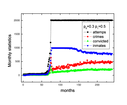
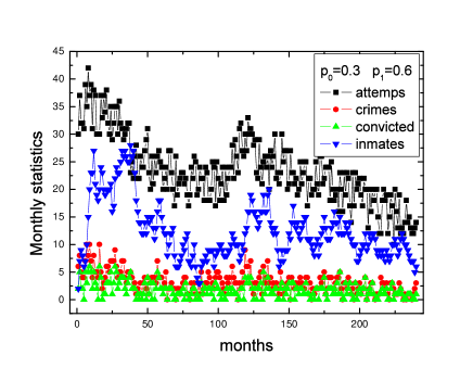
Figure 1: Statistics of criminality per month. Attempts: number of criminal attempts in the month. Crimes: number of crimes committed in the month. Convicted: number of criminals punished in the month. Inmates: number of criminals in jail. The difference between the left (a) and the right (b) panels is the maximum punishment probability $p_{1}$, $p_{1}=0.5$ in the left panel and $p_{1}=0.6$ in the right panel. Therefore, a small change in the probability of punishment induce a enormous change in the criminality (see the difference in scale in the ordinate axis).

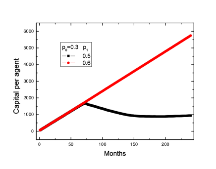
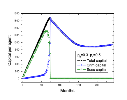
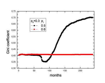
Figure 2: Capital and Gini monthly statistics: panel (a) shows the cumulated capital per agent as a function of time (the black curve corresponds to $p_{1}=0.5$ and the red one to $p_{1}=0.6$), panel (b) shows the participation in the total capital of intrinsic criminals (blue line) and susceptible ones (green line) just for the case of high criminality, $p_{1}=0.5$; panel (c) shows the Gini coefficient for two values of $p_{1}$, as in panel (a).

The system’s evolution is very sensitive to the punishment probability. Generally, the first months the rate of crime is low because the number of intrinsic criminals is small and the stolen amounts cannot be larger than the initial endowments. But after some months (the number depends on the initial conditions and on the values of $p_{0}$ and $p_{1}$) the crime rate increases to a stationary value.

Figure 1 shows a typical monthly evolution of the number of attempts, the number of crimes, the number of convicted criminals (which are the criminals punished in the corresponding month) and of inmates. The left figure corresponds to relatively low values of both $p_{0}$ (the probability of punishing small offenses) and $p_{1}$ (the probability of punishing large offenses) in (5). Beyond about $75$ months the number of attempts increases through an avalanche to reach its saturation value, while the number of inmates grows to reach almost all the population, producing a drop in crime. This drop is not due to a deterrent effect of punishment but rather to the absence of possible criminals (they are all in jail). Eventually the system evolves to a smaller number of inmates, but the population is essentially composed of individuals with the smallest honesty index: the punishment rate is not enough to keep criminality below any acceptable level. The figure on the right (see the change in the ordinate scale) corresponds to a slightly higher value of $p_{1}$, showing the impressive impact of increasing the probability of punishment of big offenses. All the quantities (attempts, crimes, etc.) present a dramatic decrease with respect to the values in the left hand side figure. Notice that the fluctuations on the reported quantities are of the same order of magnitude in both figures: they are due to the probabilistic nature of the quantities involved (see equations (1) to (5) ).

Correspondingly, the earned capital per individual (figure 2 upper left) increases almost linearly with time when crime is limited. In contrast, in the highly criminal society ($p_{1}=0.5$) it begins to decrease as soon as the regime of high criminality is reached, mainly because most criminals are convicted and do not receive their wages, but also because, since the number of punished crimes is also high, the amount retained in the form of taxes is discounted from the total wealth of the society. Moreover, the high cost of imprisonment, proportional to the total number of inmates, drains also part of the capital and contributes to decrease the capital per capita. This is illustrated on figure 2 upper right, where the total capital per agent is decomposed into the capital hold by the intrinsic criminals and the part hold by the susceptible population (with honesty index $H_{i}>0$). When the system reaches the high criminality regime the latter drops to zero because there are no more susceptible individuals. Clearly, when the level of punishment is not high enough to guarantee an effective control of criminality, the cost of the repressive system is very high. It is remarkable that a very small increase of the upper value $p_{1}$ in (5) is enough for a complete change in the scenario.

The lower figure 2 presents the evolution of the Gini index of the population, defined by:

$$G=\frac{\sum_{j=1}^{N-1}\sum_{i=j+1}^{N}|K_{i}-K_{j}|}{(N-1)\sum_{i}^{N}K_{i}}.$$ (6)

The Gini index spans in the interval $[0,1]$ and measures the inequality in the wealth distribution of the population. Its minimal value, $G=0$, corresponds to a perfectly equalitarian society. The Gini index of the initial endowment, distributed according with a triangular probability density, is $G(0)=0.4$. Due to the dynamics, when crime level is moderate ($p_{1}=0.6$) $G$ is seen to slightly increase. However, in the high criminality regime ($p_{1}=0.5$) it oscillates, and when the high crime rate sets in, it first plummets down because successful criminals, mostly individuals with small incomes according to the probability of crime (3), increase their wealths at the victims’ expense. As a result, the wealth distribution becomes more evenly distributed. However, on the long run, the Gini index increases dramatically. This is so because if everybody is a lawbreaker (lowest honesty index) criminals and victims are the same, just one stealing the other. So when one agent is in the victim role he becomes poor because of the robbery, and when he behaves as a crook he also finishes poor (generally), mainly because he pays taxes and also does not earn his wage when in jail. So, just a few agents are able to hold large capitals thanks to crime, increasing inequality in this society.

In fact, when $p_{0}$ is smaller than a critical value of the order of $0.5$, on increasing $p_{1}$, the system presents an abrupt transition between a high crime — low honesty population to a low crime — high honesty one. This transition, apparent on all the quantities, as may be seen below on figure 3, corresponds to a swing of the system between a regime of high criminality to one where the criminality level is moderately low.

In the high criminality side, cumulated earnings are small, taxes are high and the Gini index is large. Conversely, on the low criminality side, i.e. for sufficiently high $p_{1}$, the cumulated wealth increases monthly according to the earned wages, and the Gini index reflects the distribution of the latter. We will show in Figures 4, below, typical histograms of wealth distribution at both sides of the transition, as well as the initial distribution.

4.2 Changing the punishment probability

In the previous section we have discussed the time evolution of criminality. Let’s now consider the final state of the society (after 240 months) as a function of the probability of punishment. In order to make comparable experiments we have studied societies with the same initial conditions subjected to different levels of punishment. Notice that these levels are constant during the simulated 240 months.

We consider different values of $p_{0}$ smaller than a critical value of the order of $0.5$, and we study the variation of several social indicators as a function of $p_{1}$. We observe that the system ends up with either a high crime-low honesty population (for $p_{1}$ lower than a critical value) or a low crime-high honesty one. This transition, apparent on all the quantities, as may be seen on figures 3, corresponds to a swing of the system between a regime of high criminality to one of moderate criminality.

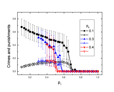
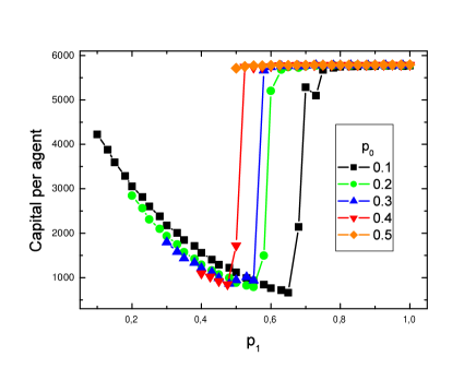
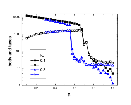
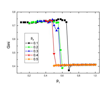
Figure 3: Panel (a): average number of crimes and convicted criminals over the simulated period. Panel (b): last month capital per capita of the population. Panel (c): average loot (full symbols) and taxes (empty symbols). Panel (d): last month Gini index.

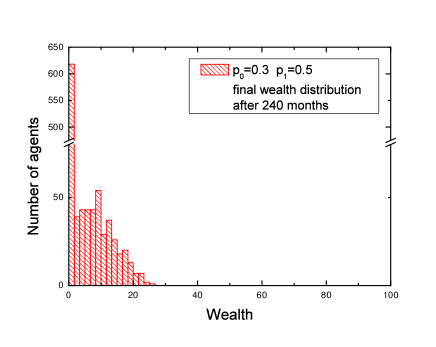
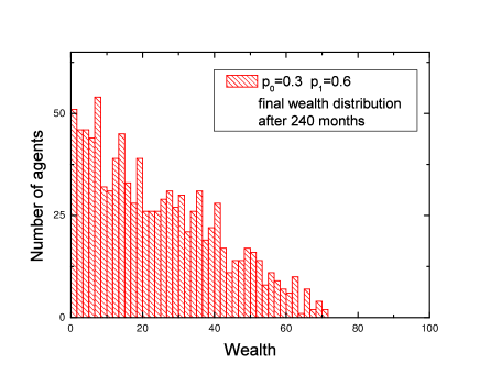
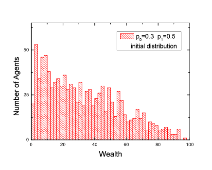
Figure 4: Histograms of the population wealth. Upper figures: at the end of the $240$ months with $p_{1}=0.5$ (a) and $p_{1}=0.6$ (b). Lower figure (c): initial state.

In the upper left panel of Figs. 3 the number of crimes and punishments per agent is represented for three representative values of $p_{0}$: $0.1$, $0.3$ and $0.4$. There is a sharp transition in the criminality when $p_{1}$ increases but the critical value strongly depends on the value of $p_{0}$. While for $p_{0}=0.4$ the transition happens for $p_{1}\simeq 0.52$, for $p_{0}=0.1$ the critical value grows up to $p_{1}=0.65$. This is an indication that the permissiveness in coping with small crimes have a deleterious effect, since the probability of punishment needed to deter important crimes increases.

A simple argument allows to understand the abrupt transition found in the simulations, which is correlated with a drop in the honesty level of the population. The average honesty level of the population increases roughly (we neglect the influence of criminal’s different dynamics) by about $\delta H$ if crimes are punished, and decreases by the same amount if not punished. Thus, we expect: $\bar{H}(m+1)\approx\bar{H}(m)+(1-\pi)\delta H-\pi\delta H$ per crime, where $\pi$ is the probability of the crime being punished. Clearly, there should be a change from an increasing honesty dynamics to a decresaing one for $\pi=1/2$. If crimes were punished with the same probability whatever the value of the loot ($p_{0}=p_{1}$), the change in the honesty dynamics would arise when this probability is equal to $1/2$. If small crimes have less probability of punishment, $p_{0}<1/2$, then $p_{1}$ must increase to keep the same dynamics on the average.

The upper right panel shows the total capital of the society. The effect of wrongdoing is evident. From a strictly economic point of view the worse situation arises closely below the critical point: a high level of criminal actions together with a relatively high frequency of punishment (although not enough to control criminality) have as a consequence a strong decrease in the total capital (because the cumulated effect of booties and taxes strongly reduces the total capital of the population). On the other hand, once the delinquency is under control the total capital of the society arrives to a maximum level.

The opposite effect is observed in the plot of the booties and taxes (left low panel). They are very high in the high criminality region (low values of $p_{1}$) and decrease strongly when $p_{1}$ is above its critical value.

Finally in the right low panel we have represented the Gini coefficient. If we observe this figure together with the evolution of the wealth of the society we can conclude that low criminality implies higher economic growth and less inequality. As the Gini coefficient is an average indicator, we present in Fig. 4 the wealth distribution histograms, in order to supply a complementary indicator. The two panels on top of Fig. 4 correspond to the histograms for the two values of $p_{0}$ and $p_{1}$ used on figures 1 and 2. It is clear that, for $p_{1}=0.5$, more than half of the agents have a vanishingly small capital, so explaining the high value of the Gini coefficient, while the total wealth of the population (represented by the total area of the histogram) is smaller that in the case of larger $p_{1}$. On the other hand, for $p_{1}=0.6$ the number of agents with wealth near zero falls down to $10\%$ of the population. Finally and just for comparison the lower figure represents the wealth distribution for the initial state (or, equivalently, the wages distribution).

We would like to emphasize that the results presented in this section are averages over $100$ independent samples at the end of $240$ months of evolution. We expect that modifying either $p_{0}$ or $p_{1}$ or both as a function of time (as it may happen in real societies in order to correct an abnormal increase of criminality) would produce different results because the initial conditions before the change in the probabilities are different (recall that here we assume a low initial number of low honesty agents). In fact if one starts in a state of high criminality, a very high probability of punishment (much higher than the critical values here presented) should be needed in order to reduce the criminality back to acceptable levels. Once more, preventive actions should be less expensive and easier to apply than trying to recover from a very deteriorated security situation.

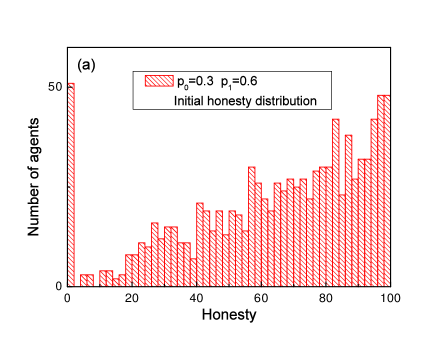
Figure 5: Histograms of the population’s honesty index. (a) initial distribution, where the small peak at zero honesty corresponds to the initial $5\%$ concentration of intrinsic criminals. (b) final distribution for $p_{0}=0.3$ and $p_{1}=0.6$: more than half of the population exhibits a honesty index $\geq 100$ while the number of intrinsic criminals remains the initial one. For $p_{0}=0.3$ and $p_{1}=0.5$ the honesty index of all the agents drops down to zero (and for this reason the plot is not included): a small change in the probability of punishment clearly induces a big change in the average honesty of the population.

5 Discussion and conclusion

A central hypothesis of our model is that the honesty level of the population is correlated with the mere existence (or absence) of punishment, but not with its importance (which is proportional to the size of the loot). Thus, punishing small crimes is as effective as punishing large ones for increasing the population’s honesty globally: the honesty level increases when crimes are punished and, on the contrary, impunity decreases it. Since small larcenies have a lower probability of being punished than large loots, the public effort on crime deterrence depends on the importance of the crime through the probability of punishment.

In Fig. 5 we represented the honesty distribution for the case $p_{0}=0.3$ and $p_{1}=0.6$ (panel (b)) and, for comparison, the initial distribution (panel (a)). We have not represented the case $p_{1}=0.5$ because in that case the honesty index of the entire population drops to zero, as discussed above: $p_{1}$ is not large enough and the criminality level of the population is the highest.

Beyond those results, our model shows an interesting abrupt drop of the criminality level beyond a critical value of $p_{1}$, that depends on $p_{0}$, whenever $p_{0}<0.5$. When small larcenies have a high probability of being punished, the value of $p_{1}$ needed to reduce crime is smaller.

We remark that this behavior is very general, independent of the detailed parameters of the simulation, as we have shown using a general argument in section 4.2

On the other hand, the drop in criminality has very positive consequences: increase of the global earnings because taxes decrease, and stabilization of the inequality at the level corresponding to the differences in wages.

So, to conclude, we have presented a simple model of crime and punishment that stands on the assumption that punishment has a deterrent effect on criminality. Our main result is that tolerance with respect to small felonies (small value of $p_{0}$) has a global negative consequence because it requires bigger efforts to cope with important crimes in order to keep a given level of honesty. We also observe an avalanche effect since a small change in the probability of punishment may reduce or increase the average criminality in a very significative way. Also, the economic consequences of criminality are remarkable, both in the observed total wealth of the population, as well as in the measure of wealth inequality.

A less crude model should also include the effect of a particular treatment (or not) of recidivism. This is a point of discussion in countries like France, where some legislators ask for a minimum sentence for relapse. Also, one should be more careful in treating more “sophisticated” criminality, like organized crime, or criminals that choose the victim according to the expected loot. It would be interesting to analyze the effect of imprisonment: either to recover or to increase the inmates criminal tendencies. We are presently working on these points, which are of great importance.

References

- [1] Bible. The Holy Bible, The Book of Genesis. New York: American Bible Society: 1999, 4,8, king James Version edition, (1999).
- [2] Bible. The Holy Bible, The Book of Genesis. New York: American Bible Society: 1999, 27,1, king James Version edition, (1999).
- [3] Robin Marris et al. Modelling crime and offending: recent developments in England and Wales. Technical report, Home Office, RDS website http://www.homeoffice.gov.uk/rds/pdfs2/ occ80modelling.pdf, (2003).
- [4] Denis Salas. Punir n’est pas la seule finalité. L’Express Sep 6, 2006 http://www.lexpress.fr/info /quotidien/actu.asp?id=5964, (2006).
- [5] Constitutional Convention. Constitución de la Nación Argentina. Primera parte, Capítulo Primero, Art. 18, (1994).
- [6] A. Blumstein. Crime modeling. Operations Research, 50/1:16–24, (2002).
- [7] G. Becker. Crime and punishment: an economic approach. Journal of Political Economy, 76:169–217, (1968).
- [8] I. Ehrlich. The deterrent effect of capital punishment: A question of life and death. American Economic Review, 65:397–417, (1975).
- [9] I. Ehrlich. Crime, punishment, and market for offenses. The Journal of Political Perspectives, 10:43–67, (1996).
- [10] Joseph Deutsch, Uriel Spiegel, and Joseph Templeman. Crime and income inequality: An economic approach. AEJ, 20:46–54, (1992).
- [11] F. Bourguignon, J. Nunez, and F. Sanchez. What part of the income distribution does matter for explaining crime? the case of colombia. Working paper N 2003-04, DELTA, http://www.delta.ens.fr, (2002).
- [12] Matz Dahlberg and Magnus Gustavsson. Inequality and crime: separating the effects of permanent and transitory income. Working paper 2005:19, Institute for Labour Market Policy Evaluation (IFAU), (2005).
- [13] Steven D. Levitt. The changing relationship between income and crime victimization. FRBNY ECONOMIC POLICY REVIEW / SEPTEMBER 1999, :88–98, (1999).
- [14] S. Levitt. Using electoral cycles in police hiring to estimate the effect of police on crime. American Economic Review, 87(3):270–290, (1997).
- [15] Richard B. Freeman. Why do so many young american men commit crimes and what might we do about it? Journal of Economic Perspectives, 10:25–42, (1996).
- [16] Erling Eide. Economics of Criminal Behavior, chapter 8100, pages 345–389. Edward Elgar and University of Ghent, http://encyclo.findlaw.com/8100book.pdf, (1999).
- [17] Robin Marris and Volterra Consulting. Survey of the research litterature on the criminological and economic factors influencing crime trends. Technical report, HomeOffice, RDS website (http://www.homeoffice.gov.uk/rds/pdfs2/ occ80modellingsup.pdf), (2003).
- [18] J.-P. Nadal, D. Phan, M. B. Gordon, and J. Vannimenus. Multiple equilibria in a monopoly market with heterogeneous agents and externalities. Quantitative Finance, 5(6):557–568, (2006). Presented at the 8th Annual Workshop on Economics with Heterogeneous Interacting Agents (WEHIA 2003).
- [19] M. B. Gordon, J.-P. Nadal, D. Phan, and V. Semeshenko. Discrete choices under social influence: generic properties. http://halshs.archives-ouvertes.fr/halshs-00135405, (2007).
- [20] E. L. Glaeser, B. Sacerdote, and J. A. Scheinkman. Crime and social interactions. Quarterly Journal of Economics, 111:507–548, (1996).
- [21] M. Campbell and P. Ormerod. Social interactions and the dynamics of crime. Volterra Consulting Preprint, , (1997).
- [22] Jill Dando Institute of Crime Science, (2001).