MID-INFRARED PHOTOMETRY AND SPECTRA OF THREE HIGH MASS PROTOSTELLAR CANDIDATES AT IRAS 18151-1208 AND IRAS 20343+4129

Abstract

We present arcsecond-scale mid-ir photometry (in the 10.5 $\mu$m N band and at 24.8 $\mu$m), and low resolution spectra in the N band ($R\simeq 100$) of a candidate high mass protostellar object (HMPO) in IRAS 18151-1208 and of two HMPO candidates in IRAS 20343+4129, IRS 1 and IRS 3. In addition we present high resolution mid-ir spectra ($R\simeq 80000$) of the two HMPO candidates in IRAS 20343+4129. These data are fitted with simple models to estimate the masses of gas and dust associated with the mid-ir emitting clumps, the column densities of overlying absorbing dust and gas, the luminosities of the HMPO candidates, and the likely spectral type of the HMPO candidate for which [Ne II] 12.8 $\mu$m emission was detected (IRAS 20343+4129 IRS 3). We suggest that IRAS 18151-1208 is a pre-ultracompact HII region HMPO, IRAS 20343+4129 IRS 1 is an embedded young stellar object with the luminosity of a B3 star, and IRAS 20343+4129 IRS 3 is a B2 ZAMS star that has formed an ultracompact HII region and disrupted its natal envelope.

1 Introduction

Many open questions in high-mass star formation are related to the evolution of circumstellar envelopes, accretion disks, and jets from high-mass protostellar objects (HMPOs). HMPOs are often bright sources in mid-ir continuum, but only in a few recent cases have images suggested specific structures such as disks, jets, or warm outflow cavity walls (Sridharan et al., 2005; De Buizer & Minier, 2005; De Buizer, 2006, 2007a). Mid-ir ionic lines like [Ne II] and [S IV] have been used to map compact and ultracompact HII regions (UC HII) and photodissociation regions, and to study their structure and excitation (Lacy et al., 1982; Okamoto et al., 2001; Zhu et al., 2005; Kassis et al., 2002, 2006), but there is a lack of observations of HMPOs. A remarkable feature of high-mass star formation is that HMPOs, defined as actively accreting mass, can begin nuclear fusion and hence also be rapidly evolving massive young stellar objects (MYSOs) that have already formed hypercompact or ultracompact HII regions (Beuther et al., 2006). This feature raises a possibility of determining the spectral type of an MYSO through the ionic lines excitation, or from the number of ionizing photons required for its observed centimeter continuum flux, separately from estimating its luminosity and spectral type from infrared emission. However there is also the possibility that the ionization is collisionally excited by a jet. It may be possible to distinguish between the two cases, depending on the Doppler velocities, the morphology of ionized gas, and the ratio of the required flux of ionizing photons to total luminosity.

Hoping to enlarge the sample of HMPOs that could be studied in detail despite potential limitations, in 2003 we made mid-ir observations on the IRTF of about a third of the survey of 69 HMPO candidates presented by Sridharan et al. (2002) and Beuther et al. (2002a). We chose objects from their survey that appeared compact and/or bright in the MSX survey, and found that about 80% of them were unresolved or marginally resolved by MIRSI (Deutsch et al., 2002) on the IRTF in the broad N band at 10.5 $\mu$m and in a narrow band filter at 24.8 $\mu$m. In addition, we obtained MIRSI grism low-resolution spectra (R $\simeq 100$) of ten of them in the N band. In 2006 on Gemini North, we obtained TEXES (Lacy et al., 2002) high-resolution spectra (R $\simeq 80000$) of two HMPO candidates for which we had grism spectra. In this paper we present spectra and photometry of three candidate HMPOs including the two with TEXES spectra: IRAS 18151-1208, IRAS 20343+4129 IRS 1, and IRAS 20343+4129 IRS 3 (hereafter, 18151, 20343 IRS 1, and 20343 IRS 3). We will demonstrate that mid-ir emission from the dust and gas near the HMPO candidates (where it is strongly heated) can be used as a useful probe of temperatures, masses, and luminosities, using simple isothermal clump models, even if each component (envelope, disk, jet, or cavity wall) is not resolved. In combination with observations cited below, we are able to use our new data to infer the nature of each candidate candidate HMPO (e.g. pre-UCHII region HMPO, ZAMS B2 star).

The objects chosen are near the centers of complex, large-scale massive molecular outflows mapped by Beuther et al. (2002b). 20343 has an apparent large-scale N-S outflow whose red and blue lobes are both extended E-W (Beuther et al., 2002b), but IRS 1 also has a compact E-W velocity outflow in CO(2-1), while IRS 3 presents an ambiguous situation (Palau et al., 2007). All objects show near-ir emission from shocked H₂ (Davis et al., 2004; Kumar et al., 2002). Two of them (18151 and 20343 IRS 3) were observed to have 0.5 and 1.8 mJy 3.6 cm emission, respectively (Carral et al., 1999; Sridharan et al., 2002). We observed 20343 IRS 1 and IRS 3 with TEXES on Gemini North based on the 3.6 cm and H₂ observations, with the goal of studying the role of ionized gas in them.

The 10 $\mu$m grism spectral shapes of the HMPO candidates fall into three classes: those with deep silicate absorption; those with moderate silicate absorption and an apparent peak at about 8.5 $\mu$m; and those without an apparent silicate absorption feature but with continuum rising monotonically from short to long wavelengths (Campbell et al. 2007, in preparation). Examples of these shapes can be seen in the UC HII spectra presented by Faison et al. (1998). Since the HMPO candidates were chosen based on IRAS colors similar to UC HII regions (Sridharan et al., 2002), one would expect the HMPO candidates to have similar 10 $\mu$m spectra. IRAS 20343+4129, was observed with the IRAS LRS and has a silicate absorption feature (Volk et al., 1991). The three objects presented here include an example of each of the three classes of grism spectral shapes. Two of the ten candidate HMPO grism spectra show strong [Ne II] lines, IRAS 18247-1147 and 18530+0215. Sridharan et al. (2002) reported relatively strong 3.6 cm fluxes of 47 and 311 mJy, respectively, for them. We did not observe them with TEXES on Gemini in order to focus on the earliest possible HMPO stage associated with ionized gas.

Deriving physical information from the continuum spectra is difficult because the actual geometry of the dust distribution is unknown, except that the sizes of the N band and 24.8 $\mu$m images limit the extent of the emitting structures. Experience with one-dimensional radiative transfer models of spectral energy distributions from UC HII regions (Campbell et al., 1995, 2000, 2004), and inspection of the new spectra themselves suggest that there are ranges of temperatures in the emitting regions. However, the two-dimensional radiative transfer models of De Buizer et al. (2005b) and Whitney et al. (2003a, b, 2004) show that orientation of flattened envelopes and outflow cavities dramatically affects the depth of the silicate absorption feature, as does emission and absorption by individual clumps in a clumpy dust cloud in the three-dimensional models of Indebetouw et al. (2006). The recent observations of extended and complex near- and mid-ir emission from HMPOs (De Buizer & Minier, 2005; De Buizer, 2006; Sridharan et al., 2005) also indicate that one-dimensional models are unrealistic. Nevertheless, a simple three part model will allow us to derive approximate temperatures, column densities, and masses of different dust components. The first component is hot dust that could be (part of) a relatively compact disk, or a clump very near the HMPO candidate; the second is warm dust that could be a more extended (part of a) disk, a clump of dust further out, or perhaps the inner wall of of an outflow cavity; and the third is cold dust in an outer envelope that creates the silicate absorption feature.

Deriving information from the ionic lines of an UC HII region is in principle straight-forward. The line fluxes can be corrected for local extinction based on the continuum models discussed above, and then the ratio of [Ne II] to [S IV] fluxes can be used to determine the exciting star’s temperature (Lacy et al., 1982; Okamoto et al., 2001). The numerical simulation code cloudy (http://www.nublado.org/) can also be used to deduce the star’s temperature and luminosity by matching the simulated intensity and spatial extent of free-free, [Ne II], and [S IV] emission to the observations. The star’s temperature can then be compared to that of the spectral type deduced from the cm continuum flux. In addition, comparison of Doppler velocities of the ionic lines to those of molecular lines can be used to indicate if the gas is in an UC HII region or a jet.

2 Observations and Reduction

2.1 MIRSI Images on the IRTF

MIRSI, the Mid-InfraRed Spectrometer and Imager (Deutsch et al., 2002), was operated remotely from Colby College and The Center for Astrophysics on the IRTF for these observations. MIRSI has an imaging field of view of $85\times 65\arcsec$ on the IRTF, with diffraction limited performance ($0.8\arcsec$ at $10\mu$m), and plate scales of $0\farcs 2689$/pixel in right ascension and $0\farcs 2635$/pixel in declination. The objects presented here were imaged on 2003 September 13. From a trial observation of HMPO candidates during a 2002 engineering run, we expected the sources to be unresolved or marginally resolved. Conventional chopping and nodding was used with chopper throw $25\arcsec$ NS and telescope nod $25\arcsec$ EW, so that all chop-nod images were on the array. Five dithered integrations with total on-source time of 240 seconds were taken through a 5 $\mu$m wide N band filter centered at 10.5 $\mu$m and then through a 7.9% wide filter centered at 24.8 $\mu$m of the 18151 and 20343 fields. Both 20343 IRS1 and IRS3 were present in the latter field. The dither pattern was a central position with $\pm 5\arcsec$ offsets in right ascension and declination.

Excess non-statistical electronic noise was removed with a custom IDL procedure (Kassis et al., 2004). Chop-nod addition and subtraction and flat fielding were done in the usual way. Negative chop-nod images were inverted, and all individual images from the dithered chop-nod sets were combined in IRAF.

Positions were determined relative to those of calibration stars without special care for precision astrometry, so the positions are limited by the inherent offsetting accuracy and stability of the IRTF on that night to several arcseconds. Since 20343 IRS 1 and IRS 3 were observed simultaneously in each individual frame, their relative positions should be accurate to better than two pixels ($0\farcs 5$). The relative positions of the mid-ir sources at the two wavelengths agree to $0\farcs 1$ and they agree with the K band sources of Kumar et al. (2002) to $0\farcs 5$, although it is not known if the mid-ir centers fall exactly on the K band centers. We assume that 18151 is coincident with the peak of 3.6 cm emission (Carral et al., 1999). Positions are shown in Table 1 for the sources.

Simple photometry was performed using the IRAF task imexamine. The K stars $\gamma$ Aql and $\gamma$ Dra were used for point spread functions (PSFs) and photometric flux density calibrations. N band magnitudes for calibration were taken from the list of bright infrared standard stars on the IRTF web site. We used the N band effective wavelength (10.47 $\mu$m) and the flux density for zero magnitude as given by Tokunaga (2000). For the MIRSI 24.8 $\mu$m filter, we used a zero magnitude flux density calculated by the formula given by Engelke (1992) shifted to agree with the N band zero magnitude flux density given by Tokunaga (2000). We assumed that the 24.8 $\mu$m magnitude would equal the magnitude in the 20.13 $\mu$m Q band (Cohen, et al., 1995). This procedure gave agreement with the IRAS color corrected 25 $\mu$m flux density of 27.0 Jy for $\gamma$ Dra within 1%. We did not determine atmospheric extinction coefficients, and used the mean values for N and Q given by Krisciunas et al. (1987). N band flux densities appear to be reproducible to $\pm 10\%$ and to have a similar systematic accuracy, but the 24.8 $\mu$m reproducibility and systematic accuracy is probably $\pm 30\%$ due to the variations in the atmospheric extinction over the course of the night. The flux densities are shown in Table 1, including the values used for $\gamma$ Aql.

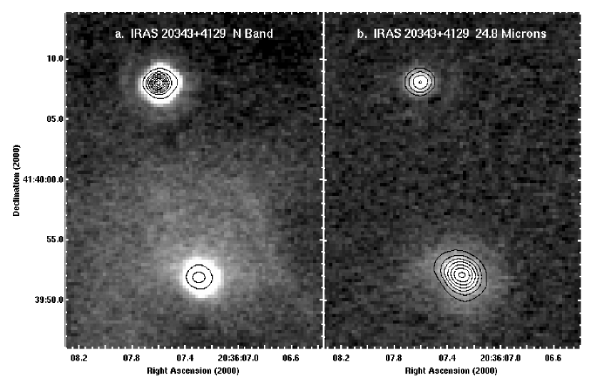
Figure 1: IRAS 20343+4129 in N band centered at 10.5 $\mu$m (a) and at 24.8 $\mu$m (b). IRS 1 is in the NE, and IRS 3 in the SW. The grayscale is adjusted to show extended emission. Eight equally spaced contours indicate the relative peak strength and extension for the central regions of the sources. Flux densities and FWHM are given in Table 1. The true source positions are most likely to be at the K band positions of IRS1: 20^h36^m7.6^s, 41$\arcdeg 40\arcmin 8\farcs 0$ (J2000) IRS3: 20^h36^m7.3^s, 41$\arcdeg 39\arcmin 52\farcs 5$ (J2000)(Kumar et al., 2002), and the coordinates shown have been adjusted to fit them. The 3.6 cm source of Carral et al. (1999) is within an arcsecond of IRS 3.

Images of 18151 and 20343 IRS 1 appear to be unresolved at both wavelengths with indications of the first diffraction ring. 20343 IRS 3 is marginally resolved at both wavelengths with FWHM a few tens of per cent larger than the PSF. In addition, there is extended diffuse emission surrounding the central peak, especially in N band (Fig. 1a). The extended nature of the central peak of IRS 3 is clearer at 24.8 $\mu$m, and can be seen in Fig. 1b. FWHM values of Gaussian fits to the profiles by IRAF are shown in Table 1. Our survey observations and “pipeline” image processing did not emphasize the highest possible S/N for source and PSF profiles intended for image deconvolution. We characterize the PSFs by values shown in Table 1 that are averages of Gaussian FWHM values and their standard deviations from calibration star observations over the course of the night. The standard deviation in the PSF could be due to small errors in shifting individual images before averaging and/or varying seeing in the unstable atmosphere.

2.2 MIRSI Grism Spectra on the IRTF

Grism spectra of the sources were obtained on 2003 September 14. The MIRSI grism was used with an N band prefilter, cutting off the spectra just longward of [Ne II] 12.8 $\mu$m. The slit was oriented NS, and the system can be thought of as a long slit spectrometer. On E. Tollestrup’s suggestion, we arranged both chop and nod to be NS so that four spectra were recorded in each nominal 30 second integration camera frame, giving total on-source time of 120 seconds per camera frame. We experienced considerable difficulty centering the source on the slit, and only one of the chop-nod images could be well centered on the slit at best. For each source, multiple nominal 30 second integration frames were taken, although not all could be used due to the source drifting off the slit or excessive noise.

The initial spectral processing involved the following steps: (1) For each chop-nod subtracted camera frame, the electronic pattern noise was determined from the channel of the chip blanked by the N band filter’s long wavelength cutoff, and subtracted. (2) The frames were flat-field corrected using a dome flat from which a dark frame had been subtracted. (3) All camera frames were averaged into a single combined frame with the IRAF task combine. (4) Copies of the combined frame were inverted and shifted as necessary, and then all four chop-nod spectra were averaged to a single combined spectrum using the combine task. (5) A bad pixel mask was applied to the single combined spectrum. (6) Each channel’s dark sky baseline surrounding the combined spectrum was inspected for an offset. If an offset was found, the median level was shifted to obtain zero baseline outside the spectrum. This processing proved capable of recovering spectra where there was no signal visible in raw data frames. 18151 had strong signal visible, but both sources in 20343 appeared only barely visible after the first stage of pattern noise correction. IRS1 suffered from a noisy portion in its two best frames between 10 and 11 $\mu$m. 22% of the pixels in the spectrum in this wavelength band had excessive noise and were zeroed. The final flux densities were corrected for the zeroed pixels.

For the sources here, $\mu$ Cep, an M supergiant, was used to calibrate the spectra. M supergiants are variable, and less desirable than the K giants used as photometric standards, but $\mu$ Cep gave an extremely high S/N calibration spectrum. The $\mu$ Cep grism spectra were processed in the same way as the candidate HMPO spectra. The IRAF task apall was used to extract the candidate HMPO spectra and the $\mu$ Cep spectrum. A linear grism dispersion relation was created using the telluric lines near 10 $\mu$m and the [Ne II] 12.8 $\mu$m  line. The atmospheric transmission spectrum was taken from the UKIRT web site, convolved with the grism response, and cross-correlated to the uncalibrated MIRSI $\mu$ Cep spectrum to determine one wavelength-pixel point. The [Ne II] 12.8 $\mu$m line was used from the IRAS 18247-1147 spectum in which it was detected for the second point.

In order to use our $\mu$ Cep spectrum for flux calibration, we obtained ISO SWS spectra from the University of Calgary web site. This site uses a program to extract spectra as given by Sloan et al. (2003). Three spectra are available for $\mu$ Cep, and they show some minor differences. We chose TDT 05602852 for $\mu$ Cep because it appeared best based on inspection of separate up and down scans kindly provided by Kraemer (2006). A custom IDL procedure was used to calibrate the candidate HMPO spectra to the ISO $\mu$ Cep flux densities. It multiplied each uncalibrated candidate HMPO spectral point by the ratio of the the ISO calibrated spectral point (convolved to the same resolution as the MIRSI grism) divided by the uncalibrated MIRSI point for $\mu$ Cep. This process gave us a preliminary calibrated spectrum. However, we did not know how well the sources were centered on the slit, so a final step was made, following a suggestion by E. Tollestrup. For each preliminary calibrated spectrum, the flux densities, $F_{\lambda}$, were summed over the spectrum, and the sum compared to the flux, $F$, as measured photometrically through the N band filter. Their ratio was used as a correction factor for preliminary calibrated spectrum. Flux densities in Janskys, $F_{\nu}$, were calculated from $F_{\lambda}$ for presentation in this paper. The calibrated spectra are shown in Figure 2. The 24.8 $\mu$m flux densities in Table 1 compared to the spectra indicate that the SEDs all rise significantly with increasing wavelength.

2.3 TEXES Spectra on the Gemini North

High spectral resolution observations of 20343 IRS 1 and IRS 3 were made during the Texas Echelon Cross Echelle (TEXES) Demonstration Science run on the Gemini North 8-m telescope in July 2006 as part of the program GN-2006A-DS-2. TEXES is a cross-dispersed mid-infrared (5-25 $\mu$m) spectrograph capable of 0$\farcs$4 and 3 km s^-1 resolution on Gemini (Lacy et al., 2002). All data from the Demonstration Science run are publicly available at http://archive.gemini.edu.

The TEXES candidate HMPO observations were made in the TEXES hi-med spectroscopic mode with a 0$\farcs$5 slit giving $\sim$ 4 km s^-1 resolution. The slit length was $\sim 4\arcsec$, oriented EW, with 0$\farcs$15/pixel sampling along the slit. Two observing modes were used: nod mode, in which the telescope was nodded at $\sim$ 0.1 Hz to move the source by $1\farcs 7$ along the TEXES entrance slit, and scan mode, in which the telescope was moved south across the sky in 0$\farcs$25 steps without nodding to map the object.

Two spectral regions were observed, centered at [Ne II] (12.8 $\mu$m) and at [S IV] (10.5 $\mu$m). The spectral coverage at each setting was $\sim$ 0.6%. Spectral calibration was determined from sky emission lines, and is accurate to 1 km s^-1. Intensity calibration was obtained from observations of an ambient temperature blackbody, and for scan mode observations is accurate to $\sim$ 20%. In nod mode, there is an additional uncertainty due to the unknown fraction of the flux outside of the 0$\farcs$5 slit. For compact sources this is a random uncertainty due to seeing and guiding, whereas for extended sources it causes a systematic underestimate of the flux. In addition, for both nodded and mapping observations the sky subtraction procedure introduces an uncertainty due to the possibility of emission in the sky position.

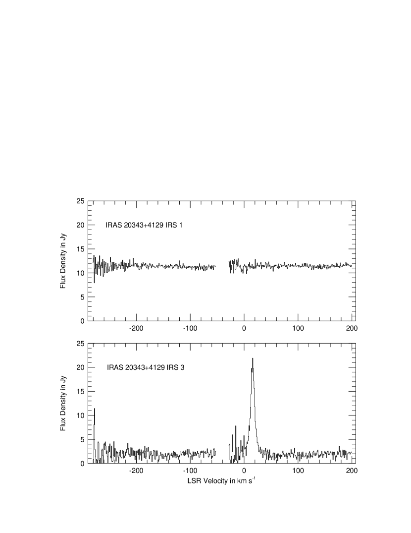
Figure 3: TEXES spectra of IRAS 20343+4129 IRS 1 and IRS 3 for [Ne II] plotted in velocity with respect to the local standard of rest. The [Ne II] line in IRS 3 has its center at $V_{LSR}=15.7\pm 1$ km s^-1 ($\lambda=12.814\ \mu$m or $\nu=780.383$ cm^-1 after correcting for the Earth’s motion relative to the LSR). The gap in each spectrum at $V_{LSR}\sim-40$ km s^-1 is between grating orders.

20343 IRS 1 was observed only in the nod mode at the [Ne II] setting. Its 12.8 $\mu$m continuum was clearly detected, with 11.5 Jy measured through the 0$\farcs$5 slit. This flux is in agreement with the MIRSI grism spectrum. No scan map was made, but the source’s extent along the slit was less than 0$\farcs$5. There was no evidence of the [Ne II] line in the spectrum, which is shown in Figure 3. The equivalent width for a narrow ($<$ 10 km s^-1) line was less than $2.0\times 10^{-3}$ cm^-1, indicating that the line flux from a 0$\farcs$5 region was less than $6\times 10^{-18}$ W m^-2 (2$\sigma$ uncertainties). We note that the line flux could be greater than our limit if the line source is more extended than the continuum source or if the line is broad. A 100 km s^-1 wide line would have to be $2\times 10^{-17}$ W m^-2 to be detected. In addition, the line would have been missed entirely if it were at V_LSR = -20 to -50 km s^-1, which fell between TEXES grating orders, but this would require a velocity shift of $>$30 km s^-1 from the molecular cloud velocity of +11 km s^-1.

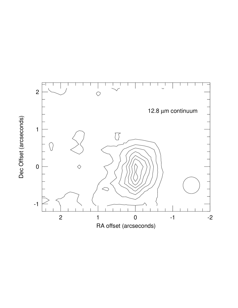
Figure 4: TEXES scan-mode 12.8 $\mu$m continuum map of IRAS 20343+4129 IRS 3. The contours are at $1.67,3.34,...11.7\times 10^{10}$Jy sr^-1 The beamsize of $0\farcs 5$ is shown in the lower right.

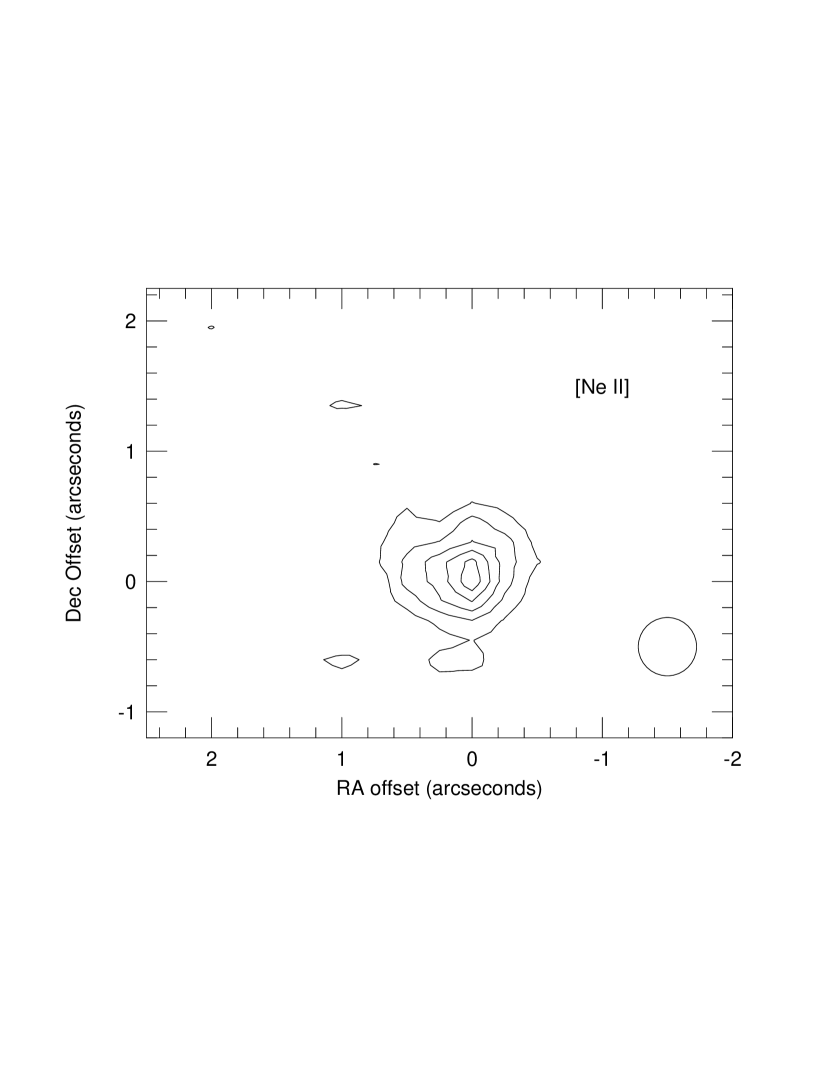
Figure 5: TEXES scan-mode [Ne II] (12.8 $\mu$m) line map of IRAS 20343+4129 IRS 3. The contours are at $2.0,4.0,...10.0\times 10^{-6}$ W m^-2 sr^-1. The beamsize of $0\farcs 5$ is shown in the lower right.

20343 IRS 3 was observed at the [Ne II] setting in both nod mode and scan mode. The nod mode observations have higher signal to noise ratio, but have increased flux calibration uncertainty. The nod mode spectrum and the scan-mode continuum and line maps are shown in Figures 3, 4, and 5. The 12.8 $\mu$m continuum flux, derived from a sum over a $1\farcs 35\times 1\farcs 25$ region where flux is apparent in the map, is 2.3 Jy. This is about 40% of the flux in the MIRSI grism spectrum, suggesting that some extended emission was missed. For the nod mode observations, the nod throw was $1\farcs 7$ EW, and for the scans the sky background were taken from positions $1\farcs 5$ north and south of the peak. Consequently, emission on a scale $>1\farcs 5$ would have been missed. The continuum source appears extended NS in the TEXES map, and possibly double-peaked. Its extent is roughly consistent with the size of the MIRSI 10.5 $\mu$m N band image (Table 1; §3.1). The more extended 24.8 $\mu$m emission is elongated along a NW-SE axis rather than NS (Figure 1; Table 1; §3.1). [Ne II] was clearly detected with a spectrally resolved line-to-continuum ratio of $\sim$ 10. The [Ne II] distribution appeared more point-like than the continuum distribution, and is located on the northern end of the extended continuum source (see Figures 4 and 5). The line is centered at $V_{LSR}=15.7\pm 1$ km s^-1 with an observed FWHM $\sim$ 8 km s^-1. The line flux from the map is $1.0\times 10^{-16}$ W m^-2.

We attempted to observe IRS 3 in the [S IV] setting, but failed to detect either continuum or line emission. The MIRSI grism spectrum indicates that the 10.5 $\mu$m continuum is a factor of about 2 weaker than the 12.8 $\mu$m continuum, so it should have been detected, although not easily since the TEXES sensitivity is a factor of about 2 poorer at 10.5 $\mu$m. Given the possiblity of a pointing error, especially since this was the first science run for TEXES on Gemini, we choose not to quote an upper limit from these observations.

3 Models of the Mid-IR Emission

3.1 Overview of a Simple Dust Continuum Model

The geometry of the mid-ir emitting dusty clouds is unknown except for constraints on their projected diameters. We can make simple three-component models to match our spectra and photometric data, and the models will give estimates of the temperatures of the dust clumps, the column densities through them, the clump masses, and the mid-ir luminosities. Our models should not match the SEDs outside the mid-ir: we would expect them to underestimate the observed SED at both ends of the spectrum.

The model components are (1) a hot component whose size is constrained by the N band image, (2) a warm component whose size is constrained by the 24.8 $\mu$m image, and (3) a cold, pure extinction component that is responsible for the silicate feature. In order to understand clearly the relationships of the various model inputs, we review the emission of an isothermal, constant density, dusty clump observed through a colder cloud that creates extinction but no emission. The observed flux density, $F_{\lambda}$, is given by

$$F_{\lambda}=\Omega B_{\lambda}(T)(1-e^{-{\tau_{e}(\lambda)}})e^{-\tau_{a}(\lambda)}$$ (1)

where $\Omega$ is the solid angle of the clump, $B_{\lambda}(T)$ is the blackbody intensity, $\tau_{e}(\lambda)$ is the optical depth of the emitting clump, and $\tau_{a}(\lambda)$ is the extinction optical depth of the absorbing (and scattering) overlying cloud. In general, emissivity, $\epsilon(\lambda)=(1-e^{-\tau_{e}(\lambda)})$, but for an optically thin clump $\epsilon(\lambda)=\tau_{e}(\lambda)$. The optical depth in emission is given by

$$\tau_{e}(\lambda)=K_{e}(\lambda)\int\limits_{Clump}\rho_{d}dl$$ (2)

where $K_{e}(\lambda)$ is the absorption cross section per mass of the emitting dust in cm² g^-1, $\rho_{d}$ is the mass density of the dust, and the integral is through the emitting clump. The integral through the clump can be related to the column density of H nucleons, $N_{H}$ through

$$\int\limits_{Clump}\rho_{d}dl={{M_{d}}\over{M_{g}}}\mu m_{H}N_{H}$$ (3)

where ${M_{d}}\over{M_{g}}$ is the dust to gas mass ratio, $\mu$ is the mean molecular weight for the assumed abundance ratios, assuming neutral atomic gas instead of H₂ in order to follow the convention of Draine (2003a) that uses the column density of H nucleons, and $m_{H}$ is the mass of a hydrogen atom. Thus the emission optical depth can be related to the column density:

$$\tau_{e}(\lambda)=K_{e}(\lambda){M_{d}\over M_{g}}\mu m_{H}N_{H}$$ (4)

We can now clearly see from equation (1) that the observed flux density, $F_{\lambda}$ is related to both the solid angle and the column density, and that the derived column density is strongly dependent on the assumed solid angle. For the simple geometry of a constant density, end-on cylindrical cloud whose solid angle is estimated from the observed angle, $\theta_{FWHM}$, $\Omega={\pi\over 4}\theta_{FWHM}^{2}$, and in the optically thin case

$$F_{\lambda}={\pi\over 4}\theta_{FWHM}^{2}B_{\lambda}(T)K_{e}(\lambda){M_{d}\over M_{g}}\mu m_{H}N_{H}e^{-\tau_{a}(\lambda)}$$ (5)

The assumed projected diameter of the clump is thus clearly a key factor in deriving a reasonable column density. For optically thick clouds, the exponential function in the expression for emissivity makes the column density estimate very strongly dependent on the assumed diameter.

A simple approximate way of estimating source diameters from the IRTF images for marginally resolved sources like 20343 IRS 3 (see Table 1) is based on assuming that the profiles of the true source, the observed data, and the PSF are all Gaussians. With this assumption (that is certainly not correct for an Airy disk), a formal deconvolution would give

$$\theta_{s}=\sqrt{\theta_{d}^{2}-\theta_{p}^{2}}$$ (6)

where $\theta_{s}$ is the true source FWHM, $\theta_{d}$ is the observed data FWHM, and $\theta_{p}$ is the PSF FWHM. The resultant $\theta_{s}$ are $0\farcs 75$ and $1\farcs 57$ in the N and 24.8 $\mu$m filters, respectively. In this case however, the source extent at the shorter wavelength is more accurately determined by TEXES at 12.8 $\mu$m on Gemini. Calculated in the same way, the extent is $0\farcs 56\times 1\farcs 1$ EW $\times$ NS, with area equivalent to a circular source of $0\farcs 80$.

For the unresolved sources 18151 and 20343 IRS 1 we can make estimates of the source sizes from the IRTF observations based on Gaussian deconvolutions as follows. Let us represent $\theta_{d}$ in terms of $\theta_{p}$ and $n$ standard deviations of the PSF FWHM, $\sigma_{p}$: $\theta_{d}=\theta_{p}+n\sigma_{p}$. Substituting this expression into Eq(6) gives

$$\theta_{s}=\sqrt{2n\sigma_{p}\theta_{p}+n^{2}\sigma_{p}^{2}}$$ (7)

An observation of a source with a true value of $\theta_{s}$ in which the statistical variation resulted in a $-n\sigma_{p}$ deviation from $\theta_{d}=\theta_{p}+n\sigma_{p}$ would appear to be unresolved with observed $\theta_{d}=\theta_{p}$. Thus we can estimate reasonably likely values for source size $\theta_{s}$ from a $1\sigma$ deviation by substituting $n=1$ into Eq (7), and a $3\sigma$ upper limit to a source size by substituting $n=3$. The resulting values of $\theta_{s}$ are larger than $\sigma_{p}$ or $3\sigma_{p}$ because of the deconvolution. Table 2 presents diameters for the hot components and the warm components calculated from the Gaussian FWHM values in Table 1 in N band and at 24.8 $\mu$m, respectively. They have been converted to AU at the distances of the HMPO candidates for the table. The diameters in Table 1 are consistent with those of disk candidates associated with HMPOs cited by Cesaroni et al. (2007), most of which have diameters from 1000-3000 AU.

The derived column densities depend on the dust model that specifies $K(\lambda)$. A very attractive model is that of Ossenkopf & Henning (1994) for protostellar cores often referred to as OH5. This dust represents coagulated grains with ice mantles that would be expected to form from dust originally in the diffuse interstellar medium during the process of molecular cloud formation. It has been used to fit submm SEDs of high-mass protostellar cores (van der Tak et al., 1999, 2000) and far-ir observations of the UC HII region G34.3+0.2 (Campbell et al., 2004). However, when we examined its $K(\lambda)$ behavior around 10 $\mu$m, we found that its silicate feature is shifted longward from 9.7 $\mu$m and broadened so that it does not appear to be compatible with our grism spectra. Models by Draine (2003a, b) and colleagues fit the shape of our observed silicate absorption feature well. We have chosen their 2003 $R_{V}=5.5$ synthetic extinction curve (Draine, 2003a) for dust in dense clouds in the Milky Way. It is accessible on the web and well documented. We have also fit the data successfully with $R_{V}=3.1$ dust for diffuse clouds, but $R_{V}=5.5$ dust is appropriate for dense clouds and the deduced column densities should be more realistic. The dust model has ${M_{d}\over M_{g}}=105$. Roman-Zunga et al. (2007) recently found the $R_{V}=5.5$ dust to fit 1.2 - 8.0 $\mu$m data from the dense core Barnard 59. In retrospect, we found high enough temperatures that ice mantles should have evaporated so that the OH5 dust would not be expected to fit our data.

Fitting the shape of the grism spectrum of 18151 (Figure 2) and the large flux density at 24.8 $\mu$m (Table 1) requires a minimum of three components for our models: hot dust responsible for the 8 $\mu$m end of the grism spectrum, warm dust for the 13 $\mu$m end of the spectrum and the 24.8 $\mu$m photometry, and cold dust for the depth of the silicate absorption. The model calculation has the following input parameters: the temperature of the hot component, $T_{h}$, the diameter of the hot component $\theta_{h}$, the optical depth in emission of the hot component at 9.70 $\mu$m, $\tau_{h}$, the analogous parameters for the warm component, $T_{w}$, $\theta_{w}$, and $\tau_{w}$, and the extinction optical depth, $\tau_{a}$, of the overlying cloud that is too cold to emit in the mid-ir. In the mid-ir, the extinction is virtually pure absorption. The model uses a spectrum that is the sum of the contributions of both hot and warm components each calculated according to Eq(1) to fit the observations. For given optical depths, column densities, $N_{H}$, can be derived from Eq(4) for each component, using parameters found in Draine’s web site for the dust model. For end-on cylindrical geometry, the masses of the hot and warm components can be derived from $N_{H}$ for each. Visual extinctions are calculated from the extinction cross section per H nucleon at the center of the V band as given in the web site and $N_{H}$ for the cold absorbing component. The SED due to the two dust clumps and overlying extinction is calculated to verify that it does not create excessive emission outside the mid-ir, and to derive the luminosity of the mid-ir emitting clumps for comparison to measurements and estimates of the overall candidate HMPO luminosity.

3.2 Fitting the Continuum Data

Our goal is to apply our simple three-component model to the grism and 24.8 $\mu$m photometric data to derive estimates of the temperatures, the column densities, the masses, and the luminosities of the emitting dust components, and the column density of the cold extinction component. We have no measurements of the angular extents of the components for 18151 or 20343 IRS 1 because they were unresolved, although we do have them for 20343 IRS 3. If we assume incorrectly small sizes for the first two, we will make over-estimates of the column densities. We have chosen to use large size estimates that are consistent with the data for these two so that our column densities can be thought of as lower limits to the true values. The parameters for our models are shown in Table 3. Table 3 shows sizes based on 1 $\sigma$ deviation estimates for unresolved sources in Table 2. For 20343 IRS 3, it uses the size from the TEXES continuum map for the hot component, and the size based on Gaussian deconvolution of the MIRSI 24.8 $\mu$m image for the warm component.

The models were interactively fit to the data. In order to quantify the quality of the fit and to aid in choice of extreme values of the parameters consistent with the systematic accuracy of the data, we defined a modified $\chi^{2}$ statistic. The grism spectra were broken into four photometric bands: $8.0-9.0\mu$m, $9.0-10.5\mu$m, $10.5-12.0\mu$m, and $12.0-13.0\mu$m. Fluxes were summed in each band. The 24.8 $\mu$m photometry served as a fifth band. We defined the modified $\chi^{2}$ statistic for each band, $i$, as

$$\chi^{2}_{mi}=\frac{{(F_{i,Model}-F_{i,Data})}^{2}}{{F_{i,Data}}^{2}}$$ (8)

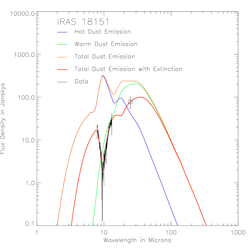
Figure 6: Model individual and summed hot and warm components SEDs before extinction, and with extinction for IRAS 18151-1208 compared to the MIRSI-IRTF data. This model has a hot component temperature $T_{h}=455$ K. Other parameters of the model are given in Table 3. Emission from the hot and warm components before extinction are shown in blue and green, respectively, and their sum, the total dust emission inside the outer cold cloud, is shown in orange. The model’s observed emission after extinction by the overlying cold cloud is shown in red, and the data are shown in black.

where $F_{i}$ is the flux in band $i$. The sum of the five terms formed $\chi^{2}_{m}$ for the model. This statistic places the quality of the fit as a fraction of the data value in each band on equal footing. Even though it assumes that each of the five bands has equal S/N and has no specific statistical interpretation, it is useful for fitting models to the data. For optimizing models, we sought to minimize $\chi^{2}_{m}$ interactively, initially using graphs of the models plotted over the data as guides, rather than using an exhaustive, automated search through the parameter space. Such an automated search is not justified by the quality of the data and the simplicity of the model. Final models in Table 3 were optimized using $\chi^{2}_{m}$ values. For choosing the upper or lower value of a specific parameter (e.g. $T_{w}$) that might be reasonable, we started with the value in an optimum model, and varied that parameter (only) until the band most affected by the parameter (in this case $i=5$, $24.8\mu$m) indicated a 30% difference (our systematic photometric accuracy), or $\chi^{2}_{mi}=0.09$. On a graph of the data like Figure 6, the upper value $T_{w}$ would cause the model’s flux density to fall on the end of the upper error bar at 24.8 $\mu$m. It was not feasible to vary more than one parameter at a time because of the size of the parameter space and the fact that all bands of our data were somewhat affected by all of the parameters. The procedure is arbitrary. Larger extreme values for a parameter of interest could be found if all others were also varied compensating for the changed parameter of interest (e.g. if $T_{h}$ were the parameter of interest, a larger extreme value would result if $\tau_{h},T_{w},\tau_{w},$ and $\tau_{a}$ were varied in addition to $T_{h}$).

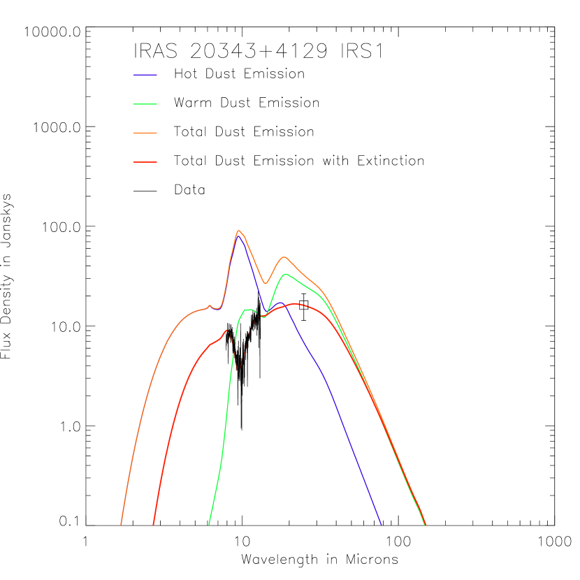
Figure 7: Model individual and summed hot and warm components SEDs before extinction, and with extinction for IRAS 20343+4129 IRS 1 compared to the MIRSI-IRTF data, as in Fig. 6. Parameters of the model are given in Table 3.

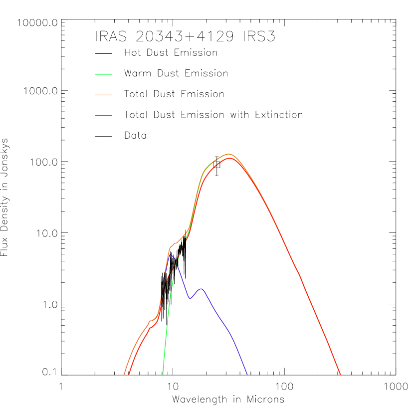
Figure 8: Model individual and summed hot and warm components SEDs before extinction, and with extinction for IRAS 20343+4129 IRS 3 compared to the MIRSI-IRTF data, as in Fig. 6. Parameters of the model are given in Table 3.

The best-fit temperatures of the hot and warm components are in the ranges 420-1000 K and 110-182 K, respectively. It is useful to examine SEDs over a wide range of wavelengths in order to understand how the components combine to fit the data. We show the SEDs of individual components in Figure 6 for the model of 18151 with a 455K hot component whose parameters are given in Table 3. Figures 7 and 8 show models for 20343 IRS 1 and IRS 3, and their model parameters are also shown in Table 3. In addition, Figures 6-8 show the combined SEDs both with and without the cold components’ extinction, and the IRTF data. In Figure 6, the 455K hot component shows a strong 9.7 $\mu$m silicate emission feature, as expected. However the 136K warm component does not show a strong emission feature because its Planck spectrum is rapidly rising to long wavelengths and the silicate feature is smoothed out because it is optically thick in its center. Absorption features at 9.7 and 18 $\mu$m due to the cold layer are clear in the total spectrum, and the latter causes a nearly flat portion between 15 and 20 $\mu$m. This shape in the mid-ir is not necessarily an artifact of the simplicity of a three component model. A similarly shaped SED is shown from the library of Monte Carlo radiative transfer models at http://caravan.astro.wisc.edu/protostars/ for the low mass protostar IRAS 04368+2557 by Robitaille et al. (2007). Our model SED for 18151 in Figure 6 also clearly shows that these components emit very weakly at both near-ir and submm wavelengths. For 18151, a large range in $T_{h}$ will fit the data apparently because the grism spectral range could lie in the Raleigh-Jeans part of the hot component’s spectrum for high values of $T_{h}$. The $T_{h}=455$ K model is in the lower end of the range. A model with $T_{h}=1600$ K, a commonly assumed dust sublimation temperature (Whitney et al., 2004), will fit our data, but would have a large excess over the observed flux at 2.1 $\mu$m (Davis et al., 2004). A model with $T_{h}=1000$ K is presented in Table 3 that fits both our data and the flux at 2.1 $\mu$m.

3.3 General Results and Discussion for the Continuum Models

Parameters for the models are presented in Table 3. Two models are given for 18151 at extreme ends of the range of $T_{h}$ that fit the data well, and the best-fit model is given for each of 20343 IRS 1 and IRS 3. The summed values of $\chi^{2}_{m}$ are given in the last column. In addition, upper and lower extreme values that are consistent with the data to within 30% as discussed above are shown.

There are a number of important aspects of the values derived from the models. The first is that the source that appears most deeply embedded, 18151, could have a hot component with a sufficiently high temperature so that its mid-ir would be on the Raleigh-Jeans end of the spectrum, so that the temperature cannot be determined without measurements in shorter bands like K, L or M. However, it is entirely likely that some or all of the flux at these shorter bands would come from an additional, hotter dust component than the ones whose mid-ir we seek to model. For the other two objects, Table 3 shows moderate ranges in temperatures from lower to upper values that are compatible with the best-fit emission optical depths. The range of temperatures that could be fit by varying the emission optical depths at the same time with only modest increases in $\chi^{2}$ would be larger than shown. Nevertheless, we feel the temperatures shown are realistic estimates. The ranges in $T_{h}$ and $T_{w}$ are well separated in all of the sources. If each source’s emission is from a single clump or disk with a continuous range in temperatures, each must contain a wide range in the actual temperatures.

It is interesting to note that the temperatures for what we call warm dust, $T_{w}$, are rather close to those of the “hot component” of Sridharan et al. (2002) based on IRAS data ($T_{hd}$, of 170 K and 150 K for 18151 and 20343, respectively). It suggests that our IRTF measurements are measuring much of the same dust as the shorter IRAS bands measured. In fact, our N band $F_{\nu}$ values for 18151 and 20343 IRS 1 + IRS 3 are each slightly more than 50% of the IRAS PSC values. Our 24.8 $\mu$m $F_{\nu}$ for 18151 virtually equals the IRAS PSC 25 $\mu$m value, and the sum of the 20343 24.8 $\mu$m $F_{\nu}$ values is 2/3 of the IRAS 25 $\mu$m value.

Another interesting aspect is the extremely small amount of gas and dust in the hot components. This hot material is unlikely to be a major part of accretion disks that might be expected for HMPOs, because the accretion disks are likely to contain about the same mass or more as the stars, and to have characteristic temperatures from ten to several hundred K (Cesaroni et al., 2007). It could be in a hot inner rim or surface layer of a photoevaporating disk (Hollenbach et al., 1994). The assumed diameters of the mid-ir components suggest that the emission comes from material that might be described as being in an outflow cavity wall. In fact, it may be coming from the intersection of a flared accretion disk with the surface of the outflow cavity, as has been suggested for other sources by De Buizer (2007b). Although the assumed diameters of the hot components are somewhat arbitrary and affect $N_{H,h}$, they do not affect the mass estimates since these components are optically thin. The ranges about the central value of $N_{H,h}$ and $M_{h}$ are about $\pm 30\%$, as expected for optically thin sources. (Lower limits to $N_{H,h}$ based on the 3$\sigma$ upper limits on source diameters shown in Table 2 can be calculated from the data in Table 3 since $N_{H}$ is inversely proportional to $\Omega$ for optically thin sources.) Accurate estimates of $N_{H,h}$ and number density $n_{H,h}$ of the hot components of 18151 and 20343 IRS 1 will require higher resolution observations on a larger telescope.

The optical depths in emission of the warm components, $\tau_{w}$, are high in the cases of 18151 and 20343 IRS 3, 4.2 and 0.9, respectively. This effect is a surprise because the assumed values of the projected diameters $D_{w}$ are not particularly small compared to observed and expected diameters for structures like candidate accretion disks near HMPOs, (De Buizer & Minier, 2005; Shepherd et al., 2001; Cesaroni et al., 2007). While 18151 was unresolved and its value for $N_{H,w}$ is essentially a lower limit, IRS 3 was resolved, so its value for $N_{H,w}$ is a firmer estimate. For these two HMPO candidates, indicated $N_{H,w}$ values are about as large as the column density for extinction, $N_{H,a}$. Even with these high values, however, the masses are less than 1 M_☉ and much less than the mass expected for an HMPO. This situation again indicates that the mid-ir emitting dust is not tracing the bulk of the mass expected to be in accretion disks.

Our mass estimates have led to the conclusion that in these three HMPO candidates, mid-ir emission is not indicating massive accretion disks. Either only a small fraction of their mass is emitting in the mid-ir, or the disks have been disrupted already. The emission may well come from dust in and around the walls of outflow cavities as has been suggested for other HMPOs by De Buizer & Minier (2005) and De Buizer (2006, 2007a) and as is indicated in the two dimensional radiative transfer models for a low mass class I protostar of Whitney et al. (2003a).

Extinction optical depths, $\tau_{a}$, are not extremely high, and cover a limited range. There is a selection effect: if they were larger, the HMPO candidates would not have been included in the original survey for lack of 12 $\mu$m IRAS detection, or we might not have detected the HMPO candidates in the mid-ir on the IRTF. (Five of 23 fields chosen from the Sridharan et al. (2002) survey resulted in non-detections in N band on the IRTF.) The appearance of the 20343 IRS 3 grism spectrum suggested that there might not be any extinction, but fitting the spectrum required all of the components. In some cases, the range in $\tau_{a}$ from lower to upper value is small because the extinction is exponential and the sources are optically thick in extinction. The values of $N_{H,a}$ and $A_{V}$ are also not extreme since they are directly proportional to $\tau_{a}$. Unlike the emitting components, the extinction $\tau_{a}$ and parameters derived from it ($N_{H,a}$ and $A_{V,a}$) are not affected by the assumed source size, and hence are more firmly defined values.

High mass stars are expected to form at the centers of cluster-forming molecular cloud cores (Beuther et al., 2006). In our small sample of three objects, only 18151 appears to be centered on a 1.2 mm continuum core in the plane of the sky. Comparison of the column density of H nucleons per cm², $N_{H,a}$, and the visual extinction in magnitudes, $A_{V,a}$, from the mid-ir model to the values for column density of H₂, $N_{gas}$, and $A_{V}$ from 1.2 mm observations given by Beuther et al. (2002a) would indicate if the candidate HMPO is indeed centered along the line of sight within the larger 1.2 mm dust core if a consistent dust model and units were used at both wavelengths. If the HMPO candidate were at the core center, interior to the bulk of the 1.2 mm dust core’s mass, we would expect the mid-ir based column density for the cold component to be due to near side of the dust core, and have one-half the column density based on the 1.2 mm observation. For a consistent comparison, we have calculated $N_{H}$ from equation (5) using Draine (2003a) dust, the peak flux of 673 mJy for $(11\arcsec)^{2}$ at 1.2 mm given by Beuther et al. (2002a) in their Table 2, $T_{dust}=T_{cd}=47$K given by Sridharan et al. (2002) in their Table 1, and the solid angle of $(11\arcsec)^{2}$ in place of ${\pi\over 4}\theta^{2}_{FWHM}$. The Draine (2003a) $R_{V}=5.5$ dust model has $K_{e}(1.2\rm{mm})=0.2388$ cm²  g^-1 and $A_{V}=7.29\times 10^{-22}N_{H}$, where $N_{H}$ is the column density of H nucleons. For 18151, the 1.2 mm results are $N_{H}=5.6\times 10^{23}\ \rm cm^{-2}$ (log$N_{H}=23.75$) and $A_{V}=410$. One half of the column density would give log$N_{H}=23.45$ and $A_{V}=205$. These values are a factor of 2.8 larger than the mid-ir based values in Table 3, log$N_{H,a}=23.00$, and $A_{V,a}=72.1$. It appears that the mid-ir source is not at the center of the 1.2 mm emitting core, but near its front side. However, there are significant uncertainties in the estimates. We have ignored the column densities of hot and warm dust in emission in the mid-infrared, but their size $\sim 1\arcsec$ on the sky should not have contributed significantly to the 1.2 mm emission detected in an 11$\arcsec$ beam. The largest uncertainty lies in the value of $K_{e}(1.2\rm{mm})=0.2388\ cm^{2}\ g^{-1}$. For far-ir through mm wavelengths, the emission coefficient is often approximated as $K\propto\lambda^{-\beta}$. Draine (2003a) $R_{V}=5.5$ dust has $\beta=1.8$ between 250 $\mu$m and 1.2 mm. Based on a sample of 69 HMPO candidates, Williams et al. (2004) derive a mean $\beta$ of 0.9, that would increase $K_{e}(1.2\rm{mm})$ by 4.1, and decrease the column density to give log$N_{H}=22.84$ and $A_{V,a}=50.1$, in much better agreement with the mid-ir based results. In fact, one could turn the problem around. For cases where there is strong evidence that an HMPO is centered in a core, the ratio of column densities determined by the extinction at 9.7 $\mu$m and 1.2 mm dust emission determines the overall slope of the extinction curve between them, if one assumes a wavelength in the far-ir at which $K_{e}(\lambda)$ flattens. Using 250 $\mu$m as the reference wavelength (e.g. Hildebrand (1983)), the mid-ir derived column density $N_{H}=1.0\times 10^{23}$ cm^-2, and 1/2 of the 1.2 mm flux density to account only for the emission in front of the HMPO, we find $\beta=1.2$.

There are other possible reasons for discrepancies. For cores that do not fill the 1.2 mm radio beam, one would expect the difference in telescope beams to affect the ratio of column densities, with the larger beam 1.2 mm $N_{H}$ being less than the smaller infrared beam $N_{H}$. Conversely, an unresolved clumpy structure in the 1.2 mm emitting core could result in higher 1.2 mm beam-averaged value than observed in a small diameter infrared beam that happens to pass between clumps giving a low extinction line of sight to the HMPO. Similarly, viewing the source along an outflow cavity as modeled by Whitney et al. (2003a, b, 2004) would result in lower ir-based $N_{H}$ and $A_{V}$. However, the outflows observed for these objects appear to lie in or near the plane of the sky (see §4).

The HMPO candidates 20343 IRS 1 and IRS 3 are not projected against peaks in the 1.2 mm emission (Palau et al., 2007). Nevertheless we can estimate $N_{H}$ and $A_{V}$ for them from the 1.2 mm map (Beuther et al., 2002a; Palau et al., 2007) that shows $\sim 200$ mJy/($11\arcsec)^{2}$ for both. The ratios of mm-based $N_{H}/2$ to ir-based $N_{H}$ are 1.5 and 5.9 for IRS 1 and 3, respectively, in comparison to 2.8 for 18151. These are consistent with IRS 1 being deeply embedded but not the apparently more evolved IRS 3.

Observations that cover both mid- and far-ir wavelengths are commonly used to estimate the total luminosity of an embedded source (e.g. Sridharan et al. (2002)). For a case in which an HMPO is completely embedded so that the observed infrared emission comes from a circumstellar dust envelope that absorbs and reradiates all of the HMPO’s emission, the total luminosty is accurately measured by the integrated SED. Far-ir observations like IRAS data cover the peak of the SED, but the large beams can include sources in addition to that of the HMPO of interest, especially since high mass stars usually form in clusters. The higher resolution mid-ir observations can be limited to a single HMPO, but lack the far-ir contribution needed for total luminosity. Consequently, luminosity based solely on mid-ir fluxes is usually quoted as a lower limit to total luminosity. Our simple models can be used for lower limit luminosity estimates that account for extinction in the mid-ir and include some flux outside the mid-ir. In Table 3, we show the integrated model SED fluxes that would be observed through the extinction (the red curves in Figures 6-9) as $L_{o}\over L_{\sun}$. We take these model based values as lower limits to the HMPO candidates’ luminosities that are somewhat improved over simply adding our observed mid-ir flux densties.

In Table 3, we also show the summed modeled luminosity emitted by the hot and warm clouds together without the extinction factor applied (the orange curves) as $L_{e}\over L_{\sun}$. If the hot and warm dust components had absorbed all of an HMPO’s power and emitted (re-radiated) it as modeled, the sum of their SEDs would give the total luminosity. Presumably, the cold extinction layer re-radiates in the far-ir the energy it absorbed from the hot and warm components, so an observed full SED extending into the far-ir would have the same luminosity as $L_{e}\over L_{\sun}$. An outflow cavity should not have much effect on the the luminosity estimate. The mid-ir portion of a source’s SED is affected by the line of sight to the cavity, but the far-ir portion that dominates the luminosity is not as strongly affected (Whitney et al., 2003b). Outflow cavities for our sources would have little effect because they appear to be close to the plane of the sky (see §4). Our $L_{e}\over L_{\sun}$ value should be close to the luminosity based on IRAS presented by Sridharan et al. (2002), if we have observed the dominant HMPO and there is little luminosity from the other YSOs. For 18151, our estimate is 22400 $L_{\sun}$ in close agreement with the IRAS-based value of 20000 $L_{\sun}$ (Sridharan et al., 2002). The HMPO candidates 20343 IRS 1 and IRS 3 lie in a single IRAS beam. For 20343 IRS1 and IRS3 combined, our value of $L_{e}\over L_{\sun}$ is 2200 $L_{\sun}$, about two-thirds of 3160 $L_{\sun}$ from IRAS. The star in 20343 IRS 3 is apparently more evolved than the HMPO candidate in 18151 (see §4). As a consequence, it has a lower column density envelope ($N_{a}$) than 18151, so its envelope does not absorb the full stellar emission.

Overall, the $L_{e}\over L_{\sun}$ luminosity estimates agree well with IRAS. Earlier we noted remarkably close agreement between our flux densites and those of the IRAS PSC, and between our $T_{w}$ and the IRAS-based $T_{hd}$ of Sridharan et al. (2002). Consequently the agreement of luminosities is not surprising.

3.4 Analysis of High Resolution Spectra

The infrared fine-structure lines are collisionally excited forbidden lines. As such, they have emissivities proportional to the product of the density of the emitting ion, the electron density, and the collisional excitation cross section, $N_{i}N_{e}q_{lu}$, for $N_{e}<<N_{c}$ (Osterbrock & Ferland, 2006). $N_{c}$, the electron density at which the collisional deexcitation rate equals the radiative deexcitation rate, is $5\times 10^{5}$ cm^-3 for [Ne II] and $2\times 10^{4}$ cm^-3 for [S IV]. The collisional excitation rates are proportional to $T^{-1/2}e^{-E_{u}/kT}$, or about $T^{-0.4}$ for these lines. Since the radio free-free emissivity is proportional to $N_{e}N_{p}T^{-0.35}$, the ratio of the fine-structure line fluxes to the free-free continuum flux is proportional to the ionic abundance relative to that of ionized hydrogen, with a weak dependence on electron temperature and density. The ionic abundances relative to the total atomic abundances depend most strongly on the spectral type, or effective temperature, of the ionizing star, with weaker dependences on the stellar luminosity and the electron density. Consequently, the ratio of the fine-structure line fluxes to the free-free flux and to each other can be used to determine the stellar spectral type.

The most convenient way to determine the stellar parameters that are consistent with the measured fluxes is with a nebular modeling program, such as cloudy (Ferland et al., 1998). We used cloudy (version 07.02.00) to calculate several dust-free models with stellar parameters similar to those of a B2 star, $T_{eff}\sim$ 20,000 K and $N_{Lyc}\sim 4\times 10^{44}$ photons s^-1. An acceptable fit to the observed free-free and [Ne II] fluxes from 20343 IRS 3 was found for $T_{eff}$ = 19,000 - 22,000 K and $N_{Lyc}=3-5\times 10^{44}$ photons s^-1, assuming $N_{e}<<5\times 10^{5}$ cm^-3. The [S IV] flux was predicted to be much less than that of [Ne II], consistent with our failure to detect [S IV].

The extinction-corrected luminosity of IRS 1 is 1380 L_☉ and neither radio free-free nor [Ne II] emission was detected from it, with limits of about 1/3 and 1/15 of the free-free and [Ne II] fluxes from IRS 3. The luminosity and lack of observable ionized gas are consistent with a spectral type of B3 or later, or $T_{eff}<$ 18,000 K, as the ionizing flux of a B3 star is only about 1/10 that of a B2 star (Panagia, 1973).

4 Discussion of Individual Sources

4.1 IRAS 18151-1208

This HMPO candidate was chosen for study because of its deep silicate absorption in the mid-ir (Figure 2), the location of its mid-ir peak at a 1.2 mm peak in the Beuther et al. (2002a) survey, its low level of 3.6 cm emission (Sridharan et al., 2002; Carral et al., 1999), its large-scale CO outflow (Beuther et al., 2002b), its detection in the K band, and the presence of H₂ molecular jets (Davis et al., 2004). At mm and sub-mm, there is a relatively simple peak 13$\farcs 2$ east and $4\farcs 9$ south of the IRAS position with some extension to the southwest (Beuther et al., 2002a; Williams et al., 2004). There is a strong second 1.2 mm peak about $100\arcsec$ west and 33$\arcsec$ south form the IRAS position, and there are two weaker peaks $>80\arcsec$ from it (Beuther et al., 2002a). The main sub-mm peak is within $\sim 2\arcsec$ from the MSX source that we identify with our mid-ir source (Williams et al., 2004). The IRAS and mid-ir luminosity estimates agree well at $\sim 20000$ L_☉ (§3.3), close to that of a B0 ZAMS star (Panagia, 1973). Davis et al. (2004) characterize the K band emission as showing a dense cluster. They conclude that IRS 1, the source at the K band peak, is a pre-UC HII HMPO. It is the only deeply embedded near-ir object in the field (Davis et al., 2004), and it is coincident with the mm peak and with an 0.5 mJy 3.6 cm source (Carral et al., 1999).

For an optically thin HII region, the 3.6 cm flux density of 0.5 mJy would require log $N_{L}$=44.67 ionizing photons s^-1 at 3 kpc, using the common relationship between flux density and number of ionizing photons as given by De Buizer et al. (2005a). This number is that of a B2 ZAMS star (Panagia, 1973), that would have $L=2900$ L_☉ compared to the ir-based luminosity of $\sim 20000$ L_☉. The order of magnitude difference in luminosity could be explained by a significant contribution from lower luminosity members of the cluster, but this seems unlikely since the 24.8 $\mu$m diameter has a 3$\sigma$ upper limit of 3670 AU (Table 2). Apparently, an HMPO at IRS 1 at the pre-UC HII stage is creating the ionization as a hypercompact HII region (HC HII) or as a jet. (In either case the equation used for $N_{L}$ does not apply.) In fact, Davis et al. (2004) found two lines of clumps of shocked H₂ indicating the presence of two jets, one of them centered on IRS 1, and detected Br$\gamma$ at IRS 1. Assuming $A_{V}=30$, they estimated an accretion luminosity of $\sim 120$ L_☉ and inferred a total $L\sim 1000$ L_☉ by extending results from low luminosity YSOs. They argued that these are lower luminosity limits because their $A_{V}$ was calculated for the extended H₂ flow rather than for the source center where we have found $A_{V}=72$. Our value suggests increasing the extinction correction for Br_γ by 83 using Draine (2003a) dust, resulting in an inferred luminosity well in excess of 20000 L_☉.

The large scale CO outflow red and blue shifted lobes are complex (Beuther et al., 2002b). The two jets of H₂ clumps are nearly at right angles, and Davis et al. (2004) interpret the complex CO outflow as consistent with them. Both of the H₂ jets are close to the plane of the sky (Davis et al., 2004), so it is unlikely that our line of sight is along a low extinction outflow cavity. The overall CO outflow distribution and the more powerful H₂ jet both have their centers near IRS 1, while the second jet’s center appears to be about 10$\arcsec$ SW of IRS 1, well outside the mid-ir emission. Davis et al. (2004) estimate the luminosity of the jet centered on IRS 1 to be 0.7 L_☉, and the second jet to have only $\sim 0.05$ L_☉. The H₂ jet luminosity of 0.7 L_☉ is much higher than those in low mass YSOs (Davis et al., 2004). A larger extinction correction for the H₂ luminosity, as suggested above, will increase it significantly. A large outflow luminosity would suggest that it is still strongly accreting.

This source has a Class II CH₃OH maser at its mm peak, but neither an H₂O maser, (Beuther et al., 2002c), nor an OH maser (Edris et al., 2007). (An H₂O maser is associated with the second 1.2 mm source in the 18151 field.) Beuther et al. (2002c) summarize the conditions for models of radiative pumping of the CH₃OH masers as $T\sim 150$ K, methanol column density $N_{M}>2\times 10^{15}$ cm^-2, and $n_{H}<10^{8}$ cm^-3. These are are quite close to the parameters of the warm dust in our mid-ir emission model that has $T_{w}=136$K, and $N_{H}=8.5\times 10^{22}$ cm^-2 with a diameter of 2050 AU. If the source has a line of sight dimension equal to its diameter, the density is $n_{H}=2.9\times 10^{6}$ cm^-3. A recent set of models for CH₃OH maser cites fractional methanol abundance $X_{M}=10^{-5.7}$ (Cragg et al., 2002) that would give methanol column density $N_{M}=1.7\times 10^{17}$ cm^-2. Cragg et al. (2002) cite $N_{M}/\Delta V$ where $\Delta V$ is the linewidth as a key parameter. They give $\Delta V=1$ km s^-1 as typical. With it, our model warm dust component would have $N_{M}/\Delta V=10^{12.23}$ cm^-3 s. Its conditions appear to be comfortably within the conditions for strong 6.7 GHz emission (Cragg et al. (2002) Figure 1). Thus our mid-ir based model density and temperature are consistent with the observed methanol maser emission, and with a pre-UC HII stage for 18151.

For OH masers, the use of $X_{OH}=10^{-6}$ (Cragg et al., 2002) gives $N_{OH}/\Delta V=10^{12.2}$cm^-3 s. This value and $n_{H}=2.9\times 10^{6}$ cm^-3 are in a region of parameter space where OH masers are unlikely for $T_{k}=150$ K (Cragg et al. (2002) Figure 1), consistent with observations.

There have been tentative suggestions that masers might appear in an overlapping sequence of CH₃OH, H₂O, and OH in HMPOs (Beuther et al., 2002c; Cragg et al., 2002), but the evidence does not seem conclusive (De Buizer et al., 2005a). If the sequence were correct it would suggest that 18151 is an early stage HMPO. Overall, our mid-ir observations and models strongly support the proposition that 18151 IRS 1 is an pre-UC HII HMPO, with a luminosity suggesting type B0.

4.2 IRAS 20343+4129 IRS 1 and IRS 3

IRAS 20343+4129 is one of the brighter sources in the mid-ir in the Sridharan et al. (2002) list of HMPO candidates, and its IRAS LRS spectrum shows a clear silicate absorption feature at 9.7 $\mu$m (Volk et al., 1991). At a relatively close distance of 1.4 kpc, its IRAS based luminosity is only 3200 L_☉ (Sridharan et al., 2002). It has weak 3.6 cm continuum emission, but not any maser emission (Carral et al., 1999; Sridharan et al., 2002). Beuther et al. (2002b) found it to have two massive molecular outflows. The stronger massive outflow is close to the near- and mid-ir sources, but its outflow luminosity is among the weakest they observed. Kumar et al. (2002) found three K band continuum YSOs with compact circumstellar H₂ emission. Two of them, IRS 1 and IRS 3, have the mid-ir counterparts in our observations (Figure 1). These two sources are oriented on an approximate NS line between two 1.2 mm peaks that fall on an EW line. There appears to be a partial fan of H₂ emission surrounding IRS 3 whose apex would be to the north near IRS 1. Carral et al. (1999) had found 3.6 cm continuum at IRS 3; the data of Sridharan et al. (2002) show the 3.6 cm emission to be extended NE and W (see Palau et al. (2007) Fig. 1). The large scale CO outflow has its axis oriented NS, centered between IRS 1 and IRS 3, with red and blue lobes that are extended EW.

Palau et al. (2007) have observed this field on the SMA. They found a weak 1.3 mm dust peak and a CO(2-1) peak at IRS 1, with a compact EW bipolar CO outflow centered there. They argued that IRS 1 is apparently a low/intermediate mass YSO. They also suggested that the redshifted CO lobe of Beuther et al. (2002b) covering IRS 1 has a different underlying spatial scale that the blueshifted CO lobe covering IRS 3, so that the two may not be directly related. Our mid-ir spectrum and 24.8 $\mu$m photometry for IRS 1 suggest an embedded YSO. Our model gives A_V=46 and a luminosity $L_{e}=1400$ L_☉, consistent with a B3 ZAMS star that is too cool to create an HII region (Panagia, 1973) that we could detect. The lack of an HII region is confirmed by a lack of [Ne II] emission in addition to a lack of detected 3.6 cm emission. This object is most likely an intermediate mass YSO that is a significant contributer to the IRAS-based luminosity of IRAS 20343.

The situation at IRS 3 seems ambiguous. CS (2-1) observations of 20343 with a $27\arcsec$ beam gave a linewidth of 2.6 km s^-1 centered on 11.4 km s^-1 (Beuther et al., 2002a). With the SMA, Palau et al. (2007) detected small amounts of 1.3 mm dust emission east and northwest of IRS 3, and low velocity CO (2-1) emission north, east, and west of IRS 3 with a 3.3 km s^-1 width. The large-scale outflow red and blue shifts are separated by about 5.5 km s^-1 centered on 11.5 km s^-1 (Beuther et al., 2002b), but the red lobe does not appear to extend to IRS 3. In contrast, the [Ne II] observed FWHM is 8 km s^-1, indicating an intrinsic width of 4-6 km s^-1, depending on the line shape, wider than the molecular lines. It is centered on $15.7\pm 1$ km s^-1, close to the velocity of the redshifted low velocity (13-15 km s^-1) molecular outflow that is associated with IRS 1 only, rather than the blueshifted velocity ranges of either IRS 1 and IRS 3 (Palau et al., 2007). In our analysis, it is assumed that the centers of the 3.6 cm emission and the [Ne II] emission are coincident.

Palau et al. (2007) suggested that the large scale massive blue shifted CO lobe is associated with the fan of H₂ that is traced by lines of clumpy emission $\sim 10\arcsec$ east and west of IRS 3 (Kumar et al., 2002). They argued that the emission around IRS 3 could be powered by a either a B2 star with an UC HII region or a lower mass YSO with an ionized outflow. In either case, a cavity would have been created whose walls emit the 1.2 mm continuum emission condensations and the low velocity CO(2-1) seen by the SMA to the east and west, and the fan of 2.12 $\mu$m H₂ emission (Palau et al., 2007).

We consider the ionized outflow model first. Palau et al. (2007) showed that a stellar wind assumed to have a 200 km s^-1 velocity (Palau, 2007; Beltran et al., 2001) could create the cavity. There are NE and W extensions of the 3.6 cm emission shown in Fig. 1 of Palau et al. (2007) that would be consistent with jets directed toward the cavity walls. The 24.8 $\mu$m image (Fig. 1b) is extended parallel to the 3.6 cm extended emission to the NE, as would be expected if it traced a cavity wall, and there is very faint N band emission that appears to be associated with the H₂ emission shown in Fig. 1a. In contrast, the GEMINI-TEXES 12.8 $\mu$m continuum map (Fig. 4) is extended NS rather than NE or W that would be expected if it traced the inner cavity wall around the 3.6 cm emission. Compared to the NE-W 3.6 cm emission, the NS 12.8 $\mu$m continuum emission appears to be a possible disk seen edge-on, but the [Ne II] emission is at the north end rather than at the center (Fig. 5). If there were a 200 km s^-1 wind, we might expect to see a much wider [Ne II] line than the observed 8 km s^-1 either as part of the ionized wind or due to shock excitation. The 15.7 km s^-1 $V_{LSR}$ of the [Ne II] is puzzling in this context in relation to the molecular cloud’s velocity of 11.5 km s^-1 and lack of redshifted CO emission at IRS 3. Finally, although the wind driven cavity hypothesis suggests the possibility of an intermediate mass protostar, the lack of reddening of IRS 3 in the near-ir argues for a more evolved object (Palau et al., 2007), and the lack of deep silicate absorption in the mid-ir in our spectrum does as well.

As a likely alternative to a wind driven cavity Palau et al. (2007) suggested that cavity could have been cleared by radiation pressure of a B2 star. The [Ne II] emission is consistent with the strength of the 3.6 cm emission of 1.8 mJy for the existence of an UC HII powered by a B2 star. The observed shift in $V_{LSR}$ of about 4 km s^-1 relative to the molecular cloud is consistent with observed dispersion of stellar velocities in clusters, and models of UC HII regions within molecular clouds that sometimes require relative velocities between the exciting star and its parent cloud (Zhu et al., 2005). The width of the [Ne II] line of 8 km sec^-1 suggests small velocities of expansion, stellar wind driven motion, or turbulence for an UC HII region. While the TEXES [Ne II] map does not show the NE-W extension of the 3.6 mm continuum, the cloudy model indicates that the H⁺ zone should be more extended than the Ne⁺ zone for a B2 star. Our MIRSI mid-ir spectrum suggests an evolved envelope containing almost no hot dust. The extended diffuse 8-13 $\mu$m N band emission with its marginally resolved peak, and the marginally resolved 24.8 $\mu$m peak with relatively large flux are consistent with partial destruction of the inner envelope that surrounded the star, even though the CS, CO and [Ne II] linewidths do not suggest current high velocity or high luminosity outflows. The different images in the N band, the TEXES 12.8 $\mu$m continuum (extended NS), and the 24.8 $\mu$m filter (extended NE) suggest remnant fragments of the original disk and envelope. The remnant star formation core has a mid-ir model luminosity of $L_{e}=850$ L_☉, well below 3500 L_☉ of a B2 star (Panagia, 1973), but it may contribute more than 850 L_☉ to the large-scale far-ir emission detected by IRAS. This scenario that a B2 ZAMS powers an UC HII that creates the 3.6 cm and [Ne II] emission seems more likely than that of an intermediate mass protostar creating them though a high velocity ionized wind .

The high resolution mid-ir observations have identified the two most luminous sources in IRAS 20343+4129. Together they can account for its IRAS luminosity.

5 Summary and Conclusions

We have presented high resolution mid-ir observations made with MIRSI on the IRTF and TEXES on Gemini North of three HMPO candidates taken from a partial follow up survey of HMPO candidates originally studied at 1.2 mm and radio wavelengths by Sridharan et al. (2002) and Beuther et al. (2002a). They are typical for HMPO candidates observed in the follow up survey being compact at 1$\arcsec$ resolution, having low resolution spectra with strong, moderate, or weak silicate absorption, and with one emitting the [Ne II] line.

A simple model of hot dust in emission, warm dust in emission, and cold dust in absorption was developed to fit our 8-13 $\mu$m low resolution spectra and our 24.8 $\mu$m photometric points. Even an apparently flat 8-13 $\mu$m spectrum requires an absorption component if the underlying emission is assumed to be due to hot or warm silicate dust. The temperatures ranged from $\sim$ 400-1000 K for the hot dust, and $\sim$ 100-200 K for the warm dust. Using Draine (2003a) $R_{V}$=5.5 model dust properties and gas-to-dust ratio, only small masses of gas and dust in the two emitting components are needed to fit the data. The masses are less than about 1/10 solar mass (often much less) even though these are high or intermediate mass stars, and the mid-ir emission cannot be due the the bulk of the mass in massive accretion disks. The mid-ir is likely to be emitted by the inner walls of outflow cavities and perhaps partly by the surfaces of accretion disks. On the other hand, high column densities, $10^{22}-10^{23}$ H nucleons cm^-2, are required for the cold absorption components. These column densities are less than derived from 1.2 mm 11$\arcsec$ data using Draine (2003a) dust, but the discrepancy may be resolved if the slope of the absorption coefficient from far-ir to mm is flattened, as suggested by some observations. Our three component model is not meant to fit either near-ir or far-ir to mm ends of SEDs. Nevertheless, the dust we are modeling in the hot and warm components appears to absorb the bulk of an HMPO’s or intermediate mass YSO’s photospheric emission, so that the integrated flux of the two model components without application of the cold dust’s extinction matches the luminosity as measured including the far-ir by IRAS. The mid-ir measurements together with the model thus give a reasonable way to determine the luminosity for individual HMPOs.

The mid-ir emission of IRAS 18151-1208 together with weak 3.6 cm emission and other previous observations suggest that it is an early stage pre-UC HII HMPO whose luminosity is that of a B0 star.

TEXES high resolution spectra that cover emission lines from ionized gas can be used to determine the nature of the emission (jet or HII region) and help determine the properties of the underlying star. In the case of IRAS 20343+4129 IRS 1, a lack of [NeII] emission, a well defined compact CO outflow, a moderately strong silicate absorption feature, and a dust model-based luminosity of 1400 L_☉ imply that it is an intermediate mass YSO whose luminosity is that of a B3 star. For IRAS 20343+4129 IRS 3 observed [Ne II] emission and 3.6 cm free-free emission are consistent with a cloudy model indicating that the object is a B2 ZAMS star. Its weak silicate absorption and small mid-ir based luminosity suggest that it has already disrupted much of its natal envelope.

Table 1: MIRSI-IRTF Image Data

Object	RA(2000)	DEC(2000)	Fν(10.5 $\mu$m)	Fν(24.8 $\mu$m)	FWHM(10.5 $\mu$m)	FWHM(24.8 $\mu$m)
IRAS 18151-1208	18:17:58.1	-12:07:25.6	11.2	101.4	1$\farcs$01	1$\farcs$91
IRAS 20343+4129 IRS1	20:36:7.6	41:40:08.0	8.1	15.6	0$\farcs$91	1$\farcs$88
IRAS 20343+4129 IRS3	20:36:7.3	41:39:52.5	3.7	86.6	1$\farcs$24	2$\farcs$41
$\gamma$ Aql	19:46:15.6	10:36:47.7	72.2	13.6	$0\farcs 98$	$1\farcs 71$
PSF Average	$\cdots$	$\cdots$	$\cdots$	$\cdots$	0$\farcs$99	1$\farcs$83
PSF Standard Deviation	$\cdots$	$\cdots$	$\cdots$	$\cdots$	0$\farcs 088$	$0\farcs 124$

Table 2: Source Diameters for Models

Object	Distance, pc	Hot Component, AU	Warm Component, AU	Assumption for Calculation
IRAS 18151-1208	3000	1280	2050	1$\sigma$ deviation for unresolved source
IRAS 18151-1208	3000	2310	3670	3$\sigma$ upper limit for unresolved source
IRAS 20343+4129 IRS1	1400	600	960	1$\sigma$ deviation for unresolved source
IRAS 20343+4129 IRS1	1400	1080	1720	3$\sigma$ upper limit for unresolved source
IRAS 20343+4129 IRS3	1400	1120	2200	TEXES measurement (Hot) or
				MIRSI Gaussian deconvolution (Warm)
IRAS 20343+4129 IRS3	1400	1590	2930	3$\sigma$ upper limit for resolved source

Table 3: Source Model Parameters

Object	$D_{h}$	$T_{h}$	$\tau_{h}$	log$N_{H,h}$	log${{M_{h}}\over{M_{\sun}}}$	$D_{w}$	$T_{w}$	$\tau_{w}$	log$N_{H,w}$	log${{M_{w}}\over{M_{\sun}}}$	$\tau_{a}$	log$N_{H,a}$	$A_{V,a}$	log$L_{o}\over{L_{\sun}}$	log$L_{e}\over{L_{\sun}}$	$\chi^{2}_{m}$
	AU	K				AU	K
18151	1280.	455.	0.0545	21.05	-3.45	2050.	136.	4.20	22.93	-1.15	4.90	23.00	72.1	3.63	4.35	0.0045
18151	1280.	1000.	0.0053	20.03	-4.46	2050.	171.	1.54	22.49	-1.60	4.85	23.00	71.3	3.70	4.71	0.0046
20343 IRS1	600.	606.	0.0055	20.05	-5.10	960.	182.	0.12	21.38	-3.36	3.09	22.80	45.5	2.53	3.14	0.0005
20343 IRS3	1120.	420.	0.0003	18.81	-5.80	2200.	110.	0.85	22.24	-1.78	0.79	22.21	11.6	2.85	2.93	0.0141
Upper Values
18151	1280.	1000.	0.0691	21.15	-3.34	2050.	146.	7.90	23.21	-0.88	5.33	23.04	78.3	3.73	4.71	NA
20343 IRS1	600.	666.	0.0072	20.17	-4.98	960.	201.	0.17	21.53	-3.21	3.47	22.85	51.0	2.58	3.27	NA
20343 IRS3	1220.	449.	0.0004	18.92	-5.69	2200.	112.	1.09	22.35	-1.67	1.14	22.37	16.8	2.95	3.02	NA
Lower Values
18151	1280.	422.	0.0036	19.87	-4.62	2050.	123.	0.94	22.65	-1.44	4.66	22.98	68.5	3.52	4.26	NA
20343 IRS1	600.	533.	0.0037	19.88	-5.27	960.	159.	0.74	21.17	-3.57	2.80	22.75	41.3	2.40	3.01	NA
20343 IRS3	1120.	380.	0.0002	18.62	-5.99	2200.	105.	0.58	22.07	-1.95	0.48	21.99	7.1	2.70	2.79	NA

Figure 2: Grism spectra of the three sources.

References

- Beltran et al. (2001) Beltran, M.T., et al., 2001, AJ, 121, 1556
- Beuther et al. (2002a) Beuther, H., et al., 2002a, ApJ, 566, 945
- Beuther et al. (2002b) Beuther, H., et al., 2002b, A&A, 383, 892
- Beuther et al. (2002c) Beuther, H., et al., 2002c, A&A, 390, 289
- Beuther et al. (2005) Beuther, H., et al., 2005, ApJ,533, 535
- Beuther et al. (2006) Beuther, H., et al., 2007, in Planets and Protostars V, ed. Reipurth, B. et al., (Tucson: U. Ariz. Press), 165
- Campbell et al. (1995) Campbell, M. F., et al., 1995, ApJ, 454, 831
- Campbell et al. (2000) Campbell, M. F., et al., 2000, ApJ, 536, 816
- Campbell et al. (2004) Campbell, M. F., et al., 2004, ApJ, 600, 254
- Cesaroni et al. (2007) Cesaroni, R., et al. 2007, in Planets and Protostars V, ed. Reipurth, B. et al., (Tucson: U. Ariz. Press) , 197
- Carral et al. (1999) Carral, P., et al., 1999, Rev. Mexicana Astron. Astrofis., 35, 97
- Cohen, et al. (1995) Cohen, M., et al., 1995, AJ, 110, 275
- Cragg et al. (2002) Cragg, D.M., et al., 2002, MNRAS, 331, 521
- Davis et al. (2004) Davis, C. J., et al., 2004, A&A, 425, 981
- De Buizer & Minier (2005) De Buizer, J. M., & Minier, V. 2005, ApJ, 628, L151
- De Buizer et al. (2005a) De Buizer et al.,2005a, ApJS, 156, 179
- De Buizer et al. (2005b) De Buizer et al.,2005b, ApJ, 635, 452
- De Buizer (2006) De Buizer, J. M. 2006, ApJ, 642, L57
- De Buizer (2007a) De Buizer, J. M., 2007, ApJ, 654, L147
- De Buizer (2007b) De Buizer, J. M., 2007, in Astrophysical Masers and Their Environments, IAUS 242, ed. Chapoman, J. & Baan, W., (Cambridge: Cambridge Univ. Press), in press
- Deutsch et al. (2002) Deutsch, L. et al., 2002 in Astronomical Telescopes and Instrumentation, SPIE 4841, 106
- Draine (2003a) Draine, B., 2003a, http://www.astro.princeton.edu/%7Edraine/dust/dustmix.hmtl
- Draine (2003b) Draine, B., 2003b, ARA&A, 41, 241
- Edris et al. (2007) Edris, K.A., et al., 2007, astro-ph/0701652v2
- Engelke (1992) Engelke, C. W., 1992, AJ, 104, 1248
- Faison et al. (1998) Faison, M., et al., 1998, ApJ, 500 280
- Ferland et al. (1998) Ferland, G. J., et al., 1998, PASP, 110, 761
- Hildebrand (1983) Hildebrand, R., 1983, QJRAS, 24, 267
- Hollenbach et al. (1994) Hollenbach, D., et al., 1994, ApJ, 428, 654
- Hoare et al. (2007) Hoare, M.G. et al., 2007, in Planets and Protostars V, ed. Reipurth, B. et al., (Tucson: U. Ariz. Press) , 181
- Indebetouw et al. (2006) Indebetouw, R. et al.,2006, ApJ, 636, 362
- Kassis et al. (2002) Kasis, M., et al.,2002, AJ, 124, 1636
- Kassis et al. (2004) Kasis, M., 2004, Ph.D. Thesis, Boston University
- Kassis et al. (2006) Kasis, M., et al.,2006, ApJ, 637, 823
- Krisciunas et al. (1987) Krisciunas, K. et al., 1987, PASP, 99, 887
- Kraemer (2006) Kraemer, K. E., 2006, private communication
- Kumar et al. (2002) Kumar, M. S. N., et al.,2002, ApJ, 576, 313
- Lacy et al. (1982) Lacy, J. H. et al, 1982, ApJ, 255, 510
- Lacy et al. (2002) Lacy, J. H. et al, 2002, PASP,114,153
- Okamoto et al. (2001) Okamoto, Y. K., et al., 2001, ApJ, 553, 254
- Ossenkopf & Henning (1994) Ossenkopf, V., & Henning, T., 1994, A&A, 291, 943
- Osterbrock & Ferland (2006) Osterbrock, D.E., and Ferland, G.J. 2006, Astrophysics of Gaseous Nebulae and Active Galactic Nuclei, 2nd ed. (Sausalito, CA: University Science Books)
- Palau (2007) Palau, A., 2007, private communication
- Palau et al. (2007) Palau, A., et al., 2007, A&A, in press
- Panagia (1973) Panagia, N., 1973, AJ, 78, 929
- Robitaille et al. (2007) Robitaille, T.P., et al., 2007, ApJS, 169, 328
- Roman-Zunga et al. (2007) Roman-Zunga, C.G., et al., 2007, ApJ, 664, 357
- Shepherd et al. (2001) Shepherd, D. S. et al., 2001 Science, 292,1513
- Sloan et al. (2003) Sloan, G. C., et al., 2003, ApJS, 147, 349
- Sridharan et al. (2002) Sridharan, T. K. et al., 2002, ApJ, 566, 931
- Sridharan et al. (2005) Sridharan, T. K. et al., 2005, ApJ, 631, L73
- Tokunaga (2000) Tokunaga, A. T. , 2000, in Allen s Astrophysical Quantities, 4th ed, ed. A. N. Cox, (New York: Springer), 150
- van der Tak et al. (1999) van der Tak, F. F. S., et al., 1999, ApJ, 522. 991
- van der Tak et al. (2000) van der Tak, F. F. S., et al., 2000, ApJ, 537, 283
- Volk et al. (1991) Volk, K., et al., 1991, ApJS, 77, 607
- Whitney et al. (2003a) Whitney, B. A., et al., 2003a, ApJ, 591, 1049
- Whitney et al. (2003b) Whitney, B. A., et al., 2003b, ApJ, 598, 1079
- Whitney et al. (2004) Whitney, B. A., et al., 2004, ApJ, 617, 1177
- Williams et al. (2004) Williams, S.J., et al. 2004, A&A, 417, 115
- Zhu et al. (2005) Zhu, Q-F., et al., 2005 ApJ, 631, 381