Exact Wave Solutions to
6D Gauged Chiral Supergravity

Abstract:

We describe a broad class of time-dependent exact wave solutions to 6D gauged chiral supergravity with two compact dimensions. These 6D solutions are nontrivial warped generalizations of 4D pp-waves and Kundt class solutions and describe how a broad class of previously-static compactifications from 6D to 4D (sourced by two 3-branes) respond to waves moving along one of the uncompactified directions. Because our methods are generally applicable to any higher dimensional supergravity they are likely to be of use for finding the supergravity limit of time-dependent solutions in string theory. The 6D solutions are interesting in their own right, describing 6D shock waves induced by high energy particles on the branes, and as descriptions of the near-brane limit of the transient wavefront arising from a local bubble-nucleation event on one of the branes, such as might occur if a tension-changing phase transition were to occur.

1 Introduction

Understanding time-dependent dynamics is central to applications of higher-dimensional supergravity theories [1] to cosmology and to particle physics. Inasmuch as higher-dimensional supergravities provide the low-energy limit of string theories, any understanding of time-dependence in the supergravity limit also provides a guide for the thornier issue of understanding these same issues in string theory. For these reasons there is considerable interest in finding time-dependent solutions to higher-dimensional supergravity [2] (as well as of non-supersymmetric gravity [3], since this can also sometimes capture similar physics).

Much of this activity has focussed on 10D and 5D theories (motivated by string applications, and Randall-Sundrum [4] constructions), although these can either be more difficult to solve or they can have features which are specific to the relative simplicity of co-dimension one spaces. Six-dimensional supergravity has more recently emerged as being a useful intermediate workshop within which to investigate phenomena which can often generalize to still higher-dimensional contexts. Interest in 6D supergravity has been further sharpened by the recognition that it can provide insights into the nature of the cosmological constant problem [5]–[9], by building on the observation that higher-dimensional theories can break the link between the 4D vacuum energy density and the curvature of 4D spacetime [10]–[13] (see [14] for a review). There has also been considerable recent interest in 6 dimensional models more generally [15]. Including branes is notoriously difficult due the necessity to regularize UV divergences which arise [16], however for recent work on understanding this more deeply in the context of effective field theory see [17].

In this paper we further the program of understanding time-dependent solutions to higher-dimensional supergravity in two ways. In §2, we present a method for constructing explicit exact solutions to the supergravity field equations of 6D gauged chiral supergravity, to derive a new class of exact solutions to these equations which describe a class of gravitational waves passing through spacetimes for which two dimensions are compactified in response to the stress-energy of two space-filling 3-branes. In §3 we discuss the applications of these solutions, including how to construct the shock wave metric corresponding to ultra-relativistic particles and BH’s moving on one of the branes, and also how these solutions provide some insight into the transient part of the dynamics describing outgoing waves which would arise shortly after a phase transition on one of the source branes.

2 Wave Solutions to 6D Supergravity

In this section we describe the technique of finding the wave solutions to the field equations of 6D gauged chiral supergravity [18, 19, 1].

2.1 Field equations

The action whose variation gives the field equations of interest is part of the Lagrangian density for 6D chiral gauged supergravity, and is given by

$$\frac{{\cal L}}{\sqrt{-g}} = -\frac{1}{2\kappa^{2}}\,g^{{\scriptscriptstyle M}{\scriptscriptstyle N}}\Bigl{[}R_{{\scriptscriptstyle M}{\scriptscriptstyle N}}+\partial_{\scriptscriptstyle M}\phi\,\partial_{\scriptscriptstyle N}\phi\Bigr{]}-\frac{2g^{2}}{\kappa^{4}}\;e^{\phi}$$ (1)

$$\qquad\qquad-\frac{1}{4}\,e^{-\phi}\,F_{{\scriptscriptstyle M}{\scriptscriptstyle N}}F^{{\scriptscriptstyle M}{\scriptscriptstyle N}}-\frac{1}{2\cdot 3!}\,e^{-2\phi}\,G_{{\scriptscriptstyle M}{\scriptscriptstyle N}{\scriptscriptstyle P}}G^{{\scriptscriptstyle M}{\scriptscriptstyle N}{\scriptscriptstyle P}}\,,$$

where $\phi$ is the 6D scalar dilaton, $G={\rm d}B$ is the field strength for a Kalb-Ramond potential and $F={\rm d}A$ is the field strength for the gauge potential, $A_{\scriptscriptstyle M}$, whose flux in the extra dimensions stabilizes the compactifications. The parameters $g$ and $\kappa$ have dimensions of inverse mass and inverse mass-squared, respectively. These expressions set some of the bosonic fields of 6D supergravity to zero, as is consistent with the corresponding field equations. The corresponding field equations are $E=E_{{\scriptscriptstyle M}}=E_{{\scriptscriptstyle M}{\scriptscriptstyle N}}=E_{{\scriptscriptstyle M}{\scriptscriptstyle N}}^{a}=0$, where:

$$E={\hbox{$\sqcup$}\hbox to0.0pt{\hss\hbox{$\sqcap$}}}\,\phi+\frac{\kappa^{2}}{6}\,e^{2\phi}\;G_{{\scriptscriptstyle M}{\scriptscriptstyle N}{\scriptscriptstyle P}}G^{{\scriptscriptstyle M}{\scriptscriptstyle N}{\scriptscriptstyle P}}+\frac{\kappa^{2}}{4}\,e^{-\phi}\;F_{{\scriptscriptstyle M}{\scriptscriptstyle N}}F^{{\scriptscriptstyle M}{\scriptscriptstyle N}}-\frac{2\,g^{2}}{\kappa^{2}}\,e^{\phi}$$

$$E_{a}^{{\scriptscriptstyle N}{\scriptscriptstyle P}}=D_{\scriptscriptstyle M}\Bigl{(}e^{-2\phi}\,G^{{\scriptscriptstyle M}{\scriptscriptstyle N}{\scriptscriptstyle P}}\Bigr{)}$$

$$E^{\scriptscriptstyle N}=D_{\scriptscriptstyle M}\Bigl{(}e^{-\phi}\,F^{{\scriptscriptstyle M}{\scriptscriptstyle N}}\Bigr{)}+e^{-2\phi}\,G^{{\scriptscriptstyle M}{\scriptscriptstyle N}{\scriptscriptstyle P}}F_{{\scriptscriptstyle M}{\scriptscriptstyle P}}$$

$$E_{{\scriptscriptstyle M}{\scriptscriptstyle N}}=R_{{\scriptscriptstyle M}{\scriptscriptstyle N}}+\partial_{\scriptscriptstyle M}\phi\,\partial_{\scriptscriptstyle N}\phi+\frac{\kappa^{2}}{2}\,e^{-2\phi}\;G_{{\scriptscriptstyle M}{\scriptscriptstyle P}{\scriptscriptstyle Q}}{G_{\scriptscriptstyle N}}^{{\scriptscriptstyle P}{\scriptscriptstyle Q}}+\kappa^{2}e^{-\phi}\;F_{{\scriptscriptstyle M}{\scriptscriptstyle P}}{F_{\scriptscriptstyle N}}^{\scriptscriptstyle P}+\frac{1}{2}\,({\hbox{$\sqcup$}\hbox to0.0pt{\hss\hbox{$\sqcap$}}}\,\phi)\,g_{{\scriptscriptstyle M}{\scriptscriptstyle N}}\,.$$

In what follows we also set $G_{{\scriptscriptstyle M}{\scriptscriptstyle N}{\scriptscriptstyle P}}=0$.

There is an ever-growing literature on the static exact solutions to these equations, describing compactifications of 6D down to 4D [18, 5, 6, 22, 23, 24], as well as 4D de Sitter solutions [25], time-dependent solutions to the linearized equations [26, 27, 28] and exact scaling solutions [29, 30].

2.2 Nonlinear pp-waves

We now consider a remarkable set of exact gravitational-wave solutions to the field equations, (2.1). This new class of solutions generalizes the familiar pp-wave configurations to the warped compactifications of the 6D gauged chiral supergravity. More precisely they are 6D versions of known 4D solutions belonging to the Kundt class [31], for which pp-waves are a special case (see also [32] for other specific examples of these types of solutions). There is a large literature on closely related solutions [33]. Such pp-waves arise in a wide range of contexts, and have been useful to understand black-hole collisions [34], Penrose limits of the AdS-CFT correspondence [35], as toy models of cosmological solutions [36], as well as being some of the few known exact solutions of the string RG equations valid to all orders in $\alpha^{\prime}$, i.e. consistent string backgrounds [37].

For the conventional pp-wave solution the metric takes the form

$${\rm d}s^{2}=2\,{\rm d}u\,{\rm d}v+H(u,\vec{x})\,{\rm d}u^{2}+{\rm d}\vec{x}\,^{2},$$ (3)

where $u=x_{1}+t$ and $v=x_{1}-t$ are light-cone variables, and $\vec{x}$ collectively denotes the remaining spatial directions. The wave profile, $H$, typically satisfies an equation of the form

$$\nabla^{2}H=J(u),$$ (4)

where $J(u)$ is a source which may contain contributions from $u$-dependent dilaton gradients and form-fields (see [38] for examples of relevance to string theory). Plane waves are a special case of pp-waves for which the wave profile takes the form $H=H_{ij}(u)x^{i}x^{j}$, representing nonlinear extensions of gravitational perturbations around Minkowksi spacetime.

We wish to extend this class of solutions to describe gravitational waves moving through the warped compactifications of refs. [5, 6, 22, 23]. To this end we make an ${\it ansatz}$ motivated by the solutions of ref. [22], but allowing for a more general gravitational-wave configuration motivated by the above pp-wave solutions and their Kundt class generalizations. For the remainder of this section we adopt ref. [22]’s units, for which $\kappa^{2}=\frac{1}{2}$, and so our ${\it ansatz}$ for the metric then is

$${\rm d}s^{2} = W^{2}(\eta,u)\,e^{-\xi_{1}{(\eta,u)}}\Bigl{[}2\,\mathrm{d}u\,\mathrm{d}v+H(\eta,u,\vec{x},\theta)\,\mathrm{d}u^{2}\Bigr{]}$$

$$\qquad\qquad\qquad+W^{2}(\eta,u)\,e^{\xi_{1}{(\eta,u)}}\Bigl{[}e^{\xi_{2}(\eta,u)}\,\mathrm{d}x_{1}^{2}+e^{-\xi_{2}(\eta,u)}\,\mathrm{d}x_{2}^{2}\Bigr{]}$$

$$\qquad\qquad\qquad\qquad+K_{\eta}(\eta,u)\,\mathrm{d}\eta\,\mathrm{d}u+a^{2}(\eta,u)\Bigl{[}\mathrm{d}\theta^{2}+W^{8}(\eta,u)N^{2}(\eta,u)\,\mathrm{d}\eta^{2}\Bigr{]}\,,$$

where the coordinates $(\eta,\theta)$ parameterize the two internal dimensions, $(x_{1},x_{2})$ label the directions parallel to the wavefront in the noncompact four dimensions and $(u,v)$ are light-cone coordinates along the direction of wave motion. This form is chosen so that $g_{vu}$ is the only nonzero component of type $g_{v{\scriptscriptstyle M}}$. Similarly the only non-zero component of type $g^{u{\scriptscriptstyle M}}$ is $g^{uv}$. This feature considerably simplifies the equations of motion, and in particular implies that the inner product, $V\cdot W$, of any two vectors, $V_{\scriptscriptstyle M}$ and $W_{\scriptscriptstyle N}$, receives no contribution from terms of the form $V_{u}W_{u}$. Similar properties hold for the contractions of tensors of arbitrary rank.

As it stands this metric is more general than is necessary since coordinate transformations of the form

$$v\rightarrow v+f(\eta,u)\quad\hbox{and}\quad\eta\rightarrow g(\eta,u)\,,$$ (6)

can be used to restrict some of the undetermined functions. In particular we can always set $N$ to unity by means of an appropriate $\eta$ redefinition, and then set the resulting $K_{\eta}$ to zero by means of a redefinition of $v$. The net result just gives a redefinition of $H(\eta,u,\vec{x},\theta)$. In what follows we shall set $K_{\eta}$ to zero, but we do not (yet) fix $N$, for reasons which become clear below. This leads to:

$${\rm d}s^{2} = W^{2}(\eta,u)\,e^{-\xi_{1}{(\eta,u)}}\Bigl{[}2\,\mathrm{d}u\,\mathrm{d}v+H(\eta,u,\vec{x},\theta)\,\mathrm{d}u^{2}\Bigr{]}$$

$$\qquad\qquad+W^{2}(\eta,u)\,e^{\xi_{1}{(\eta,u)}}\Bigl{[}e^{\xi_{2}(\eta,u)}\,\mathrm{d}x_{1}^{2}+e^{-\xi_{2}(\eta,u)}\,\mathrm{d}x_{2}^{2}\Bigr{]}$$

$$\qquad\qquad\qquad\qquad+a^{2}(\eta,u)\Bigl{[}\mathrm{d}\theta^{2}+W^{8}(\eta,u)\,N^{2}(\eta,u)\,\mathrm{d}\eta^{2}\Bigr{]}\,.$$

The fact that $H$ can depend on $\theta$ breaks the axial symmetry corresponding to shifting this coordinate, and if $a$ is defined so that $\theta$ goes from $0$ to $2\pi$ then it is natural to consider periodic functions

$$H(\eta,u,\vec{x},\theta+2\pi)=H(\eta,u,\vec{x},\theta)\,,$$ (8)

to ensure regularity of the metric at finite $\eta$. We further assume that the dilaton is taken to be a function $\phi=\phi(\eta,u)$ and that the only nonzero component of the gauge potential is $A_{\theta}=A_{\theta}(\eta,u)$.

The analysis of the equations of motion is greatly simplified if we make the choice of variables [22]

$$\ln a=\frac{1}{4}\,(3{\cal X}+{\cal Y}+2{\cal Z})$$

$$\ln W=\frac{1}{4}\,({\cal Y}-{\cal X})$$ (9)

$$\phi=\frac{1}{2}\,({\cal X}-{\cal Y}-2{\cal Z})\,,$$

and so $e^{2{\cal X}}=a^{2}e^{\phi}$, $e^{2{\cal Y}}=a^{2}W^{8}e^{\phi}$ and $e^{-{\cal Z}}=W^{2}e^{\phi}$.

Substituting the ansatz, (2.2), into the field equations, (2.1), we find that the nontrivial equations of motion fall into two sets: ($i$) One set of equations — $E$, $E_{\theta}$, $E_{\eta\eta}$, $E_{uv}$, $E_{11}$, $E_{22}$, and $E_{\theta\theta}$ — contain no $u$ derivatives, and so degenerate into ordinary differential equations which govern the dependence on $\eta$; ($ii$) By contrast, the second set of equations — $E_{uu}$ and $E_{u\eta}$ — contain both $\eta$ and $u$ derivatives.

We start with the first set of equations, which involve only derivatives with respect to $\eta$. The gauge field equation becomes

$$(e^{-2{\cal X}}N^{-1}A_{\theta}^{\prime})^{\prime}=0,\qquad(E_{{\theta}})$$ (10)

where ^′ denotes $\mathrm{d}/\mathrm{d}\eta$. Convenient combinations of the Einstein and dilaton equations then give

$$(N^{-1}\xi_{2}^{\prime})^{\prime} = 0\qquad(E^{1}{}_{1}-E^{2}{}_{2})$$

$$(N^{-1}{\cal Z}^{\prime})^{\prime} = 0\qquad(E^{u}{}_{u}+(E^{1}{}_{1}+E^{2}{}_{2})/2)$$

$$(N^{-1}\xi_{1}^{\prime})^{\prime} = 0\qquad(E^{u}{}_{u}-(E^{1}{}_{1}+E^{2}{}_{2})/2)$$ (11)

$$N^{-1}(N^{-1}{\cal X}^{\prime})^{\prime}+e^{-2{\cal X}}\kappa^{2}N^{-2}(A_{\theta}^{\prime})^{2} = 0\qquad(E^{\theta}{}_{\theta})$$

$$N^{-1}(N^{-1}{\cal Y}^{\prime})^{\prime}+\frac{4g^{2}}{\kappa^{2}}e^{2{\cal Y}} = 0\qquad(E_{\varphi}-E^{\theta}{}_{\theta}/2-E^{u}{}_{u}-(E^{1}{}_{1}+E^{2}{}_{2})/2)\,.$$

Finally the constraint equation becomes

$$N^{-1}\left({\cal X}^{\prime 2}-{\cal Y}^{\prime 2}+{\cal Z}^{\prime 2}+{\xi_{1}^{\prime}}^{2}+\frac{{\xi_{2}^{\prime}}^{2}}{2}+\kappa^{2}e^{-2{\cal X}}A_{\theta}^{\prime 2}\right)-\frac{4g^{2}}{\kappa^{2}}\,e^{2{\cal Y}}N=0.\qquad(E^{\eta}{}_{\eta}-E^{\scriptscriptstyle M}{}_{\scriptscriptstyle M}/2)\,.$$ (12)

This is a constraint equation in the sense that it contains no second-order derivatives with respect to $\eta$. In particular, if it is satisfied at any given $\eta$ one can show that the other equations imply it must be satisfied for all $\eta$.

These equations of motion, combined with the constraint, may be derived from the following action

$$S=\int\mathrm{d}\eta\left[N^{-1}\left({\cal X}^{\prime 2}-{\cal Y}^{\prime 2}+{\cal Z}^{\prime 2}+{\xi_{1}^{\prime}}^{2}+\frac{{\xi_{2}^{\prime}}^{2}}{2}+e^{-2{\cal X}}\kappa^{2}A_{\theta}^{\prime 2}\right)+\frac{4g^{2}}{\kappa^{2}}e^{2{\cal Y}}N\right].$$ (13)

We now see that our reason for not gauging away the $N$ variable was to use variation of $N$ to allow the constraint to be derived from this action. From now on we set $N=1$ in the field equations.

Of the second set of equations, $E_{u\eta}$ is also a constraint equation in the sense that it does not contain double $\eta$ derivatives. Its explicit form is

$$2\kappa^{2}e^{-2{\cal X}}A^{\prime}_{\theta}A_{\theta,u}+2\,\xi_{1}^{\prime}\xi_{1,u}+\xi_{2}^{\prime}\xi_{2,u}+2\,{\cal X}^{\prime}{\cal X}_{,u}-2\,{\cal Y}^{\prime}{\cal Y}_{,u}+2\,{\cal Z}^{\prime}{\cal Z}_{,u}+\xi^{\prime}_{1,u}+2\,{\cal Y}^{\prime}_{,u}+{\cal Z}^{\prime}_{,u}=0\,.\qquad(E_{u\eta})$$ (14)

Direct use of the Bianchi identities $\nabla_{\scriptscriptstyle M}G^{{\scriptscriptstyle M}}{}_{{\scriptscriptstyle N}}=0$ shows that

$$\partial_{\eta}E_{u\eta}=c_{AB}(\eta,u)E^{AB}+d(\eta,u)\partial_{u}E_{uv}\,.$$ (15)

Thus provided the other equations are satisfied, and we choose the boundary data so that $E_{u\eta}=0$ on a surface $\eta=\eta_{0}$, then this equation is satisfied for all $\eta$.

The final equation $(E_{uu})$ is a linear, sourced wave equation for the wave profile $H$. It takes the form

$$\hat{O}H=J(\eta,u)\qquad(E_{uu})\,,$$ (16)

where $\hat{O}$ is proportional to the scalar Laplacian on the spacetime (2.2),

$$\hat{O}=\partial^{2}_{\eta}+e^{-\xi_{1}-\xi_{2}+2{\cal Y}+{\cal Z}}\,\partial^{2}_{1}+e^{-\xi_{1}+\xi_{2}+2{\cal Y}+{\cal Z}}\,\partial^{2}_{2}+e^{-2{\cal X}+2{\cal Y}}\,\partial^{2}_{\theta}\,,$$ (17)

and the source, $J$, is given by

$$J(\eta,u) = -e^{\xi_{1}+2{\cal Y}+{\cal Z}}\Bigl{[}2\kappa^{2}e^{-2{\cal X}}A_{\theta,u}^{2}+3\,\xi_{1,u}^{2}+\xi_{2,u}^{2}+2\,{\cal X}_{,u}^{2}+2\,{\cal Y}_{,u}^{2}+4{\cal Y}_{,u}{\cal Z}_{,u}$$ (18)

$$\qquad\qquad+3\,{\cal Z}_{,u}^{2}+2\,\xi_{1,u}(2\,{\cal Y}_{,u}+{\cal Z}_{,u})+2\,\xi_{1,uu}+4\,{\cal Y}_{,uu}+2\,{\cal Z}_{,uu}\Bigr{]}\,.$$

This form is reminiscent of the usual pp-wave equations, except that now the source additionally depends on the direction $\eta$.

The whole system of equations is now straightforward to solve. We first solve the ordinary differential equations for $(A_{\theta},{\cal X},{\cal Y},{\cal Z},\xi_{1},\xi_{2})$, and promote the integration constants to arbitrary functions of $u$. Choosing $N=1$, this leads to

$$A_{\theta}^{\prime}=C_{1}(u)\,e^{2{\cal X}}\,,\quad{\cal Z}=C_{2}(u)\,\eta+C_{3}(u)$$

$$\xi_{1}=C_{4}(u)\,\eta+C_{5}(u)\,,\quad\xi_{2}=C_{6}(u)\,\eta+C_{7}(u)\,,$$ (19)

and

$${\cal X}^{\prime\prime}+\kappa^{2}C^{2}_{1}(u)\,e^{2{\cal X}}=0$$

$${\cal Y}^{\prime\prime}+\frac{4\,g^{2}}{\kappa^{2}}\,e^{2{\cal Y}}=0\,.$$ (20)

The explicit solutions to these equations are

$$e^{{\cal X}}=\frac{C_{8}(u)}{\kappa\,C_{1}(u)}{\rm sech}\left(C_{8}(u)(\eta-\eta_{1}(u))\right)\,,$$

$$e^{{\cal Y}}=\kappa\,\frac{C_{9}(u)}{2g}{\rm sech}\left(C_{9}(u)(\eta-\eta_{2}(u))\right)\,.$$ (21)

The restrictions on the integration ‘constants’, $C_{i}(u)$, appearing here come from imposing the constraints — i.e. eqs. (12) and (14) — on some chosen surface $\eta=\eta_{0}$. In addition we have the flux quantization constraint which comes from defining the gauge field to be smooth on two separate patches and demanding that the associated gauge transformation picks up an integer multiple of $2\pi$ phase on integration around $\theta$. In practise this is the statement that

$$\int\int F_{\eta\,\theta}\,\mathrm{d}\theta\mathrm{d}\eta=\frac{2\pi n}{q},$$ (22)

where $q$ is the smallest unit of fermion charge coupled to $A_{\mu}$. This is equivalent to

$$\int_{-\infty}^{\infty}C_{1}(u)\,e^{2{\cal X}}\mathrm{d}\eta=\frac{n}{q}.$$ (23)

Substituting in the above solution Eq. (2.2) for ${\cal X}$, this relation fixes the function $C_{1}(u)$ to be

$$C_{1}(u)=\frac{2q\,C_{8}(u)}{\kappa^{2}n}.$$ (24)

Finally we can compute the source $J(\eta,u)$ to obtain the wave profile $H$ in the form

$$H(\eta,u,x_{1},x_{2},\theta)=\int_{\eta_{0}}^{\eta}\mathrm{d}\eta_{1}\int_{\eta_{0}}^{\eta_{1}}\mathrm{d}\eta_{2}\;J(\eta_{2},u)+H_{0}(\eta,u,x_{1},x_{2},\theta)\,,$$ (25)

where $H_{0}(\eta,u,x_{1},x_{2},\theta)$ is any solution of the homogeneous equation: $\hat{O}H_{0}=0$. Since $\hat{O}$ does not contain $u$ derivatives, in solving this equation we may further allow all the integration constants to be arbitrary functions of $u$. As is the case for normal pp-waves, this leaves us free to introduce an arbitrary functional dependence on $u$ into the wave profile.

2.3 Breaking the null symmetry

A simple interesting extension of the wave solutions can be obtained by allowing for the wave profile $H$ to depend on the null coordinate $v$. Once this is done there is no longer a null Killing vector. The ${\it ansatz}$ that is consistent with the equations of motion in this case is

$${\rm d}s^{2} = W^{2}(\eta,u)\,e^{-\xi_{1}{(\eta,u)}}\Bigl{[}2\,\mathrm{d}u\,\mathrm{d}v+H(\eta,u,\vec{x},\theta,v)\,\mathrm{d}u^{2}\Bigr{]}$$

$$\qquad\qquad+W^{2}(\eta,u)\,e^{\xi_{1}{(\eta,u)}}\Bigl{[}e^{\xi_{2}(\eta,u)}\,\mathrm{d}x_{1}^{2}+e^{-\xi_{2}(\eta,u)}\,\mathrm{d}x_{2}^{2}\Bigr{]}$$

$$\qquad\qquad\qquad\qquad+a^{2}(\eta,u)\Bigl{[}\mathrm{d}\theta^{2}+W^{8}(\eta,u)\mathrm{d}\eta^{2}\Bigr{]}\,,$$

with

$$H(\eta,u,\vec{x},\theta,v)=H_{1}(\eta,u,\vec{x},\theta)+H_{2}(\eta,u)v+H_{3}(u)v^{2}\,.$$ (27)

This is identical to the situation for the 4D solutions belonging to the Kundt class [31]. From now on we shall focus on the case for which $H_{3}(u)$ is independent of $u$. The analysis proceeds as before. In particular, the set of equations involving only derivatives with respect to $\eta$ can be encoded in the action

$$S = \int\mathrm{d}\eta\left[N^{-1}\left({\cal X}^{\prime 2}-{\cal Y}^{\prime 2}+{\cal Z}^{\prime 2}+{\xi_{1}^{\prime}}^{2}+\frac{{\xi_{2}^{\prime}}^{2}}{2}+\kappa^{2}e^{-2{\cal X}}{A_{\theta}^{\prime}}^{2}\right)\right.$$ (28)

$$\qquad\qquad\qquad\qquad\qquad\qquad\left.+\left(\frac{4g^{2}}{\kappa^{2}}\,e^{2{\cal Y}}-2\,H_{3}\,e^{\xi_{1}+2{\cal Y}+{\cal Z}}\right)N\right],$$

while the $E_{\eta u}$ constraint becomes

$$H_{2}^{\prime}=2\kappa^{2}e^{-2{\cal X}}A^{\prime}_{\theta}A_{\theta,u}+2\,\xi_{1}^{\prime}\xi_{1,u}+\xi_{2}^{\prime}\xi_{2,u}+2\,{\cal X}^{\prime}{\cal X}_{,u}-2\,{\cal Y}^{\prime}{\cal Y}_{,u}+2\,{\cal Z}^{\prime}{\cal Z}_{,u}+\xi^{\prime}_{1,u}+2\,{\cal Y}^{\prime}_{,u}+{\cal Z}^{\prime}_{,u}\,,\;\;(E_{+\eta})$$ (29)

which we regard as an equation to be solved for $H_{2}$. Substituting this back into the $E_{uu}$ equation we find

$$\hat{O}H_{1}=\tilde{J},\qquad(E_{++})$$ (30)

with the new source given by

$$\tilde{J} = -e^{\xi_{1}+2{\cal Y}+{\cal Z}}\left(2\kappa^{2}e^{-2{\cal X}}A_{\theta,u}^{2}+3\,\xi_{1,u}^{2}+\xi_{2,u}^{2}+2\,{\cal X}_{,u}^{2}+2\,{\cal Y}_{,u}^{2}+4\,{\cal Y}_{,u}{\cal Z}_{,u}+3\,{\cal Z}_{,u}^{2}\right.$$ (31)

$$\left.+2\,\xi_{1,u}(2\,{\cal Y}_{,u}+{\cal Z}_{,u})+2\,\xi_{1,uu}+4\,{\cal Y}_{,uu}+2\,{\cal Z}_{,uu}\right)-\partial_{u}(\xi_{1}+2\,{\cal Y}+{\cal Z})H_{2}\,.$$

These equations are again straightforward to solve (in principle).

2.4 Relation to brane properties

An important property of the static compactifications is the connection between their asymptotic forms near their singularities and the physical properties of the branes present at these singularities [23, 39, 25, 29, 43]. These show that in the case where gravity is weak the near-brane limit of the extrinsic curvatures are related to the components of the effective 4D brane stress energy.

Special case: pure tension branes

In particular, bulk solutions which are sourced by pure-tension branes (in general the tension may also be dilaton dependent $T=T(\phi)$) must have asymptotic limits for which the spatial and temporal parts of the metric in the noncompact four dimensions are invariant under 4D Lorentz transformations. We next identify the conditions which the above solutions must satisfy in order to be sourced in this way by this type of Lorentz-invariant brane.

In this case the symmetry of the boundary conditions requires $\xi_{1}^{\prime}=0$, $\xi_{2}^{\prime}=0$ and $H^{\prime}=0$ at the positions of each brane. Inspection of the solutions shows that the first two of these conditions require $\xi_{1}^{\prime}=\xi_{2}^{\prime}=0$ everywhere throughout the bulk, and so we may for convenience everywhere set $\xi_{1}=\xi_{2}=0$. On so doing, the remaining equations for ${\cal X}$, ${\cal Y}$, ${\cal Z}$ and $A_{\theta}$ are identical to those obtained for the static solutions of ref. [22, 23], and we find then the most general solution to have the form:

$$e^{-\phi(\eta,u)} = W^{2}e^{\lambda_{3}(u)\eta}$$

$$W^{4}(\eta,u) = \left(\frac{Q(u)\lambda_{2}(u)}{4g\lambda_{1}(u)}\right)\frac{\cosh[\lambda_{1}(u)(\eta-\eta_{1}(u))]}{\cosh[\lambda_{2}(u)(\eta-\eta_{2}(u))]}$$ (32)

$$a^{-4}(\eta,u) = \left(\frac{gQ^{3}(u)}{\lambda_{1}^{3}(u)\lambda_{2}(u)}\right)e^{-2\lambda_{3}(u)\eta}\cosh^{3}[\lambda_{1}(u)(\eta-\eta_{1}(u))]\cosh[\lambda_{2}(\eta-\eta_{2}(u))]$$

$$A^{\pm}_{\theta}(\eta,u) = F_{\pm}+\int^{\eta}_{\pm\infty}\mathrm{d}\eta\left(\frac{Q(u)a^{2}\,e^{-\lambda_{3}(u)\eta}}{W^{2}}\right)\,.$$

These are precisely the static solutions, but with all integration constants made into functions of $u$, for which the branes are situated at $\eta=\pm\infty$. The choice of $A^{\pm}_{\theta}$ corresponds to the the fact that we strictly need two patches to define a smooth gauge field. As discussed earlier, one function of $u$ (e.g. $Q(u)$) will be fixed by the flux quantization condition which is here the statement that

$$\int^{\infty}_{-\infty}\mathrm{d}\eta\left(\frac{Q(u)a^{2}\,e^{-\lambda_{3}(u)\eta}}{W^{2}}\right)=\frac{n}{q}$$ (33)

and so

$$Q(u)=\frac{4q\lambda_{1}(u)}{n}.$$ (34)

The $E_{\eta\eta}$ constraint imposes the relation $\lambda_{2}^{2}(u)=\lambda_{3}^{2}(u)+\lambda_{1}^{2}(u)$. By choosing the boundary data for the $\eta$ integration at the surface $\eta=\eta_{0}\rightarrow-\infty$ we see that the $E_{\eta u}$ constraint becomes at leading order

$$\lambda_{2}\lambda_{2,u}=\lambda_{3}\lambda_{3,u}+\lambda_{1}\lambda_{1,u}\,,$$ (35)

which is just the $u$ derivative of the $E_{\eta\eta}$ constraint, and is hence automatically satisfied. At subleading order we find $\left(Q(u)/\lambda_{1}(u)\right)_{,u}=0$ which is automatically satisfied if the flux quantization condition is satisfied. In other words this constraint does not give us any new information on the integration functions.

The last constraint required for pure-tension branes is the imposition of $H^{\prime}=0$ at $\eta=\pm\infty$. In general we see no obstruction to achieving this using the above solution. For instance, suppose that $H$ were only to depend on $\eta$ and $u$. Then we may use the homogenous solution to arrange $H^{\prime}\to 0$ at one brane. This is consistent with $H^{\prime}=0$ at the other brane if the quantity $I(u)=0$, where

$$I(u) \equiv \int_{-\infty}^{+\infty}\mathrm{d}\eta\,J(\eta,u)$$

$$= -\int_{-\infty}^{+\infty}\mathrm{d}\eta\,e^{2{\cal Y}+{\cal Z}}\left(2\kappa^{2}e^{-2{\cal X}}{A_{\theta,u}}^{2}+2\,{\cal X}_{,u}^{2}+2\,{\cal Y}_{,u}^{2}+4\,{\cal Y}_{,u}{\cal Z}_{,u}+3{\cal Z}_{,u}^{2}+4\,{\cal Y}_{,uu}+2\,{\cal Z}_{,uu}\right)\,.$$

We must first check to see if this integral is convergent. In general convergence of all but the first term in brackets is guaranteed by the exponential falloff of $e^{2{\cal Y}+{\cal Z}}$ at both boundaries. On the other hand, we also require ${A_{\theta,u}}^{2}$ to falls of at the branes as $e^{2{\cal X}}$ and this is sufficient to guarantee the convergence of the integral as a whole. Given that the integral converges, and that the $u$-dependence of the integration constants is arbitrary, it would seem to be possible in general to choose this $u$-dependence to arrange $I(u)=0$, and so $H^{\prime}=0$.

3 Applications

The solutions we described in the previous section represent the natural lift of the 4 dimensional pp-waves and Kundt class solutions up to 6 dimensions, and consequently they have many of the same applications as arise for usual pp-waves.

3.1 Shock waves arising from high energy particles on the brane

A classic example of a pp-wave is the Aichelberg-Sexl metric [44] which describes the metric induced by an ultra-relativistic particle moving through Minkowski spacetime,

$${\rm d}s^{2}=2{\rm d}u\,{\rm d}v-\frac{\kappa^{2}m}{\pi}\delta(u)\log(|\vec{x}|){\rm d}u^{2}+{\rm d}\vec{x}^{\,2}.$$ (37)

It is straightforward to obtain this metric by taking the Schwarzshild metric, which describes the gravitational field of a massive particle at rest, and infinitely boosting it (i.e. taking the Penrose limit) so that the particle is moving at the speed of light. Alternatively we may obtain the metric directly as the pp-wave induced by a stress-energy of the form

$$T_{uu}=m\,\delta(u)\delta^{2}(\vec{x})\,,$$ (38)

which is localised on the worldline of a massless particle with energy $m$. This metric is useful in understanding how black holes form in the collision of two high energy particles [34].

In the present context it is natural to ask, what is the 6D metric describing a high energy particle traveling on one of the branes? Not surprisingly the solution is given by one of the warped pp-waves we described in the previous section, provided we supplement the equations with an additional source term

$$T_{uu}=m\,\delta(u)\,\delta^{2}(\vec{x})\,\delta^{2}(\vec{y}-\vec{y}_{b}),$$ (39)

where $\vec{y}_{b}$ denotes the position of one of the branes, and as before $m$ is the energy of the ultra-relativistic particle on the brane. The only equation that is modified from before is $E_{uu}$, so that (16) is replaced with

$$\hat{O}H=J(\eta,u)-2\kappa^{2}m\,\delta(u)\,\delta^{2}(\vec{x})\,\delta^{2}(\vec{y}-\vec{y}_{b}).$$ (40)

A crucial point is that because this source is traceless (both in a six dimensional $T^{M}_{M}=0$ and four dimensional sense $T^{\mu}_{\mu}=0$), the positions of the branes are not affected by the presence of the source. Thus the entire backreaction of the source is encoded in the modified wave profile for $H$.

Rather than finding the most general solution consistent with this boundary condition, we shall look for solutions which have an $O(2)$ symmetry under rotations in the $\vec{x}$ directions, which amounts to choosing $\xi_{2}=0$, hence $C_{6}(u)=C_{7}(u)=0$ and are in addition $\theta$ independent so that $\partial_{\theta}H=0$. Both of these are consistent truncations given the form of the source. To reiterate the form of the bulk metric is

$${\rm d}s^{2} = W^{2}(\eta,u)\,e^{-\xi_{1}{(\eta,u)}}\Bigl{[}2\,\mathrm{d}u\,\mathrm{d}v+H(\eta,u,\vec{x},\theta)\,\mathrm{d}u^{2}\Bigr{]}$$

$$+W^{2}(\eta,u)\,e^{\xi_{1}{(\eta,u)}}\mathrm{d}^{2}{\vec{x}}+a^{2}(\eta,u)\Bigl{[}\mathrm{d}\theta^{2}+W^{8}(\eta,u)\,\mathrm{d}\eta^{2}\Bigr{]}\,,$$

where

$$A_{\theta}^{\prime}=C_{1}(u)\,e^{2{\cal X}}\,,\quad{\cal Z}=C_{2}(u)\,\eta+C_{3}(u),\,\quad\xi_{1}=C_{4}(u)\,\eta+C_{5}(u),$$ (41)

and

$$e^{{\cal X}}=\frac{C_{8}(u)}{\kappa\,C_{1}(u)}{\rm sech}\left(C_{8}(u)(\eta-\eta_{1}(u))\right)\,,$$

$$e^{{\cal Y}}=\kappa\,\frac{C_{9}(u)}{2g}{\rm sech}\left(C_{9}(u)(\eta-\eta_{2}(u))\right)\,,$$ (42)

with $C_{1}(u)=2\,q\,C_{8}(u)/\kappa^{2}n$ from flux quantization. We must also check that the constraints are satisfied. Equation (12) amounts to

$$C_{9}^{2}(u)=C_{8}^{2}(u)+C_{2}^{2}(u)+C_{4}^{2}(u),$$ (43)

whereas on substituting this relation into equation (14) we get

$$\left(\frac{C_{1}(u)}{C_{8}(u)}\right)_{,u}=0.$$ (44)

which is consistent with the flux quantization condition and so does not give us a new constraint. The exact nonlinear equation for the wave profile $H$ reduces to

$$\left[\partial_{\eta}^{2}+e^{-\xi_{1}+2{\cal Y}+{\cal Z}}\vec{\nabla}^{2}\right]H=J(\eta,u)-2\kappa^{2}m\delta(u)\frac{\delta(r)}{2\pi r}\frac{W_{b}^{4}\delta(\eta-\eta_{b})}{2\pi},$$ (45)

where we write $r^{2}=\vec{x}{}^{2}$. Because the two branes are located at $\eta\rightarrow\pm\infty$ in our coordinates, we adopt the artifice of taking the position of the brane to be at $\eta=\eta_{b}$ with $\eta_{b}\rightarrow\pm\infty$, depending on which brane the particle is on, taken at the end of the calculation. The expression for the source $J(\eta,u)$, which is now fully determined, is given by (18). Let us consider the behavior of the source as $\eta\rightarrow\pm\infty$. It is easy to see that the leading behaviour is

$$J\sim\eta^{2}e^{(C_{4}(u)+C_{2}(u))\eta-2|C_{9}(u)||\eta|},$$ (46)

and so provided $|C_{9}(u)|>|C_{4}(u)+C_{2}(u)|/2$, $J$ is bounded at $\eta=\pm\infty$. Given this we can integrate the profile as

$$H(\eta,u,\vec{x})=\int^{\eta}_{-\infty}\mathrm{d}\eta_{1}\int^{\eta_{1}}_{-\infty}\mathrm{d}\eta_{2}\,J(\eta_{2},u)+H_{0}(\eta,u,\vec{x}),$$ (47)

where $H_{0}$ satisfies

$$\left[\partial_{\eta}^{2}+e^{-\xi_{1}+2{\cal Y}+{\cal Z}}\vec{\nabla}^{2}\right]H_{0}=-2\kappa^{2}m\delta(u)\frac{\delta(r)}{2\pi r}\frac{W_{b}^{4}\delta(\eta-\eta_{b})}{2\pi}.$$ (48)

The formal solution to this equation can be expressed as the shock wave

$$H_{0}(\eta,r,u)=-2\kappa^{2}m\,\delta(u)\int_{0}^{\infty}\frac{\mathrm{d}k}{2\pi}k\,J_{0}(kr)\,u_{k}(\eta,u),$$ (49)

where the modes $u_{k}(\eta,u)$ are defined to satisfy

$$\left[\partial_{\eta}^{2}-\frac{\kappa^{2}C_{9}(u)^{2}}{4g^{2}}\frac{e^{(C_{2}(u)-C_{4}(u))\eta+C_{3}(u)-C_{5}(u)}}{{\rm cosh}^{2}\left(C_{9}(u)(\eta-\eta_{2}(u))\right)}\,k^{2}\right]u_{k}(\eta,u)=W_{b}^{4}\frac{\delta(\eta-\eta_{b})}{2\pi}\,.$$ (50)

To see how to proceed let us choose to place the source on the brane at $\eta_{b}=-\infty$. We then look for a solution to the homogeneous equation which is regular at $\eta=+\infty$ and satisfies the boundary condition

$$\frac{\partial}{\partial\eta}u_{k}(\eta,u)|_{\eta=\eta_{b}}=\frac{W_{b}^{4}}{2\pi}.$$ (51)

In principal this is straightforward to do numerically. As a specific analytical example let us choose $C_{4}(u)=C_{2}(u)$. The general solutions of the homogenous equations can be obtained in terms of the variable $z={\rm tanh}(C_{9}(u)(\eta-\eta_{2}(u)))$. It is given in terms of Legendre polynomials:

$$u_{k}(\eta,u)=A_{k}P_{\nu}(z)+B_{k}Q_{\nu}(z),$$ (52)

with

$$\nu=\frac{1}{2}\left[-1+\sqrt{1-\frac{k^{2}\kappa^{2}C_{9}^{2}(u)}{g^{2}}\,e^{C_{3}(u)-C_{5}(u)}}\right].$$ (53)

We can without loss of generality choose $C_{9}(u)>0$ so that the sourced brane is at $z=-1$. Demanding regularity at $z=+1$ enforces $B_{k}=0$. Note that this is still the correct solution even when $\nu$ is complex, and that $P_{\nu}(z)$ is still real. The Legendre function has the property that

$$\lim_{z\rightarrow-1}P_{\nu}(z)=-\frac{2\gamma+{\ln}(\frac{1+z}{2})+\psi_{-\nu}(0)+\psi_{1+\nu}(0)}{\Gamma_{-\nu}\Gamma_{1+\nu}}+\dots\,,$$ (54)

with $\psi$ the polygamma function. As is usual for codimension two objects, these metrics strictly diverge logarithmically at the branes, seen here as the logarithmic divergence of the Legendre polynomial at $z=-1$. This issue may be understood in terms of the regularization and renormalization prescription described in Ref. [17]. For now we shall just regularize this by hand. Finally, from the boundary condition we can determined $A_{k}$

$$A_{k}=-2C_{9}(u)\Gamma_{-\nu}\Gamma_{1+\nu}\frac{W_{b}^{4}}{2\pi}\,.$$ (55)

This completes the specification of the solution.

These metrics could be useful in understanding black hole collisions when the impact parameter is comparable to the size of the extra dimensions, for which it is necessary to take properly into account the warping in the extra dimensions.

3.2 Brane Bubble Walls

Another physical application of the above solutions is to the problem of understanding how 6D compactifications respond to phase transitions on the source branes. It is known that such a phase transition can significantly perturb the bulk field configurations, and in some circumstances might completely destabilize it. This expectation comes because it is known that static solutions can only exist provided that the tensions and other bulk couplings of the two source branes are related to one another [5, 40, 23]. More recently it has been found that the late-time solutions which arise when the branes are not so adjusted are time-dependent scaling solutions [29, 30]. This suggests that if the tension on one brane were to be perturbed in an arbitrary way, it could precipitate a transition from a static background towards one of the runaway scaling solutions.

One way to estimate this response is to perform a linearized stability analysis about one of the known static compactifications [26, 27, 28]. The response to a change in one of the brane tensions may be accounted for in such a calculation by allowing the perturbations to become singular at the brane positions in a known way [27]. The result of such a calculation is that the perturbations are marginally stable, allowing time-dependent deformations to grow along the system’s known flat direction.

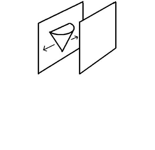
Figure 1: A cartoon of a wave moving into the bulk and along the brane due to a bubble-nucleation event on a brane. The equations in the text provide an approximate description far from the nucleation site, and near the brane (where the disturbance is approximately a plane wave moving parallel to a brane direction).

This type of linearized calculation is not really satisfactory because it models the brane tension as changing simultaneously throughout the brane volume. However causality implies that such a transition must occur locally with the nucleation of a small region having the new tension at some position on the brane, with the region of new tension then expanding to fill space to take more and more of the brane volume to the new vacuum. The resulting geometry is likely to be reasonably complicated, with a wave propagating out into the bulk as well as along the brane directions (see Fig. 1). We expect the scaling solutions of ref. [29, 30] to be obtained after the wave reflects back and forth a sufficient number of times around the internal dimensions.

The solutions in this paper provide some approximate insight into the nature of the waves which would carry the news of the phase transition across the brane and the bulk. The insight is only approximate partly because the wave solutions we consider are plane waves moving along a direction parallel to the branes, rather than describing ‘spherical’ emission into the brane and the bulk from the nucleation event. Our solution might nevertheless capture some of the physics of the outgoing wave far from the nucleation site, along directions in spacetime near to the brane itself (and so moving close to parallel to a brane direction). Since it describes a single wave it also can only apply before any waves have had time to be reflected back to the initial brane after crossing the extra dimensions. In such a situation we expect the physics of wave propagation to be largely insensitive to the specific boundary conditions taken by our solutions on the spectator brane. These conditions need not be inconsistent with one another, particularly in scenarios for which the extra dimensions are much larger than the particle-physics scales which govern the nucleation event itself.

The change in brane properties with wave passage can then be read off from the $u$-dependence of the integration ‘constants’ in the pp-wave solutions. For instance, for the pure-tension branes the quantities $\lambda_{i}(u)$ appearing in eqs. (2.4) can be related to the time-dependent brane stress-energies by formulae such as those given in refs. [39, 29], with the result that the 4D tension of the brane located at $\eta\to\pm\infty$ is proportional to the quantity $3\,\alpha_{\pm}+\beta_{\pm}$, where

$$\alpha_{\pm}(u)=\frac{\lambda_{2}(u)-\lambda_{1}(u)}{5\lambda_{2}(u)-\lambda_{1}(u)\mp 2\lambda_{3}(u)}\quad\hbox{and}\quad\beta_{\pm}(u)=\frac{\lambda_{2}(u)+3\lambda_{1}(u)\mp 2\lambda_{3}(u)}{5\lambda_{2}(u)-\lambda_{1}(u)\mp 2\lambda_{3}(u)}\,.$$ (56)

4 Conclusions

Six dimensional supergravity provides a fruitful laboratory for investigating the issues which underly higher-dimensional physics in general, and brane approaches to the cosmological constant problem in particular. It does so because 6D is rich enough to exhibit many of the properties of still-higher dimensions — like moduli-stabilization through fluxes [41], brane back-reaction on internal geometries, chiral fermions and Green-Schwarz anomaly cancellation [42]. Yet it is also on the one hand simple enough to allow the development of techniques for obtaining physically interesting exact solutions, but on the other hand not so simple as to be misleading about what happens in higher dimensional (in a way which co-dimension one physics sometimes can be).

We have used these properties to explore solution-generation techniques which we believe to be applicable to a wide variety of higher-dimensional supergravities. We do so by using these techniques to construct a new class of time-dependent exact solutions to the field equations of 6D chiral gauged supergravity. These solutions describe the physics of nonlinear gravitational waves passing through compactified spacetimes for which two dimensions are self-consistently compactified in response to the presence of two space-filling branes and a bulk Maxwell flux.

We believe these methods to merit more detailed exploration.

References

- [1] For a survey of many of the higher-dimensional supergravities see, for example, Supergravities in Diverse Dimensions Vols. I & II, ed. by A. Salam and E. Sezgin, World Scientific 1989.
- [2] M. Gutperle and A. Strominger, “Spacelike Branes,” JHEP 0204 (2002) 018 [hep-th/0202210]; C. P. Burgess, F. Quevedo, S. J. Rey, G. Tasinato and I. Zavala, “Cosmological spacetimes from negative tension brane backgrounds,” JHEP 0210 (2002) 028 [hep-th/0207104]; N. Ohta, “Accelerating cosmologies from S-branes,” Phys. Rev. Lett. 91 (2003) 061303 [hep-th/0303238]; C. P. Burgess, C. Nunez, F. Quevedo, G. Tasinato and I. Zavala, “General brane geometries from scalar potentials: Gauged supergravities and accelerating universes,” JHEP 0308 (2003) 056 [hep-th/0305211]; C. M. Chen, P. M. Ho, I. P. Neupane, N. Ohta and J. E. Wang, “Hyperbolic Space Cosmologies,” JHEP 0310 (2003) 058 [hep-th/0306291]; L. Cornalba and M. S. Costa, “Time-dependent orbifolds and string cosmology,” Fortsch. Phys. 52 (2004) 145 [hep-th/0310099]; M. Cariglia, G. W. Gibbons, R. Guven and C. N. Pope, “Non-Abelian pp-waves in D = 4 supergravity theories,” Class. Quant. Grav. 21 (2004) 2849 [hep-th/0312256]; G. Tasinato, I. Zavala, C. P. Burgess and F. Quevedo, “Regular S-brane backgrounds,” JHEP 0404 (2004) 038 [hep-th/0403156]; P. Chen, K. Dasgupta, K. Narayan, M. Shmakova and M. Zagermann, “Brane inflation, solitons and cosmological solutions: I,” JHEP 0509 (2005) 009 [hep-th/0501185]; E. A. Bergshoeff, A. Collinucci, D. Roest, J. G. Russo and P. K. Townsend, “Cosmological D-instantons and cyclic universes,” Class. Quant. Grav. 22 (2005) 2635 [hep-th/0504011]; M. Cvetic, G. W. Gibbons, H. Lu and C. N. Pope, “Rotating Black Holes In Gauged Supergravities: Thermodynamics, Supersymmetric Limits, Topological Solitons And Time Machines,” [hep-th/0504080]; S. Hellerman and I. Swanson, “Cosmological unification of string theories,” arXiv:hep-th/0612116. S. Hellerman and I. Swanson, “Cosmological solutions of supercritical string theory,” arXiv:hep-th/0611317.
- [3] P. K. Townsend and M. N. R. Wohlfarth, “Accelerating cosmologies from compactification,” Phys. Rev. Lett. 91 (2003) 061302 [hep-th/0303097]; S. B. Giddings and R. C. Myers, “Spontaneous decompactification,” Phys. Rev. D 70 (2004) 046005 [hep-th/0404220]; G. W. Gibbons, H. Lu, D. N. Page and C. N. Pope, “Rotating black holes in higher dimensions with a cosmological constant,” Phys. Rev. Lett. 93 (2004) 171102 [hep-th/0409155].
- [4] L. Randall and R. Sundrum, “A large mass hierarchy from a small extra dimension,” Phys. Rev. Lett. 83 (1999) 3370 [hep-ph/9905221]; “An alternative to compactification,” Phys. Rev. Lett. 83 (1999) 4690 [hep-th/9906064].
- [5] Y. Aghababaie, C.P. Burgess, S. Parameswaran and F. Quevedo, Nucl. Phys. B680 (2004) 389–414, [hep-th/0304256]; C. P. Burgess, “Towards a natural theory of dark energy: Supersymmetric large extra dimensions,” AIP Conf. Proc. 743 (2005) 417 [hep-th/0411140].
- [6] Y. Aghababaie et al., “Warped brane worlds in six dimensional supergravity,” JHEP 0309, 037 (2003) [arXiv:hep-th/0308064].
- [7] C.P. Burgess, “Supersymmetric Large Extra Dimensions and the Cosmological Constant: An Update,” Ann. Phys. 313 (2004) 283-401 [hep-th/0402200]; J. Garriga and M. Porrati, “Football shaped extra dimensions and the absence of self-tuning,” JHEP 0408 (2004) 028 [hep-th/0406158].
- [8] C. P. Burgess and D. Hoover, “UV sensitivity in supersymmetric large extra dimensions: The Ricci-flat case,” [hep-th/0504004]; D. M. Ghilencea, D. Hoover, C. P. Burgess and F. Quevedo, “Casimir energies for 6D supergravities compactified on T(2)/Z(N) with Wilson lines,” JHEP 0509, 050 (2005) [hep-th/0506164]; D. Hoover and C. P. Burgess, “Ultraviolet sensitivity in higher dimensions,” JHEP 0601, 058 (2006) [hep-th/0507293].
- [9] G. Azuelos, P. H. Beauchemin and C. P. Burgess, “Phenomenological constraints on extra-dimensional scalars,” J. Phys. G 31, 1 (2005) [hep-ph/0401125]; C. P. Burgess, J. Matias and F. Quevedo, “MSLED: A minimal supersymmetric large extra dimensions scenario,” Nucl. Phys. B 706 (2005) 71 [hep-ph/0404135]; P. H. Beauchemin, G. Azuelos and C. P. Burgess, “Dimensionless coupling of bulk scalars at the LHC,” J. Phys. G 30, N17 (2004) [hep-ph/0407196]; J. Matias and C. P. Burgess, “MSLED, neutrino oscillations and the cosmological constant,” JHEP 0509 (2005) 052 [hep-ph/0508156]; P. Callin and C. P. Burgess, “Deviations from Newton’s law in supersymmetric large extra dimensions,” [hep-ph/0511216].
- [10] N. Arkani-Hamed, S. Dimopoulos, N. Kaloper and R. Sundrum, “A small cosmological constant from a large extra dimension,” Phys. Lett. B 480 (2000) 193, [hep-th/0001197]; S. Kachru, M. B. Schulz and E. Silverstein, “Self-tuning flat domain walls in 5d gravity and string theory,” Phys. Rev. D 62 (2000) 045021, [hep-th/0001206].
-
[11]
S. Forste, Z. Lalak, S. Lavignac and H. P. Nilles, “A comment on
self-tuning and vanishing cosmological constant in the brane
world”, Phys. Lett. B 481 (2000) 360, hep-th/0002164;
JHEP 0009 (2000) 034, [hep-th/0006139];
C. Csaki, J. Erlich, C. Grojean and T.J. Hollowood, “General Properties of the Self-Tuning Domain Wall Approach to the Cosmological Constant Problem,” Nucl. Phys. B584 (2000) 359-386, [hep-th/0004133];
C. Csaki, J. Erlich and C. Grojean, “Gravitational Lorentz Violations and Adjustment of the Cosmological Constant in Asymmetrically Warped Spacetimes,” Nucl. Phys. B604 (2001) 312-342, [hep-th/0012143];
J.M. Cline and H. Firouzjahi, “No-Go Theorem for Horizon-Shielded Self-Tuning Singularities”, Phys. Rev. D65 (2002) 043501, [hep-th/0107198]. - [12] J.-W. Chen, M.A. Luty and E. Pontón, JHEP 0009 (2000) 012, [hep-th/0003067]; S. M. Carroll and M. M. Guica, “Sidestepping the cosmological constant with football-shaped extra dimensions,” [hep-th/0302067]; I. Navarro, “Co-dimension two compactifications and the cosmological constant problem,” JCAP 0309 (2003) 004 [hep-th/0302129]. J. M. Schwindt and C. Wetterich, “Dark energy cosmologies for codimension-two branes,” Nucl. Phys. B 726, 75 (2005) [arXiv:hep-th/0501049]. J. M. Schwindt and C. Wetterich, “The cosmological constant problem in codimension-two brane models,” Phys. Lett. B 628, 189 (2005) [arXiv:hep-th/0508065].
- [13] I. Navarro, “Spheres, deficit angles and the cosmological constant,” Class. Quant. Grav. 20 (2003) 3603 [hep-th/0305014]; H. P. Nilles, A. Papazoglou and G. Tasinato, “Selftuning and its footprints,” Nucl. Phys. B 677 (2004) 405 [hep-th/0309042]; P. Bostock, R. Gregory, I. Navarro and J. Santiago, “Einstein gravity on the Co-dimension 2 brane?,” Phys. Rev. Lett. 92, 221601 (2004) [hep-th/0311074]; J. Vinet and J. M. Cline, “Can Co-dimension-two branes solve the cosmological constant problem?,” Phys. Rev. D 70 (2004) 083514 [hep-th/0406141]; M. L. Graesser, J. E. Kile and P. Wang, “Gravitational perturbations of a six dimensional self-tuning model,” Phys. Rev. D 70 (2004) 024008 [hep-th/0403074]; G. Kofinas, “On braneworld cosmologies from six dimensions, and absence thereof,” [hep-th/0506035].
- [14] C. P. Burgess, “Extra Dimensions and the Cosmological Constant Problem,” arXiv:0708.0911 [hep-ph].
- [15] A. Salvio, “4D effective theory and geometrical approach,” AIP Conf. Proc. 881, 58 (2007) [arXiv:hep-th/0609050]. S. L. Parameswaran, S. Randjbar-Daemi and A. Salvio, Nucl. Phys. B 767, 54 (2007) [arXiv:hep-th/0608074]. A. Salvio, arXiv:hep-th/0701020. M. Peloso, L. Sorbo and G. Tasinato, Phys. Rev. D 73, 104025 (2006) [arXiv:hep-th/0603026]. T. Kobayashi and Y. i. Takamizu, “Hybrid compactifications and brane gravity in six dimensions,” arXiv:0707.0894 [hep-th]. M. Gogberashvili, P. Midodashvili and D. Singleton, “Fermion Generations from ‘Apple-Shaped’ Extra Dimensions,” arXiv:0706.0676 [hep-th]. H. M. Lee and A. Papazoglou, “Gravitino in six-dimensional warped supergravity,” arXiv:0705.1157 [hep-th]. E. Elizalde, M. Minamitsuji and W. Naylor, “Casimir effect in rugby-ball type flux compactifications,” Phys. Rev. D 75, 064032 (2007) [arXiv:hep-th/0702098]. M. Cvetic, G. W. Gibbons and C. N. Pope, “A string and M-theory origin for the Salam-Sezgin model,” Nucl. Phys. B 677, 164 (2004) [arXiv:hep-th/0308026].
- [16] R. Geroch and J. H. Traschen, “Strings and Other Distributional Sources in General Relativity,” Phys. Rev. D 36, 1017 (1987). J. M. Cline, J. Descheneau, M. Giovannini and J. Vinet, “Cosmology of codimension-two braneworlds,” JHEP 0306, 048 (2003) [arXiv:hep-th/0304147]. C. de Rham and A. J. Tolley, “Gravitational waves in a codimension two braneworld,” JCAP 0602, 003 (2006) [arXiv:hep-th/0511138]. S. Fujii, T. Kobayashi and T. Shiromizu, “Low energy effective theory on a regularized brane in six-dimensional flux compactifications,” arXiv:0708.2534 [hep-th]. E. Papantonopoulos, A. Papazoglou and V. Zamarias, “Regularization of conical singularities in warped six-dimensional compactifications,” JHEP 0703, 002 (2007) [arXiv:hep-th/0611311]. E. Papantonopoulos, A. Papazoglou and V. Zamarias, “Induced cosmology on a regularized brane in six-dimensional flux compactification,” arXiv:0707.1396 [hep-th]. M. Minamitsuji and D. Langlois, “Cosmological evolution of regularized branes in 6D warped flux compactifications,” arXiv:0707.1426 [hep-th]. B. Himmetoglu and M. Peloso, “Isolated Minkowski vacua, and stability analysis for an extended brane in the rugby ball,” Nucl. Phys. B 773, 84 (2007) [arXiv:hep-th/0612140].
- [17] W. D. Goldberger and M. B. Wise, Phys. Rev. D 65 (2002) 025011 [arXiv:hep-th/0104170]. C. de Rham, “The Effective Field Theory of Codimension-two Branes,” JHEP 0801, 060 (2008) [arXiv:0707.0884 [hep-th]]. C. de Rham, “Classical Renormalization of Codimension-two Brane Couplings,” AIP Conf. Proc. 957, 309 (2007) [arXiv:0710.4598 [hep-th]].
- [18] H. Nishino and E. Sezgin, Phys. Lett. 144B (1984) 187; “The Complete N=2, D = 6 Supergravity With Matter And Yang-Mills Couplings,” Nucl. Phys. B278 (1986) 353; S. Randjbar-Daemi, A. Salam, E. Sezgin and J. Strathdee, Phys. Lett. B151 (1985) 351; A. Salam and E. Sezgin, “Chiral Compactification On Minkowski Of N=2 Einstein-Maxwell Supergravity In Six-Dimensions,” Phys. Lett. B 147 (1984) 47.
- [19] Other 6D supergravities are discussed in N. Marcus and J.H. Schwarz, Phys. Lett. B 115 (1982) 111; R. D’Auria, P. Fre and T. Regge, “Consistent Supergravity In Six-Dimensions Without Action Invariance,” Phys. Lett. B 128 (1983) 44; Y. Tanii, “N=8 Supergravity In Six-Dimensions,” Phys. Lett. B 145 (1984) 197; L.J. Romans, Nucl. Phys. B269 (1986) 691–711.
- [20] S. Weinberg, Gravitation and Cosmology, Wiley, New York, 1972.
- [21] C.W. Misner, K.P. Thorne and J.A. Wheeler, Gravitation, W.H. Freeman and Company (1970).
- [22] G. W. Gibbons, R. Guven and C. N. Pope, “3-branes and uniqueness of the Salam-Sezgin vacuum,” Phys. Lett. B 595, 498 (2004) [hep-th/0307238].
- [23] C. P. Burgess, F. Quevedo, G. Tasinato and I. Zavala, “General axisymmetric solutions and self-tuning in 6D chiral gauged supergravity,” JHEP 0411, 069 (2004) [hep-th/0408109].
- [24] S. Randjbar-Daemi and E. Sezgin, “Scalar potential and dyonic strings in 6d gauged supergravity,” Nucl. Phys. B 692 (2004) 346 [hep-th/0402217]; A. Kehagias, “A conical tear drop as a vacuum-energy drain for the solution of the cosmological constant problem,” Phys. Lett. B 600 (2004) 133 [hep-th/0406025]; S. Randjbar-Daemi and V. A. Rubakov, “4d-flat compactifications with brane vorticities,” JHEP 0410, 054 (2004) [hep-th/0407176]; H. M. Lee and A. Papazoglou, “Brane solutions of a spherical sigma model in six dimensions,” Nucl. Phys. B 705 (2005) 152 [hep-th/0407208]; V. P. Nair and S. Randjbar-Daemi, “Nonsingular 4d-flat branes in six-dimensional supergravities,” JHEP 0503 (2005) 049 [hep-th/0408063]; S. L. Parameswaran, G. Tasinato and I. Zavala, “The 6D SuperSwirl,” [hep-th/0509061]; H. M. Lee and C. Ludeling, “The general warped solution with conical branes in six-dimensional supergravity,” [hep-th/0510026].
- [25] A. Tolley, C.P. Burgess, D. Hoover and Y. Aghababaie, “Bulk Singularities and the Effective Cosmological Constant for Higher Co-dimension Branes,” JHEP 0603 (2006) 091 [hep-th/0512218].
- [26] J. M. Cline, J. Descheneau, M. Giovannini and J. Vinet, “Cosmology of codimension-two braneworlds,” JHEP 0306, 048 (2003) [arXiv:hep-th/0304147]. H. M. Lee and A. Papazoglou, “Scalar mode analysis of the warped Salam-Sezgin model,” [hep-th/0602208];
- [27] C. P. Burgess, C. de Rham, D. Hoover, D. Mason and A. J. Tolley, “Kicking the rugby ball: Perturbations of 6D gauged chiral supergravity,” JCAP 0702, 009 (2007) [arXiv:hep-th/0610078].
- [28] S. L. Parameswaran, S. Randjbar-Daemi and A. Salvio, “Stability and Negative Tensions in 6D Brane Worlds,” arXiv:0706.1893 [hep-th].
- [29] A. J. Tolley, C. P. Burgess, C. de Rham and D. Hoover, “Scaling solutions to 6D gauged chiral supergravity,” New J. Phys. 8, 324 (2006) [arXiv:hep-th/0608083].
- [30] E. J. Copeland and O. Seto, “Dynamical solutions of warped six dimensional supergravity,” arXiv:0705.4169 [hep-th]. T. Kobayashi and M. Minamitsuji, “Brane cosmological solutions in six-dimensional warped flux compactifications,” arXiv:0705.3500 [hep-th].
- [31] H. Stephani, D. Kramer, M. MacCallum, C. Hoenselaers and E. Herlt, “Exact solutions of Einstein’s field equations,” Cambridge, UK: Univ. Pr. (2003) 701 P
- [32] N. Kaloper and D. Kiley, “Exact black holes and gravitational shockwaves on codimension-2 branes,” JHEP 0603, 077 (2006) [arXiv:hep-th/0601110]. M. Anber and L. Sorbo, “Two gravitational shock waves on the AdS3 brane,” arXiv:0706.1560 [hep-th]. N. Kaloper, “Gravitational shock waves and their scattering in brane-induced gravity,” Phys. Rev. D 71, 086003 (2005) [Erratum-ibid. D 71, 129905 (2005)] [arXiv:hep-th/0502035]. N. Kaloper, “Brane-induced gravity’s shocks,” Phys. Rev. Lett. 94, 181601 (2005) [Erratum-ibid. 95, 059901 (2005)] [arXiv:hep-th/0501028]. D. Kiley, “Rotating Black Holes on Codimension-2 Branes,” arXiv:0708.1016 [hep-th].
- [33] A. A. Coley, “Classification of the Weyl Tensor in Higher Dimensions and Applications,” arXiv:0710.1598 [gr-qc]. A. Coley, A. Fuster and S. Hervik, “Supergravity solutions with constant scalar invariants,” arXiv:0707.0957 [hep-th]. A. A. Coley, A. Fuster, S. Hervik and N. Pelavas, “Vanishing Scalar Invariant Spacetimes in Supergravity,” JHEP 0705, 032 (2007) [arXiv:hep-th/0703256]. A. Coley, A. Fuster, S. Hervik and N. Pelavas, “Higher dimensional VSI spacetimes,” Class. Quant. Grav. 23, 7431 (2006) [arXiv:gr-qc/0611019]. A. Coley, R. Milson, V. Pravda and A. Pravdova, “Vanishing scalar invariant spacetimes in higher dimensions,” Class. Quant. Grav. 21, 5519 (2004) [arXiv:gr-qc/0410070]. A. A. Coley and S. Hervik, “Brane waves,” Class. Quant. Grav. 21, 5759 (2004) [arXiv:gr-qc/0405089]. A. Coley, R. Milson, V. Pravda and A. Pravdova, “Classification of the Weyl tensor in higher-dimensions,” Class. Quant. Grav. 21, L35 (2004) [arXiv:gr-qc/0401008].
- [34] J. B. Griffiths, “Colliding plane waves in general relativity,” Oxford, UK: Clarendon (1991) 232 p. (Oxford mathematical monographs). D. M. Eardley and S. B. Giddings, “Classical black hole production in high-energy collisions,” Phys. Rev. D 66, 044011 (2002) [arXiv:gr-qc/0201034]. N. Kaloper and J. Terning, “How black holes form in high energy collisions,” Gen. Rel. Grav. 39, 1525 (2007) [arXiv:0705.0408 [hep-th]].
- [35] J. M. Maldacena, “Lectures on AdS/CFT,” arXiv:hep-th/0309246. A. Pankiewicz, “Strings in plane wave backgrounds,” Fortsch. Phys. 51, 1139 (2003) [arXiv:hep-th/0307027].
- [36] A. J. Tolley, “String propagation through a big crunch / big bang transition,” Phys. Rev. D 73, 123522 (2006) [arXiv:hep-th/0505158].
- [37] G. T. Horowitz and A. R. Steif, “Strings in strong gravitational fields,” Phys. Rev. D 42, 1950 (1990). G. T. Horowitz and A. R. Steif, “Space-Time Singularities in String Theory,” Phys. Rev. Lett. 64, 260 (1990).
- [38] M. Blau and M. O’Loughlin, “Homogeneous plane waves,” Nucl. Phys. B 654, 135 (2003) [arXiv:hep-th/0212135]. M. Blau, M. O’Loughlin, G. Papadopoulos and A. A. Tseytlin, “Solvable models of strings in homogeneous plane wave backgrounds,” Nucl. Phys. B 673, 57 (2003) [arXiv:hep-th/0304198].
- [39] I. Navarro and J. Santiago, “Gravity on Co-dimension 2 brane worlds,” JHEP 0502, 007 (2005) [hep-th/0411250].
- [40] G. W. Gibbons and C. N. Pope, “Consistent S**2 Pauli reduction of six-dimensional chiral gauged Einstein-Maxwell supergravity,” Nucl. Phys. B 697 (2004) 225 [hep-th/0307052].
- [41] Y. Aghababaie, C. P. Burgess, S. L. Parameswaran and F. Quevedo, “Susy Breaking and Moduli Stabilization from Fluxes in Gauged 6D Supergravity,” JHEP 0303 (2003) 032 [hep-th/0212091].
-
[42]
M.B. Green, J.H. Schwarz and P.C. West, Nucl. Phys. B254 (1985) 327;
J. Erler, J. Math. Phys. 35 (1994) 1819 [hep-th/9304104]. - [43] C. P. Burgess, D. Hoover and G. Tasinato, “UV Caps and Modulus Stabilization for 6D Gauged Chiral Supergravity,” JHEP 0709, 124 (2007) [arXiv:0705.3212 [hep-th]].
- [44] P. C. Aichelburg and R. U. Sexl, “On the Gravitational field of a massless particle,” Gen. Rel. Grav. 2 (1971) 303.