A Deterministic Approach to
Wireless Relay Networks

Abstract

We present a deterministic channel model which captures several key features of multiuser wireless communication. We consider a model for a wireless network with nodes connected by such deterministic channels , and present an exact characterization of the end-to-end capacity when there is a single source and a single destination and an arbitrary number of relay nodes. This result is a natural generalization of the max-flow min-cut theorem for wireline networks. Finally to demonstrate the connections between deterministic model and Gaussian model, we look at two examples: the single-relay channel and the diamond network. We show that in each of these two examples, the capacity-achieving scheme in the corresponding deterministic model naturally suggests a scheme in the Gaussian model that is within 1 bit and 2 bit respectively from cut-set upper bound, for all values of the channel gains. This is the first part of a two-part paper; the sequel [1] will focus on the proof of the max-flow min-cut theorem of a class of deterministic networks of which our model is a special case.

I Introduction

Two fundamental features distinguish wireless communication from wireline communication:

• first, the broadcast nature of wireless communication; wireless users communicate over the air and signals from any one transmitter is heard by multiple nodes with possibly different signal strengths.

• second, the superposition nature; a wireless node receives signals from multiple simultaneously transmitting nodes, with the received signals all superimposed on top of each other.

Because of these two effects, links in a wireless network are never isolated but instead interact in seemingly complex ways. This is quite unlike the wired world where each transmitter-receiver pair can often be thought of as isolated point-to-point links.

The multiuser Gaussian channel model is the standard one used in information theory to capture these two effects: signals get attenuated by complex gains and added together with Gaussian noise at each receiver (the Gaussian noises at different receivers being independent of each other.). Unfortunately, except for the simplest networks such as the one-to-many Gaussian broadcast channel and the many-to-one Gaussian multiple access channel, the capacity region of most Gaussian networks is unknown. For example, even the capacity of the simplest Gaussian relay network, with a single source, single destination and single relay, is an open question.

To make further progress, in this paper we present a new multiuser channel model which is analytically simpler than Gaussian models but yet still captures the two key features of wireless communication of broadcast and superposition. The key feature of this model is that the channels are deterministic: the signal received at a node in the network is a (deterministic) function of the transmitted signals. This model is a good approximation of the corresponding multiuser Gaussian model under two assumptions that are quite common in many wireless communication scenarios:

• the additive noise at each receiver is small compared to the strength of the signals received from the transmitters (high SNR regime)

• the signals from different nodes in the network can be received at very different power at a given receiver (high dynamic range of received signals)

Essentially, this class of deterministic models allow us to focus on the interaction between the signals transmitted from the different nodes of the network rather than the noise. In this paper we first introduce and motivate the deterministic model through three basic examples: point-to-point, broadcast and multiple-access channels. Then we consider a network with a single source and a single destination but with arbitrary number of relay nodes, all connected by such deterministic channels. The cut-set bound on the end-to-end capacity of such networks can actually be achieved, the proof of which can be found in the sequel [1]. Finally to demonstrate the connections between deterministic model and Gaussian model, we look at two examples: The single relay channel and the Diamond network. We show that the capacity-achieving schemes in the corresponding deterministic model naturally suggest schemes whose performance is ”close” to the cut-set upper bound in the Gaussian model. More specifically, we show that in the single-relay network, the gap is at most 1 bit/s/Hz, and in the Diamond network, the gap is at most 2 bit/s/Hz. The gaps hold for all values of the channel gains and are relevant particularly when the SNR is high and the capacity is large.

II A Deterministic Model for Wireless Networks

In this section we introduce a deterministic model for wireless networks. First we motivate this model by looking at the following three examples:

1. Point-to-point channel

2. Broadcast Channel (BC)

3. Multiple access channel (MAC)

Through each example we will discuss how the proposed deterministic model captures the fundamental aspects of wireless channels.

II-A Point-to-Point

Consider an AWGN channel,

$$y=hx+z$$ (1)

where $z\sim\mathcal{CN}(0,1)$. There is also an average power constraint $E[|x|^{2}]\leq 1$ at the transmitter. In this paper we normalize both transmit power and noise power to be equal to 1 and capture the signal-to-noise ratio (${\sf SNR}$) in terms of channel gains. So we model $h$ as a fixed number representing the channel gain, hence

$$h=\sqrt{{\sf SNR}}$$ (2)

It is well known that the capacity of this point-to-point channel is

$$C_{\text{AWGN}} = \log\left(1+{\sf SNR}\right)$$ (3)

To get an intuitive understanding of this capacity formula lets write the received signal in equation (1), $y$, in terms of binary expansions of $x$ and $z$. For simplicity assume $x$ and $z$ are real numbers, then we have

$$y=2^{\frac{1}{2}\log{\sf SNR}}\sum_{i=1}^{\infty}x(i)2^{-i}+\sum_{i=-\infty}^{\infty}z(i)2^{-i}$$ (4)

To simplify the effect of background noise assume it has a peak power equal to 1. Then we can write

$$y = 2^{\frac{1}{2}\log{\sf SNR}}\sum_{i=1}^{\infty}x(i)2^{-i}+\sum_{i=1}^{\infty}z(i)2^{-i}$$ (5)

or,

$$y\approx 2^{n}\sum_{i=1}^{n}x(i)2^{-i}+\sum_{i=1}^{\infty}\left(x(i+n)+z(i)\right)2^{-i}$$ (6)

where $n=\lceil\frac{1}{2}\log{\sf SNR}\rceil$. Therefore if we just ignore the 1 bit of the carry-over from the second summation ($\sum_{i=1}^{\infty}\left(x(i+n)+z(i)\right)2^{-i}$) to the first summation ($2^{n}\sum_{i=1}^{n}x(i)2^{-i}$) we can intuitively model a point-to-point Gaussian channel as a pipe that truncates the transmitted signal and only passes the bits that are above noise level. Therefore think of transmitted signal $x$ as a sequence of bits at different signal levels, with the highest signal level in $x$ being the most significant bit (MSB) and the lowest level being the least significant bit (LSB). In this simplified model the receiver can see the $n$ most significant bits of $x$ without any noise and the rest are not seen at all. Clearly there is a correspondence between $n$ and ${\sf SNR}$ in dB scale,

$$n\leftrightarrow\lceil\log{\sf SNR}\rceil$$ (7)

note that a factor of $\frac{1}{2}$ is needed in the case of AWGN channel with real signals rather than complex signals. As we notice in this simplified model there is no background noise any more and hence we call it a deterministic model. Pictorially the deterministic model corresponding to the AWGN channel is shown in figure 1. In this figure at the transmitter there are several small circles. Each circle represents a signal level and a binary digit can be put for transmission at each signal level. Depending on $n$, which represents the channel gain in dB scale, the transmitted bits at first $n$ signal levels will be received clearly at the destination. However the bits at other signal levels will not go through the channel. In analogy to the AWGN channel the first $n$ bits are those that are above noise level and the remaining are the ones that are below noise level. Therefore if transmit signal, $\mathbf{x}$, is a binary vector of length $q$, then deterministic channel only delivers its first $n$ elements to the destination. We can algebraically write this input-output relationship by shifting $\mathbf{x}$ down by $q-n$ elements or more precisely

$$\mathbf{y}={\bf S^{q-n}}\mathbf{x}$$ (8)

where $\mathbf{x}$ and $\mathbf{y}$ are binary vectors of length $q$ denoting transmit and received signals respectively and ${\bf S}$ is the $q\times q$ shift matrix,

$$\mbox{${\bf S}$}=\left(\begin{array}[]{ccccc}0&0&0&\cdots&0\\ 1&0&0&\cdots&0\\ 0&1&0&\cdots&0\\ \vdots&\ddots&\ddots&\ddots&\vdots\\ 0&\cdots&0&1&0\\ \end{array}\right)$$ (9)

\begin{picture}(3854.0,1974.0)(4189.0,-4423.0)\end{picture}

Figure 1: Pictorial representation of the deterministic model for point-to-point channel

Clearly the capacity of this deterministic point-to-point channel is

$$C_{\text{det}}=n$$ (10)

where $n=\lceil\log{\sf SNR}\rceil$. It is interesting to note that this is a within-one-bit approximation of the capacity of the AWGN channel.

II-B Broadcast Channel (BC):

Based on the intuition obtained so far, it is straightforward to think of a deterministic model for the Gaussian broadcast channel. Assume there are only two receivers. The received ${\sf SNR}$ at receiver $i$ is denoted by ${\sf SNR}_{i}$ for $i=1,2$. Without loss of generality assume ${\sf SNR}_{2}\leq{\sf SNR}_{1}$. Consider the binary expansion of the transmitted signal, $x$. Then we can deterministically model the Gaussian BC channel as the following

• Receiver 2 (weak user) receives only the first $n_{2}$ bits in the binary expansion of $x$. Those bits are the ones that arrive above noise level

• Receiver 1 (strong user) receives the first $n_{1}$ ($n_{1}>n_{2}$) bits in the binary expansion of $x$. Clearly these bits contain what receiver 1 gets

Pictorially the deterministic model for a Gaussian BC channel is shown in figure 2 (a). In this particular example $n_{1}=5$ and $n_{2}=2$, therefore both users receive the first two most significant bits of the transmitted signal. However user 1 (strong user) receives additional three bits from the next three signal levels of the transmitted signal. There is also the same correspondence between $n$ and channel gains in dB,

$$n_{i}\leftrightarrow\lceil\log{\sf SNR}_{i}\rceil,\quad i=1,2$$ (11)

To understand how closely we are modeling the Gaussian BC channel, the capacity region of Gaussian BC channel and deterministic BC channel are shown in figure 2 (b). In fact it is easy to verify that these regions are within one bit per user of each other (i.e. if a pair $(R_{1},R_{2})$ is in the capacity region of the deterministic BC then there is a pair within one bit per component of $(R_{1},R_{2})$ that is in the capacity region of the Gaussian BC).

(a) Pictorial representation of the deterministic model for Gaussian BC

(b) Capacity region of Gaussian BC channel (solid line). Capacity region of deterministic BC channel (dashed line)

Figure 2: Pictorial representation of the deterministic model for Gaussian BC is shown in (a). Capacity region of Gaussian and deterministic BC are shown in (b)

II-C Multiple Access Channel (MAC):

Consider a two user Gaussian MAC channel:

$$y=h_{1}x_{1}+h_{2}x_{2}+z$$ (12)

where $z\sim\mathcal{CN}(0,1)$. There is also an average power constraint equal to 1 at both transmitters. The channel gains are

$$h_{i}=\sqrt{{\sf SNR}_{i}},\quad i=1,2$$ (13)

Without loss of generality assume ${\sf SNR}_{2}<{\sf SNR}_{1}$. The capacity region of this channel is well-known to be the set of non-negative pairs $(R_{1},R_{2})$ satisfying

$$R_{i} \leq \log(1+{\sf SNR}_{i}),\quad i=1,2$$ (14)

$$R_{1}+R_{2} \leq \log(1+{\sf SNR}_{1}+{\sf SNR}_{2})$$ (15)

This region is plotted with solid line in figure 3 (b).

To intuitively understand what happens in a Gaussian MAC channel we write the received signal, $y$, in terms of the binary expansions of $x_{1}$, $x_{2}$ and $z$. For simplicity assume $x_{1}$, $x_{2}$ and $z$ are all real numbers, then we have

$$y=2^{\frac{1}{2}\log{\sf SNR}_{1}}\sum_{i=1}^{\infty}x_{1}(i)2^{-i}+2^{\frac{1}{2}\log{\sf SNR}_{2}}\sum_{i=1}^{\infty}x_{2}(i)2^{-i}+\sum_{i=-\infty}^{\infty}z(i)2^{-i}$$ (16)

To simplify the effect of background noise assume it has a peak power equal to 1. Then we can write

$$y=2^{\frac{1}{2}\log{\sf SNR}_{1}}\sum_{i=1}^{\infty}x_{1}(i)2^{-i}+2^{\frac{1}{2}\log{\sf SNR}_{2}}\sum_{i=1}^{\infty}x_{2}(i)2^{-i}+\sum_{i=1}^{\infty}z(i)2^{-i}$$ (17)

or,

$$y \approx 2^{n_{1}}\sum_{i=1}^{n_{1}-n_{2}}x_{1}(i)2^{-i}+2^{n_{2}}\sum_{i=1}^{n_{2}}\left(x_{1}(i+n_{1}-n_{2})+x_{2}(i)\right)2^{-i}$$ (18)

$$+\sum_{i=1}^{\infty}\left(x_{1}(i+n_{1})+x_{2}(i+n_{2})+z(i)\right)2^{-i}$$

where $n_{i}=\lceil\frac{1}{2}\log{\sf SNR}_{i}\rceil$ for $i=1,2$. Therefore based on the intuition obtained from the point-to-point AWGN channel, we can approximately model a MAC channel as follows

• That part of $x_{1}$ that is above ${\sf SNR}_{2}$ ($x_{1}(i)$, $1\leq i\leq n_{1}-n_{2}$) is received clearly without any interference from $x_{2}$

• The remaining part of $x_{1}$ that is above noise level ($x_{1}(i)$, $n_{1}-n_{2}<i\leq n_{1}$) and that part of $x_{2}$ that is above noise level ($x_{1}(i)$, $1\leq i\leq n_{2}$) interact with each other and received without any noise

• Those parts of $x_{1}$ and $x_{2}$ that are below noise level are truncated and not received at all

The key point is how to model the interaction between the bits that are received at the same signal level. In our deterministic model we ignore the carry-over’s of the real addition and we model the interaction by the modulo 2 sum of the bits that are arrived at the same signal level. Pictorially the deterministic model for a Gaussian MAC channel is shown in figure 3 (a). Analogous to the deterministic model for the point-to-point channel, we can write

$$\mathbf{y}={\bf S^{q-n_{1}}}\mathbf{x_{1}}\oplus{\bf S^{q-n_{2}}}\mathbf{x_{2}}$$ (19)

where the summation is in $\mbox{$\mathbb{F}$}_{2}$ (modulo 2). Here $\mathbf{x_{i}}$ ($i=1,2$) and $\mathbf{y}$ are binary vectors of length $q$ denoting transmit and received signals respectively and ${\bf S}$ is a $q\times q$ shift matrix. There is also a relationship between $n_{i}$’s and the channel gain in dB:

$$n_{i}\leftrightarrow\lceil\log{\sf SNR}_{i}\rceil,\quad i=1,2$$ (20)

Note that if one wants to make a connection between the deterministic model and real Gaussian MAC channel (rather than complex) a factor of $\frac{1}{2}$ is necessary.

Now compared to simple point-to-point case we now have interaction between the digits that receive at the same signal level at the receiver. However, we limit the receiver to only observe the modulo 2 summation of those bits that arrive at the same signal level. In some sense this way of modeling interaction is similar to the collision model. In the collision model if two packets arrive simultaneously at a receiver both are dropped, similarly here if two bits arrive simultaneously at the same signal level the receiver gets only their modulo 2 sum, which means it can not figure out any of them. On the other hand, unlike in the simplistic collision model where the entire packet is lost when there is collision, the most significant bits of the stronger user remain intact. This is reminiscent of the familiar capture phenomenon in CDMA systems: the strongest user can be heard even when multiple users simultaneously transmit.

(a) Pictorial representation of the deterministic MAC.

(b) Capacity region of Gaussian MAC. (solid line). Capacity region of deterministic MAC.(dashed line)

Figure 3: Pictorial representation of the deterministic MAC is shown in (a). Capacity region of Gaussian and deterministic MACs are shown in (b)

Now a natural question is how close is the deterministic model to the actual Gaussian model. To answer this question we look at the capacity region of the deterministic MAC. It is easy to verify that the capacity region of the deterministic MAC is the set of non-negative pairs $(R_{1},R_{2})$ satisfying

$$R_{2} \leq n_{2}$$ (21)

$$R_{1}+R_{2} \leq n_{1}$$ (22)

where $n_{i}=\log{\sf SNR}_{i}$ for $i=1,2$. This region is plotted with dashed line in figure 3 (b). In this deterministic model the ”carry-over” from one level to the next that would happen with real addition is ignored. However as we notice still the capacity region is very close to the capacity region of the Gaussian model. In fact it is easy to verify that they are within one bit per user of each other (i.e. if a pair $(R_{1},R_{2})$ is in the capacity region of the deterministic MAC then there is a pair within one bit per component of $(R_{1},R_{2})$ that is in the capacity region of the Gaussian MAC). The intuitive explanation for this is that in real addition once two bounded signals are added together the magnitude increases however, it can only become as large as twice the maximum size of individual ones. Therefore the cardinality size of summation is increased by at most one bit. On the other hand in finite-field addition there is no magnitude associated with signals and the summation is still in the same field size as the individual signals. So the gap between Gaussian and deterministic model for two user MAC is intuitively this one bit of cardinality increase.

II-D The Deterministic Model for General Networks

At this point we are ready to explicitly introduce the deterministic model for general wireless relay networks. We model a wireless network $G$ as a set of nodes $V$, where $|V|=N$.

Communication from node $i$ to node $j$ has a non-negative integer gain $n_{(i,j)}$ associated with it. This number models the channel gain in a corresponding Gaussian setting. At each time $t$, node $i$ transmits a vector ${\bf x_{i}}[t]\in\mbox{$\mathbb{F}$}_{2}^{q}$ and receive a vector ${\bf y_{i}}[t]\in\mbox{$\mathbb{F}$}_{2}^{q}$ where $q=\max_{i,j}(n_{(i,j)})$. The received signal at each node is a deterministic function of the transmitted signals at the other nodes, with the following input-output relation: if the nodes in the network transmit ${\bf x_{1}}[t],{\bf x_{2}}[t],\ldots{\bf x_{N}}[t]$ then the received signal at node j, $1\leq j\leq N$ is:

$${\bf y_{i}}[t]=\sum_{k=1}^{N}{\bf S^{q-n_{k,j}}}{\bf x_{k}}[t]$$ (23)

for all $1\leq k\leq N$ and the summation and multiplication is in $\mbox{$\mathbb{F}$}_{2}$.

The deterministic wireless network can be represented pictorially and an example is illustrated in Figure 4.

Figure 4: Pictorial representation of Deterministic relay network

II-E Related Works

Finite field addition makes the model much more tractable, and neglecting the 1-bit carryover from one level to the next introduce a small error when the SNR is high. Other works [2] have also exploited the simplicity of finite-field addition over real addition. Aref [3] is one of the earliest works that use deterministic models for relay networks, and for which he proved a capacity result for the single-source-single-destination case. However, his model only captures the broadcast aspect but not the superposition aspect. This work was later extended to the multicast setting by Ratnaker and Kramer [4]. Aref and El Gamal [5] also computed the capacity of the semi-determinstic relay channel but only with a single relay. Gupta et al [6] also uses finite-field deterministic addition to model the superposition property, but they do not have the notion of signal scale and the channel as sending some of the signal scales to below noise level. Instead they use random erasures to model noise.

III Single-Source, Single-Destination Network and its Capacity

Given the deterministic model of Section II, we study the information flow for a single source-destination network (unicast).

First we derive the cut-set upper bound on the capacity of this network.

Definition III.1

A cut, $\Omega$ in the deterministic relay network $G$ with two distinguished vertices: the source, $S$, and the destination, $D$, is a split of the vertices into two disjoint sets $\Omega$ and $\Omega^{c}$, such that $S\in\Omega$ and $D\in\Omega^{c}$.

For any cut $\Omega$ we define $\mbox{${\bf G}$}_{\Omega,\Omega^{c}}$ as the incidence matrix associated with the bipartite graph with the small nodes of $\Omega$ on the left side and the small nodes of $\Omega^{c}$ on the right side and with all edges going from small nodes of $\Omega$ to small nodes of $\Omega$ based on the equation described in (23). For example in Figure 4 consider the cut $\Omega$ that separates $\Omega=\{S,A_{1},A_{2}\}$ from $\Omega^{c}=\{B_{1},B_{2},D\}$ then $\mbox{${\bf G}$}_{\Omega,\Omega^{c}}$ is just the incidence matrix of the bipartite graph between the small nodes on $A_{1}$ and $A_{2}$ and the small nodes on $B_{1}$ and $B_{2}$. Therefore

$$\mbox{${\bf G}$}_{\Omega,\Omega^{c}}=\left(\begin{array}[]{cccccccccc}0&0&0&0&0&0&0&0&0&0\\ 0&0&0&0&0&0&0&0&0&0\\ 1&0&0&0&0&0&0&0&0&0\\ 0&1&0&0&0&1&0&0&0&0\\ 0&0&1&0&0&0&1&0&0&0\\ 0&0&0&0&0&0&0&0&0&0\\ 0&0&0&0&0&0&0&0&0&0\\ 0&0&0&0&0&1&0&0&0&0\\ 0&0&0&0&0&0&1&0&0&0\\ 1&0&0&0&0&0&0&1&0&0\\ \end{array}\right)$$ (24)

Equivalently, $\mbox{${\bf G}$}_{\Omega,\Omega^{c}}$ is the transfer matrix from the super vector of all signals transmitted on the nodes in $\Omega$ to the vector of all received signals on the nodes in $\Omega^{c}$.

Now based on the cut-set bound theorem [7] we have,

Lemma III.2

The capacity $C$ of any deterministic wireless network $G$ is upper bounded by

$$C\leq\min_{\Omega}\mathrm{rank}(\mbox{${\bf G}$}_{\Omega,\Omega^{c}})$$ (25)

Proof:

From the cut-set upper bound theorem [7] we have

$$C\leq\max_{p(x_{1},\ldots,x_{n})}\min_{\Omega}I\left(\{x_{i}|i\in\Omega\};\{y_{j}|j\in\Omega^{c}\}|\{x_{i}|i\in\Omega^{c}\}\right)$$ (26)

Since the channels are deterministic we can write this as

$$C\leq\max_{p(x_{1},\ldots,x_{n})}\min_{\Omega}H\left(\{\{y_{j}|j\in\Omega^{c}\}|\{x_{i}|i\in\Omega^{c}\}\right)$$ (27)

Now note that each of these conditional entropies is at most equal to the dimension of the range space of the transfer matrix associated with that cut, achieved when the conditional output is uniformly distributed over its possible values. Now by properties of finite-field arithmetic, this can be simultaneously achieved for all conditional entropies by choosing independent and uniform distribution of $x_{i}$’s in $\mbox{$\mathbb{F}$}_{2}^{q}$. Hence, the cut-set bound can be expressed in terms of the minimum rank of the transfer matrices associated with the cuts. ∎

Now the following main theorem states that the capacity of the wireless deterministic network is equal to its cut-set bound.

Theorem III.3

If $G$ is a deterministic wireless network the cooperative capacity of this network from $S$ to $D$ denoted by $C$ is equal to

$$C=\min_{\Omega}\mathrm{rank}(\mbox{${\bf G}$}_{\Omega,\Omega^{c}})$$ (28)

where the minimum is taken over all cuts in $G$.

Proof:

The proof of this result can be found in the sequel [1] to this paper. ∎

For the example shown in Figure 4 the theorem states that the capacity of this wireless deterministic network is equal to $5$ which is the value of the cut with $\Omega=\{S,A_{1}\}$ and $\Omega^{c}=\{A_{2},B_{1},B_{2},D\}$. Note that there are several other tight cuts such as $\Omega=\{S\}$ and $\Omega^{c}=\{A_{1},A_{2},B_{1},B_{2},D\}$.

For wireline networks with unit-capacity edges, the classic max-flow min-cut theorem says that the maximum achievable rate from source to destination is equal to the minimum of the values of the cuts, where the value of a cut is the number of edges crossing it. Theorem III.3 can be viewed as an analogy of this result for our deterministic model, with the cut value being the rank of the transfer matrix. In fact, both the wireline model and our deterministic model are special cases of a more general class of linear deterministic models, where the matrix ${\bf S^{q-n_{k,j}}}$ in equation (23) is replaced by a general binary matrix ${\bf G_{k,j}}$. The analysis of this class of model is the focus of [1], and the main result there is a generalization of both the classic max-flow min-cut theorem and Theorem III.3.

IV Connections to Gaussian Relay Networks

In this section we will discuss some connections between the deterministic model and the Gaussian model. We will look at two examples of Gaussian relay networks. In these examples we will show that a capacity-achieving scheme in the corresponding deterministic model naturally suggests a scheme in the Gaussian network that achieves a rate whose gap from its cut-set upper bound is bounded independent of the values of the channel gains. Therefore we have uniformly good approximation of the capacities of these relay networks, uniform over all values of the channel gains.

IV-A Relay channel to within one bit

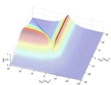
Figure 5: The gap between cut-set upper bound and achievable rate of decode-forward scheme in Gaussian relay channel

In this section we look at a simple Gaussian network with only one relay. The capacity of this network has been an open problem for several decades. Here we will use the deterministic model to find a near-optimal communication scheme for this network. First we build the corresponding deterministic model of this relay channel with channel gains denoted by $n_{SR}$, $n_{SD}$ and $n_{RD}$. From theorem III.3 we know that the capacity of this deterministic channel is equal to

$$C_{relay}^{d} = \min\left(\max(n_{SR},n_{SD}),\max(n_{RD},n_{SD})\right)$$ (29)

$$= n_{SD}+\min\left((n_{SR}-n_{SD})^{+},(n_{RD}-n_{SD})^{+}\right)~{}$$ (30)

Note that equation (30) naturally implies a capacity-achieving scheme for this deterministic relay network: First $n_{SD}$ bits are sent from the source directly to the destination; then, the remaining $\min\left((n_{SR}-n_{SD})^{+},(n_{RD}-n_{SD})^{+}\right)$ bits can be routed on the non-interfering signal levels from the source to the relay and then to the destination. This suggests a decode-and-forward scheme for the original Gaussian relay channel. If $|h_{SR}|<|h_{SD}|$ then the relay is ignored and a communication rate equal to $R=\log(1+|h_{SD}|^{2})$ is achievable. If $|h_{SR}|>|h_{SD}|$ the problem becomes more interesting. In this case we can think of a decode-forward scheme as described in [10]. Then by using a block-Markov encoding scheme the following communication rate is achievable:

$$R=\min\left(\log\left(1+|h_{SR}|^{2}\right),\log\left(1+|h_{SD}|^{2}+|h_{RD}|^{2}\right)\right)$$ (31)

Therefore overall the following rate is always achievable:

$$R_{\text{DF}}=\max\{\log(1+|h_{SD}|^{2}),\quad\quad\quad\quad\quad\quad$$

$$\min\left(\log\left(1+|h_{SR}|^{2}\right),\log\left(1+|h_{SD}|^{2}+|h_{RD}|^{2}\right)\right)\}$$ (32)

Now we show that the achievable rate of this communication scheme is within one bit of the cut-set upper bound of this network for all channel gains. To do so we should compare this achievable rate by the cut-set upper bound on the capacity of the Gaussian relay network,

$$C \leq \overline{C}=\max_{|\rho|\leq 1}\min\{\log\left(1+(1-\rho^{2})(|h_{SD}|^{2}+|h_{SR}|^{2})\right),$$ (33)

$$,\log\left(1+|h_{SD}|^{2}+|h_{RD}|^{2}+2\rho|h_{SD}||h_{RD}|\right)\}$$

Note that if $|h_{SR}|>|h_{SD}|$ then

$$R_{DF}=\min\left(\log\left(1+|h_{SR}|^{2}\right),\log\left(1+|h_{SD}|^{2}+|h_{RD}|^{2}\right)\right)$$ (34)

and for all $|\rho|\leq 1$ we have

$$\log\left(1+(1-\rho^{2})(|h_{SD}|^{2}+|h_{SR}|^{2})\right)\leq\log\left(1+|h_{SR}|^{2}\right)+1$$ (35)

$$\log\left(1+|h_{SD}|^{2}+|h_{RD}|^{2}+2\rho|h_{SD}||h_{RD}|\right)\leq$$

$$\log\left(1+|h_{SD}|^{2}+|h_{RD}|^{2}\right)+1$$ (36)

Hence

$$R_{\text{DF}}\geq\overline{C}_{\text{relay}}-1$$ (37)

Also if $|h_{SR}|>|h_{SD}|$,

$$R_{DF}=\log(1+|h_{SD}|^{2})$$ (38)

and

$$\log\left(1+(1-\rho^{2})(|h_{SD}|^{2}+|h_{SR}|^{2})\right)\leq\log\left(1+|h_{SD}|^{2}\right)+1$$ (39)

therefore again,

$$R_{\text{DF}}\geq\overline{C}_{\text{relay}}-1$$ (40)

Therefore we showed that the maximum gap between decode-forward achievable rate and the cut-set upper bound on the capacity of Gaussian relay network is at most one bit. However we should point out that even this 1-bit gap is too conservative in many parameter values. In fact the gap would be at the maximum value only if two of the channel gains are exactly the same. Since in a wireless scenario the channel gains differ significantly this happens very rarely. In figure 5 the gap between the achievable rate of decode-forward scheme and the cut-set upper bound is plotted for different channel gains. In this figure x and y axis are respectively representing the channel gains from relay to destination and source to relay normalized by the gain of the direct link (source to destination) in dB scale. The z axis shows the gap (in bits). There are two main points that one should note in this figure: first the gap is at most one bit which is consistent with what we showed in this section. Second the maximum value happens in some rare cases that two channel gains are exactly equal and on the average the gap is much less than one bit.

IV-B Diamond network to within two bits

Figure 6: Diamond network with two relays: (a) Gaussian Model, (b) Deterministic Model

Figure 7: Wireline diamond network. The outgoing links at node $\hat{S}$ are orthogonal; the incoming links at node $\hat{D}$ are orthogonal.

Consider the diamond Gaussian relay network shown in figure 6(a). Brett Schein introduced this network in his thesis [11] and investigated its capacity. But the capacity of this network is still an open problem . Here we will discuss how we can use the deterministic model to approximate the capacity of this channel within two bits. First we build the corresponding deterministic model of this relay channel as shown in figure 6(b). By theorem III.3 we know that the capacity of this deterministic channel is equal to

$$C_{\text{diamond}}^{d} = \min\{\max(n_{SA_{1}},n_{SA_{2}}),\max(n_{A_{1}D},n_{A_{2}D})$$ (41)

$$\quad\quad,n_{SA_{1}}+n_{A_{2}D},n_{SA_{2}}+n_{A_{1}D}\}$$

From these constraints it is easy to see that the capacity of the diamond deterministic network is equal to the capacity of the wireline network shown in figure 7. By the max-flow min-cut theorem we know that the capacity of the wireline diamond network is achieved by a routing solution. It is not difficult to see that the capacity of the deterministic diamond network can also be achieved mimicking that routing solution by sending information through non-interfering links from source to relays and then from relays to destination. A natural analogy of this scheme (that achieves the capacity of the deterministic diamond network) for the Gaussian network is the following partial decode-and-forward strategy:

1. The source broadcasts two messages, $m_{1}$ and $m_{2}$, at rate $R_{1}$ and $R_{2}$ to relays $A_{1}$ and $A_{2}$

2. Each relay $A_{i}$ decodes message $m_{i}$, $i=1,2$

3. Then $A_{1}$ and $A_{2}$ re-encode the messages and transmit them via the MAC channel to the destination

Clearly at the end the destination can decode both $m_{1}$ and $m_{2}$ with small error probability if, $(R_{1},R_{2})$ is inside the capacity region of the BC from source to relays as well as the capacity region of the MAC from relays to the destination. Assume $|h_{SA_{1}}|>|h_{SA_{2}}|$ then define the following region as the intersection of BC (from source to relays) and MAC (from relays to destination):

$$\mathcal{R}=\bigcup_{\alpha\in[0,1]}\{(R_{1},R_{2})~{}\text{s.t. }\quad\quad$$

$$\left\{\begin{array}[]{ll}0\leq R_{1}\leq\log(1+\alpha|h_{SA_{1}}|^{2}),\\ 0\leq R_{2}\leq\log(1+\frac{(1-\alpha)|h_{SA_{2}}|^{2}}{\alpha|h_{SA_{2}}|^{2}+1}),\\ 0\leq R_{i}\leq\log(1+|h_{A_{i}D}|^{2}),\quad i=1,2\\ R_{1}+R_{2}\leq\log\left(1+|h_{A_{1}D}|^{2}+|h_{A_{2}D}|^{2}\right)\end{array}\right.\}$$ (46)

Therefore in the Gaussian diamond network the following communication rate from $S$ to $D$ is achievable:

$$R_{\text{PDF}}=\max\{R_{1}+R_{2}|(R_{1},R_{2})\in\mathcal{R}\}$$ (47)

Now we will show that the achievable rate of this partial decode and forward scheme is within two bits of the cut-set upper bound on the capacity of Gaussian diamond network. To do so first we define the region $\mathcal{R^{*}}$ to be

$$\mathcal{R}^{*}=\{(R_{1}^{*},R_{2}^{*})~{}\text{s.t. }\quad\quad\quad$$

$$\left\{\begin{array}[]{ll}0\leq R_{2}^{*}\leq\log(1+|h_{SA_{2}}|^{2}),\\ R_{1}^{*}+R_{2}^{*}\leq\log(1+|h_{SA_{1}}|^{2}),\\ 0\leq R_{i}\leq\log(1+|h_{A_{i}D}|^{2}),\quad i=1,2\\ R_{1}+R_{2}\leq\log\left(1+|h_{A_{1}D}|^{2}+|h_{A_{2}D}|^{2}\right)\end{array}\right.\}$$ (52)

Also define,

$$R^{*}=\max\{R_{1}^{*}+R_{2}^{*}|(R_{1}^{*},R_{2}^{*})\in\mathcal{R^{*}}\}$$ (53)

Now we show the following lemma

Lemma IV.1

Consider the rate regions $\mathcal{R}$ and $\mathcal{R}^{*}$ as described in (46) and (52). Also assume that $|h_{SA_{1}}|>|h_{SA_{2}}|$ then,

$$\mathcal{R}\subseteq\mathcal{R}^{*}$$ (54)

and moreover,

$$0\leq R^{*}-R_{\text{PDF}}\leq 1$$ (55)

where $R_{\text{PDF}}$ and $R^{*}$ are respectively defined in (47) and (53).

Proof:

To show the first part assume $(R_{1},R_{2})\in\mathcal{R}$. Since this pair is in the capacity region of BC from source to relays then the stronger user ($A_{1}$) should decode both messages and therefore

$$R_{1}+R_{2}\leq\log(1+|h_{SA_{1}}|^{2})$$ (56)

Now since the last two conditions of $\mathcal{R}$ and $\mathcal{R}^{*}$ are the same therefore $(R_{1},R_{2})\in\mathcal{R}^{*}$ and hence $\mathcal{R}\subseteq\mathcal{R}^{*}$.

To prove the second part we show that if $(R_{1}^{*},R_{2}^{*})\in\mathcal{R}^{*}$ then $(R_{1}^{*},(R_{2}^{*}-1)^{+})\in\mathcal{R}$. If $R_{2}^{*}\leq 1$ it is obvious. Otherwise first we find $\alpha^{*}\in[0,1]$ such that

$$\log(1+\frac{(1-\alpha^{*})|h_{SA_{2}}|^{2}}{\alpha^{*}|h_{SA_{2}}|^{2}+1})=R_{2}^{*}-1$$ (57)

by solving this equation we get

$$\alpha^{*}=\frac{1+|h_{SA_{2}}|^{2}-2^{R_{2}^{*}-1}}{2^{R_{2}^{*}-1}|h_{SA_{2}}|^{2}}$$ (58)

Now by using the fact that $|h_{SA_{1}}|\geq|h_{SA_{2}}|\geq 2^{R_{2}^{*}}-1$ we have,

$$\alpha^{*} = \frac{1+|h_{SA_{2}}|^{2}-2^{R_{2}^{*}-1}}{2^{R_{2}^{*}-1}|h_{SA_{2}}|^{2}}$$

$$= \frac{1+|h_{SA_{2}}|^{2}}{2^{R_{2}^{*}}|h_{SA_{2}}|^{2}}+\frac{1+|h_{SA_{2}}|^{2}-2^{R_{2}^{*}}}{2^{R_{2}^{*}}|h_{SA_{2}}|^{2}}$$

$$\geq \frac{1+|h_{SA_{1}}|^{2}}{2^{R_{2}^{*}}|h_{SA_{1}}|^{2}}$$

therefore we have

$$\log(1+\alpha^{*}|h_{SA_{1}}|^{2})\geq\log\left(\frac{1+|h_{SA_{1}}|^{2}}{2^{R_{2}^{*}}}\right)$$ (59)

Hence,

$$R_{1}^{*} \leq \log(1+|h_{SA_{1}}|^{2})-R_{2}^{*}$$

$$= \log\left(\frac{1+|h_{SA_{1}}|^{2}}{2^{R_{2}^{*}}}\right)$$

$$\leq \log(1+\alpha^{*}|h_{SA_{1}}|^{2})$$

therefore $(R_{1}^{*},(R_{2}^{*}-1)^{+})\in\mathcal{R}$ and the proof is complete. ∎

As the next step we show that $R^{*}$ is within one bit of the cut-set upper bound on the capacity of Gaussian diamond network. First note that

$$R^{*} \geq \min\{\log\left(1+\max(|h_{SA_{1}}|^{2},|h_{SA_{2}}|^{2})\right)$$ (63)

$$\quad\quad,\log\left(1+|h_{A_{1}D}|^{2}+|h_{A_{2}D}|^{2}\right)$$

$$\quad\quad,\log(1+|h_{SA_{1}}|^{2})+\log(1+|h_{A_{2}D}|^{2})$$

$$\quad\quad,\log(1+|h_{SA_{2}}|^{2})+\log(1+|h_{A_{1}D}|^{2})\}~{}~{}~{}~{}~{}~{}$$

since the right hand side is achievable. On the other hand the cut-set upper bound is upper bounded by,

$$C_{\text{diamond}} \leq \overline{C}\leq\min\{\log\left(1+|h_{SA_{1}}|^{2}+|h_{SA_{2}}|^{2}\right)$$ (64)

$$,\log\left(1+(|h_{A_{1}D}|+|h_{A_{2}D}|)^{2}\right)$$

$$,\log(1+|h_{SA_{1}}|^{2})+\log(1+|h_{A_{2}D}|^{2})$$

$$,\log(1+|h_{SA_{2}}|^{2})+\log(1+|h_{A_{1}D}|^{2})\}~{}~{}~{}~{}~{}$$

Now note that

$$\log\left(1+|h_{SA_{1}}|^{2}+|h_{SA_{2}}|^{2}\right)\leq\log\left(1+\max(|h_{SA_{1}}|^{2},|h_{SA_{2}}|^{2})\right)+1$$ (65)

$$\log\left(1+(|h_{A_{1}D}|+|h_{A_{2}D}|)^{2}\right)\leq\log\left(1+|h_{A_{1}D}|^{2}+|h_{A_{2}D}|^{2}\right)+1$$ (66)

Therefore

$$R^{*}\geq\overline{C}-1$$ (67)

combining (55) and (67) we have

$$R_{\text{PDF}}\geq\overline{C}-2$$ (68)

Hence the achievable rate of this partial-decode-forward scheme is within two bits of the cut set upper bound for all values of the channel gains. It is probably possible to improve this constant gap further by choosing a more efficient strategy. However, here our goal is to concretely show it is possible to characterize the high SNR behavior capacity of the relay network by exhibiting a scheme that is within a constant number of bits to capacity no matter how large the channel gains are. Therefore the exact gap is not fundamentally important here.

Acknowledgements: The research of D. Tse and A. Avestimehr are supported by the National Science Foundation through grant CCR-01-18784. The research of S. Diggavi is supported in part by the Swiss National Science Foundation NCCR-MICS center.

References

- [1] A. S. Avestimehr. S. N. Diggavi and D. N. C. Tse, Wireless Network Information Flow, Proceedings of Allerton Conference on Communication, Control, and Computing, Illinois, September 2007.
- [2] M. Effros, M. Medard, T. Ho, S. Ray, D. Karger, R. Koetter, Linear Network Codes: A Unified Framework for Source Channel, and Network Coding , DIMACS workshop on network information theory.
- [3] M. R. Aref, Information Flow in Relay Networks, Ph.D. dissertation, Stanford Univ., Stanford, CA, 1980.
- [4] N. Ratnakar and G. Kramer, The multicast capacity of deterministic relay networks with no interference, IEEE Trans. Inform. Theory, vol. 52, no. 6, pp. 2425-2432, June 2006.
- [5] A. El Gamal, M. Aref, The Capacity of the Semi-Deterministic Relay Channel, IEEE Trans. Inform. Theory, vol. 28, No. 3, p. 536, May 1982.
- [6] P. Gupta, S. Bhadra and S. Shakkottai, ”On network coding for interference networks,” Procs. IEEE International Symposium on Information Theory (ISIT), Seattle, July 9-16, 2006.
- [7] T. M. Cover and J. A. Thomas, Elements of Information Theory, New York: Wiley, 1991.
- [8] R. W. Yeung, A first course in information theory, Kluwer Academic/Plenum Publishers, 2002.
- [9] R. Ahlswede, N. Cai, S.-Y. R. Li, and R. W. Yeung, Network information flow, IEEE Trans. Inf. Theory, vol. 46, no. 4, pp. 1204 1216, Jul. 2000.
- [10] T. M. Cover and A. A. El Gamal, Capacity theorems for the relay channel, IEEE Trans. Inform. Theory, vol. IT 25, pp. 572 584, Sept. 1979.
- [11] Brett E. Schein, Distributed coordination in network information theory, Ph.D. dissertation, Massachusetts Institute of Technology, Cambridge, MA, 2001.