Analysis of the convex hull of the attractor of an IFS

Abstract

In this paper we will introduce the methodology of analysis of the convex hull of the attractors of iterated functional systems (IFS) - compact fixed sets of self-similarity mapping:

$$K=\bigcup_{i=1..n}A_{i}(K)+t_{i}$$ (1)

where $A_{i}$ are some contracting, linear mappings. The method is based on a function which for a direction, gives width in that direction. We can write the self similarity equation in terms of this function, solve and analyze them. Using this function we can quickly check if the distance from $K$ of a given $x$ is smaller than a given distance or even compute analytically convex hull area and the length of its boundary.

1 Introduction

Fix $X=\mathbb{R}^{m}$ with $\|x\|:=\sqrt{x^{T}x}$ norm, $A_{i}:X\rightarrow X(i=1..n)$ are contracting matrices

$$c_{i}:=\|A_{i}\|:=\sup_{x:\|x\|=1}\|A_{i}x\|<1$$

and $t_{i}\in X$ for $i=1..n$ are translations.

The finite set of contracting mappings $\{x\rightarrow A_{i}x+t_{i}\}_{i=1..n}$ is called iterated functional system. In [2] it is proved that it has an attractor: a unique compact nonempty set K, which is fixed point of $I$:

$$I(K):=\bigcup_{i=1..n}\left(A_{i}(K)+t_{i}\right)$$ (2)

where $A(K):=\{Ax:x\in K\}$.

A precise analysis of this attractor is usually very difficult. It’s common problem in e.g. computer graphics, image compression to find a good approximations from above of this set. There are known approaches to bound this set using spheres: Rice[4], Hart and DeFanti[3], Sharp and Edalat[5] or boxes [6].
In this paper will be introduced the methodology to bound it with convex set too, but this time - optimally: we will show how to construct its convex hull and how to use to get quickly as precise approximation of the attractor as needed.
We will reduce this problem to the solution of $n-1$ dimensional functional equation for the width function, which can be easily approximated numerically and in some cases even found analytically.

In Section 2 we will define the width function - it’s a function which for a given direction, gives a position of orthogonal hyperplane bounding the set in this direction. This function completely defines the convex hull of closed set.
To describe a convex set, it’s better to use the radius function for given point, which gives for a given direction, length of segment from that point in that direction. We will show how to get the radius function from the width function.
In Section 3 we will show how to change the self similarity equation for $K$ to functional equation of its width function and that we can solve it numerically by a simple iteration.
In Section 4 we will show how to use the width function in practice - for example to decide if the distance from the point $x$ to $K$ is smaller than a given number.
In Section 5 we will show explicit formula for the width function for IFS with all $A_{i}$ equal.
Then we will concentrate on simple 2-dimensional IFS. We will show that it has a point of symmetry and using the width function - that its convex hull is built of triangles. So we can compute the area of the convex hull and the length of its boundary.
Using the isodiametric inequality we can get an interesting trigonometric inequality:

$$\forall_{1<r\in\mathbb{R},\ \phi\in[0,2\pi]}\quad\sum_{j>0}|\sin(j\phi)|r^{-j}\leq\frac{1}{\pi}\frac{r+1}{r-1}.$$

2 Width function

Definition 1.

For a bounded, nonempty set $K\subset X$ we define width function $h_{x}:D\to\mathbb{R}$ around $x\in X$:

$$h_{K,x}(d):=\inf\{h:K\subset x+H(d,h)\}$$

where	$D:=S_{m-1}=\{x\in\mathbb{R}^{m}:\ x^{T}x=1\}$	- directions,
	$H(d,h):=\{x\in\mathbb{R}^{m}:x^{T}d\leq h\}$	- halfplane.

$K$ will be usually fixed, so we will write $h_{x}\equiv h_{K,x}$
Of course $h_{x}(d)=h_{y}(d)+(y-x)^{T}d$
If $x_{0}$ is in the convex hull of $K$, $h_{x_{0}}$ is nonnegative.
Obviously $h$ is bounded and it is easy to show [1] that is continuous, and that it completely describes the convex hull of compact set:

$$L\equiv\textrm{conv}(K)=\bigcap_{d\in D}H(d,h_{K,0}(d)).$$ (3)

Fix a nonempty, compact, convex, set $L\subset X$ and $x_{0}\in L$.

Definition 2.

For $L,\ x_{0}$ as above we define radius function $r:D\to\mathbb{R}^{+}\cup\{0\}$ around $x_{0}$:

$$(r_{L,x_{0}}(d)\equiv)\ r(d):=\sup\{r:x_{0}+rd\in L\}$$ (4)

Now we can analyze the relation between the radius and the width functions of $L$ around the same point, say $x_{0}=0$ ($h\equiv h_{0}$).
For any $s\geq 0$

$$r(d)\leq s\Leftrightarrow\forall_{e\in D:d^{T}e>0}\ sd\in H(e,h(e))\Leftrightarrow\forall_{e\in D:d^{T}e>0}\ sd^{T}e\leq h(e)\Leftrightarrow\forall_{e\in D:d^{T}e>0}\ s\leq\frac{h(e)}{d^{T}e}$$

So

$$r(d)=\inf_{e\in D:e^{T}d>0}\frac{h(e)}{d^{T}e}$$ (5)

If $e$ fulfils infinium for $d$ we say that $e$ supports $d$.

We would like to use differential methods - we have to expand $h$ for a moment in a neighborhood of the sphere. We would do it in the simplest way - take $h(\hat{e})$ to ensure that

$$e^{T}\nabla h(\hat{e})=0$$

where $\hat{x}:=x/\|x\|,\quad\nabla\equiv(\partial_{e_{i}})_{i=1..m}$.

Assume now that $h(\hat{e})$ is differentiable for some $e\in D$.
So the necessity condition for $e\in D$ to support some $d\in D$ from (5) is

$$\nabla\frac{h(\hat{e})}{d^{T}e}\in\mathbb{R}e\Leftrightarrow\exists_{\lambda\in\mathbb{R}}\ (d^{T}e)\nabla h(\hat{e})-h(e)d=\lambda e$$

multiplying by $e^{T}$, we get $\lambda=-h(e)(e^{T}d)$

$$d=(d^{T}e)\left(\frac{\nabla h(\hat{e})}{h(e)}+e\right)$$

Now we take $d^{T}e\geq 0$ to fulfil $\|d\|=1$, (5) becomes

$$r\left(\widehat{\frac{\nabla h(\hat{e})}{h(e)}+e}\right)=h(e)\left\|\frac{\nabla h(\hat{e})}{h(e)}+e\right\|.$$ (6)

3 Self similarity relation

For any nonsingular matrix $A:X\to X$, translation $t\in X$, $x\in X$, $d\in D$, $a\in\mathbb{R}^{+}$

$$Ax+t\in H(d,a)\Leftrightarrow x^{T}A^{T}d\leq a-t^{T}d\Leftrightarrow x\in H\left(\widehat{A^{T}d},\frac{a-t^{T}d}{\|A^{T}d\|}\right)$$ (7)

Now look at the self-similarity equation (1):

$$h_{0}(d)\leq a\Leftrightarrow K\subset H(d,a)\Leftrightarrow\forall_{i}\ A_{i}K+t_{i}\subset H(d,a)\Leftrightarrow^{(\ref{s31})}\forall_{i}\ K\subset H\left(\widehat{A_{i}^{T}d},\frac{a-t_{i}^{T}d}{\|A_{i}^{T}d\|}\right)\Leftrightarrow$$

$$\Leftrightarrow\forall_{i}\ h_{0}(\widehat{A_{i}^{T}d})\leq\frac{a-t_{i}^{T}d}{\|A_{i}^{T}d\|}\Leftrightarrow\max_{i}\left(\|A_{i}^{T}d\|h_{0}(\widehat{A_{i}^{T}d})+t_{i}^{T}d\right)\leq a$$

It’s true for any $a\in\mathbb{R}^{+}$, so we’ve get functional equation for the width function:

Observation 3.

$$h_{0}(d)=\max_{i}\|A_{i}^{T}d\|h_{0}(\widehat{A^{T}d})+t_{i}^{T}d.$$ (8)

In some cases we can solve this equation analytically, but numerical approximation should usually be enough.

Consider $\mathbf{C}(D,\mathbb{R})$ - the space of continuous functions $D\to\mathbb{R}$ with supremum norm:
$\|f\|=\sup_{d\in D}f(d)$.
Define $I:\mathbf{C}(D,\mathbb{R})\to\mathbf{C}(D,\mathbb{R})$

$$I_{h}(f)(d):=\max_{i}\left(\|A_{i}^{T}d\|f(\widehat{A_{i}^{T}d})+t_{i}^{T}d\right)$$ (9)

Now for any $f,g\in\mathbf{C}(D,\mathbb{R})$:

$$\|I_{h}(f)-I_{h}(g)\| \leq \sup_{d\in D}\sup_{r\in[-R,R]}\left|\max_{i}\left[\|A_{i}^{T}d\|(g(\widehat{A_{i}^{T}d})+r)+t_{i}^{T}d\right]-\max_{j}\left[\|A_{j}^{T}d\|g(\widehat{A_{j}^{T}d})+t_{j}^{T}d\right]\right|\leq$$

$$\leq \sup_{d\in D}\sup_{r\in[-R,R]}\left|\max_{i}\left(\|A_{i}^{T}d\|r\right)\right|=R\max_{i}\|A_{i}\|=\|f-g\|c$$

where	$R:=\|f-g\|$,
	$c:=\max_{i}\|A_{i}\|=\max_{i}c_{i}<1.$

So because $A_{i}$ are contracting, $I_{h}$ is contracting with $c$ coefficient.

Using Banach contraction theorem, we get the unique fixed point of iteration (9) - the width function of our attractor.
So to approximate the width function numerically, we can start from a constant function (the width function of a ball) and iterate (9).

4 Approximation of attractor

In this section it will be shown how to use found width function to approximate $K$ as precise as needed.
To check if $x\in L$ (convex hull of $K$) we should check if

$$x\in L\leftrightarrow\forall_{e\in D}(x-x_{0})^{T}e\leq h_{x_{0}}(e)\leftrightarrow\|x-x_{0}\|\leq r_{x_{0}}(\widehat{x-x_{0}})$$

for some fixed $x_{0}\in L$.
We can check it immediately having the radius function, but finding this function from the width function(6), requires some smoothness - can be generally difficult, especially for numerical approximated functions.
We will see that we won’t loose much of precision, if instead of checking all directions for the width function, we will check only one: $\widehat{x-x_{0}}$

$$L_{x_{0}}:=\{x:(x-x_{0})^{T}(\widehat{x-x_{0}})\leq h_{x_{0}}(\widehat{x-x_{0}})\}=\{x:x^{T}(\widehat{x-x_{0}})\leq h_{0}(\widehat{x-x_{0}})\}$$

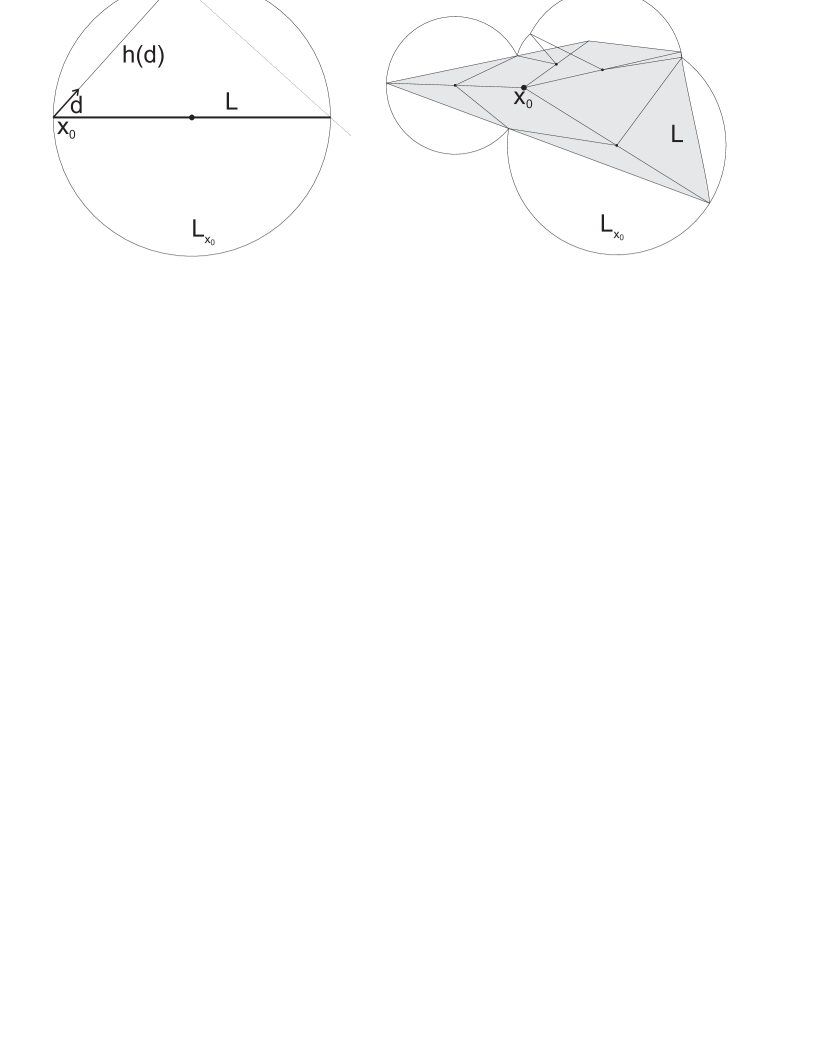
Figure 1: $L_{x_{0}}$ for a segment (left) and some polygon.

From fig. 1 we see that $L_{x_{0}}$ for a segment, where $x_{0}$ is one of its ending points, is a ball with the center in the middle of this segment.
We can threat convex set($L$) as the sum of such segments for all directions, so $L_{x_{0}}$ is the sum of all such balls (in fact we can restrict to the supporting points of $K$).
So we have rough approximations:

$$L\subset L_{x_{0}}\subset B(x_{0},R_{x_{0}})$$

$$\rho(L_{x_{0}},L)\leq R_{x_{0}}/2$$

where	$\rho(A,B):=\sup_{x\in A}\inf_{y\in B}\|x-y\|$,
	$R_{x_{0}}:=\sup_{d\in D}h_{x_{0}}(d)\ (=\inf_{r>0}\{L\subset B(x_{0},r)\})$.

If $h_{x_{0}}$ isn’t constant ($L$ is a ball) this approximation is better than with a ball.

We could go closer to $L$ this way, by checking more points, but we can use this additional checkings to came closer to the attractor - check if $x\in I^{k}(L_{x_{0}})$:

$$x\in I^{l+1}(L_{x_{0}})\Leftrightarrow\exists_{i}\ x\in A_{i}(I^{l}(L_{x_{0}}))+t_{i}\Leftrightarrow\exists_{i}\ A_{i}^{-1}(x-t_{i})\in I^{l}(L_{x_{0}})$$

If we iterate this equivalence $k$ times, we get an algorithm checking if $x\in I^{k}(L_{x_{0}})$:

function near($x$,k)
{ int i=0;
if ($x^{T}(\widehat{x-x_{0}})>h_{0}(\widehat{x-x_{0}})$) return false else
if(k=0) return true else
{ do i++ until ((i>n) or ($x\in\textrm{Im}(A_{i})$ and near($A_{i}^{-1}(x-t_{i})$,k-1)));
if(i>n) return false else return true
}
}

The condition with the image of $A_{i}$ is required for singular matrices and numerically cannot be fulfilled - we can just omit this matrices.

To evaluate the results of this algorithm, define

$$C_{k}=\rho(I^{k}(L_{x_{0}}),K)$$

$C_{0}\leq R_{x_{0}}/\sqrt{2}$ is some constant, which should be approximated from above eg numerically.

Let’s make the iteration now:

$$\inf_{y\in K}\|x-y\|=\inf_{i}\inf_{y\in K}\|x-t_{i}-A_{i}(y)\|\leq\inf_{i}\|A_{i}\|\inf_{y\in K}\|A_{i}^{-1}(x-t_{i})-y\|$$ (10)

So $C_{k}\leq C_{k-1}\max_{i}\|A_{i}\|=C_{k-1}\max_{i}c_{i}\leq C_{0}c^{k}$.

Now using (10) we can alter this algorithm: if near1($x,l$) will return true, we are sure that $x$ is nearer to $K$ than a given distance $l$:

function near1($x,l$)
{ int i=0;
if ($x^{T}(\widehat{x-x_{0}})>h_{0}(\widehat{x-x_{0}})$) return false else
if($l\geq C_{0}$) return true else
{ do i++ until ((i>n) or near1($A_{i}^{-1}(x-t_{i}),l/c_{i}$));
if(i>n) return false else return true
}
}

Analogically we can construct for example an algorithm to answer questions like if $I^{k}(L)\bigcap(I^{k}(L)+t)=\emptyset$.

5 Analytically solvable examples

In this section we will show that in some cases we can compute width function analytically.

Observation 4.

In the case $A_{1}=A_{2}=...=A_{n}(=A)$ the width function realize

$$h_{0}(d)=\|Ad\|h_{0}(\widehat{Ad})+h^{*}(d)$$ (11)

where $h^{*}(d)=\max_{i}{t_{i}^{T}d}=h_{\{t_{1},t_{2},...,t_{n}\},0}(d)$
Solution to this equation is:

$$h_{0}(d)=\sum_{i=0}^{\infty}\|A^{i}d\|h^{*}(\widehat{A^{i}d})$$ (12)

Proof: (11) is obvious from (8)
By induction over $k$, using (11):

$$h_{0}(d)=\|A^{k}d\|h_{0}(\widehat{A^{k}D})+\sum_{i=0}^{k-1}\|A^{i}d\|h^{*}(\widehat{A^{i}d})$$

$A$ is contracting, $h$ is bounded - the first term tends to 0. $\qquad\square$

Now we will show an example how to get complete set of information about the convex hull $L$ of $K$ using the width function.

Fix $X=\mathbb{R}^{2}$. We can threat $X=\mathbb{C}$ as the complex plane, multiplication by a complex number corresponds to a rotation and a scaling.
We can identify the directions space $D$ with angles: $\alpha\equiv(\cos\alpha,\sin\alpha)$.

Fix $re^{\mathbf{i}\phi}=z\in\mathbb{C}:r=|z|>1,\ 2\leq n\in\mathbb{N}$
In the rest of this section we will analyze attractor, which can represent fractional part in a complex base system[8]:

$$Kz=\sum_{i=0..n-1}\left(K+i\right)$$ (13)

Before investigating the width function, we observe that $K$ has the symmetry point:

Observation 5.

$x_{0}=\frac{1}{2}\frac{n-1}{z-1}$ is the center of symmetry of $K$.

Proof: For any point $x_{0}$, from (13) $2x_{0}-K$ satisfies:

$$z(2x_{0}-K)=2x_{0}z-\sum_{i=0..n-1}(K+i)=\sum_{k=n-1-i=0..n-1}2x_{0}z-n+1-K+k$$

Hence if $\ 2x_{0}z-n+1=2x_{0}$ then $2x_{0}=\frac{n-1}{z-1}$ and we have:

$$z(2x_{0}-K)=\sum_{i=0..n-1}(2x_{0}-K)+i$$

Because of the uniqueness: $2x_{0}-K=K$, so $\ x_{0}-K=K-x_{0}$. $\quad\quad\quad\Box$

We have $h_{x_{0}}(\alpha)\equiv h(\alpha)=h(-\alpha)=(h_{0}(\alpha)+h_{0}(-\alpha))/2$
Now $h^{*}(\alpha)+h^{*}(-\alpha)=(n-1)r^{-1}|\cos(\alpha+\phi)|$, (12) gives

$$2h(\alpha)=(n-1)\sum_{j>0}r^{-j}|\cos(\alpha+j\phi)|$$ (14)

Now assume that $\phi=\pi\frac{l}{k}\quad(l,k\in\mathbb{N})$

$$2h(\alpha)=(n-1)\sum_{j=1..k}|\cos(\alpha+j\phi)|\sum_{i\geq 0}r^{-j-ki}=\frac{n-1}{1-r^{-k}}\sum_{j=1..k}r^{-j}|\cos(\alpha+j\phi)|$$ (15)

In this case, our width function is differentiable everywhere except finite number of points. We could use (6) ($\nabla h(\widehat{\alpha})\equiv(-\sin\alpha,\cos\alpha)h^{\prime}(\alpha)$) for differentiable points of $h$ around indifferentiable, but instead we will show that this points corresponds to straight lines on the boundary of $L$ (convex hull of $K$). In fact, it will occur that $L$ is a polygon.

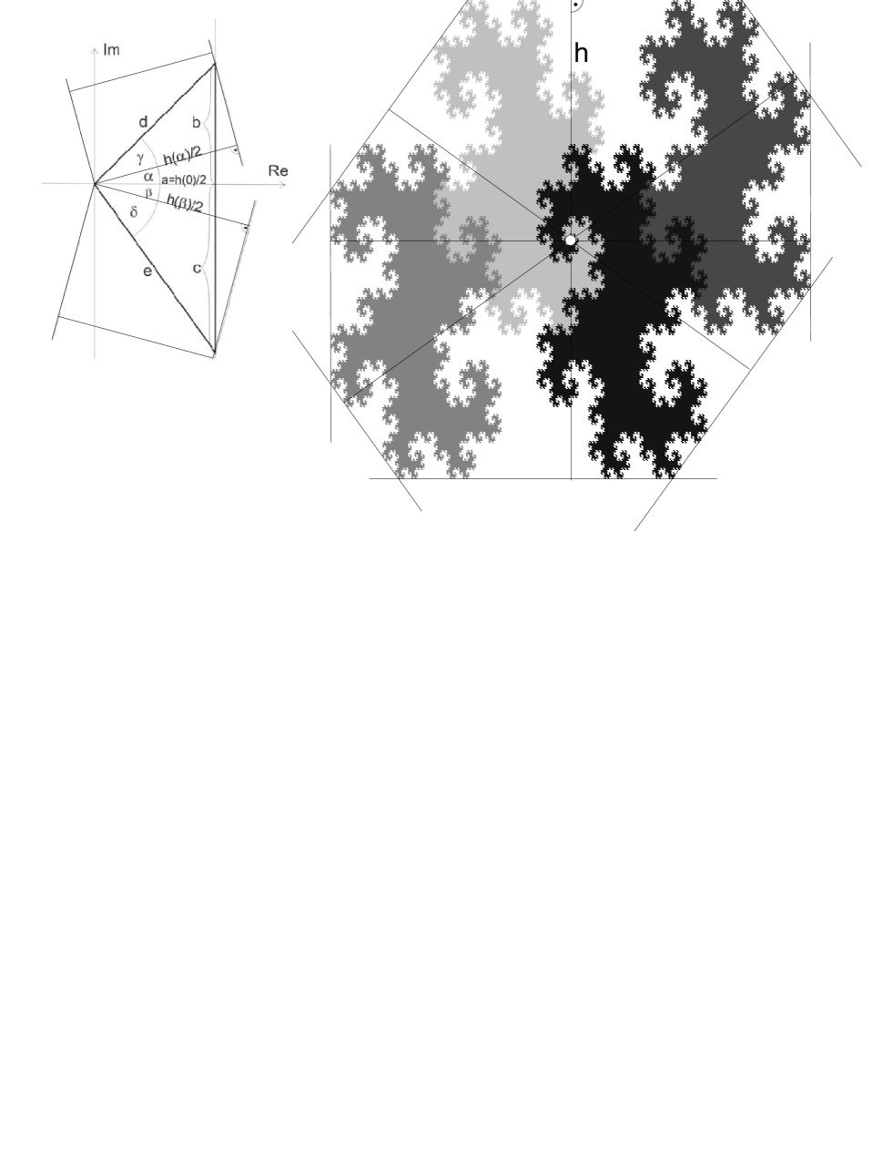
Figure 2: Analysis of the behavior of width function around a segment on the boundary of a convex set(left) and construction of the convex hull in case: $z=i+1,\ n=2$ (right).

Look at the triangle on fig. 2 - width function will have indifferentiable minimum in 0 - in a neighborhood of 0:

$$h(\alpha)=\bigg{\{}\begin{array}[]{ll}d\cos(\gamma)&0\geq\alpha<\epsilon\\ d\cos(\delta)&0>\alpha>-\epsilon\end{array}$$

$$h^{\prime}(0^{+})=d\sin(\alpha+\gamma)=b\quad,\quad h^{\prime}(0^{-})=-e\sin(\beta+\delta)=-c$$ (16)

So we see:

1. If a vertex in some direction $\gamma$ is supported by some range of directions - in that range $h(\alpha)=d\cos(\gamma-\alpha)$. Thanks to the uniqueness of $h$, implication above is equivalence.

2. In a direction in which the edge of the convex hull contains straight segment, iff the width function have local minimum and is indifferentiable.
   We can construct this segment using (16).

Now look at (15) - there is a finite number of indifferentiability points and between them function is in the form of $h(\alpha)=\sum_{i=0..k-1}a_{i}\cos(\alpha+b_{i})$. Expanding cosinus of sum, we see that it can be written in the form $h(\alpha)=a\cos(\alpha+b)$ for some $a,b\in\mathbb{R}$. So it supports on one point - common point of succeeding triangles - our convex hull is polygon.

We will construct it now - call $T(a,b,c)$ - triangle as in fig. 2
This triangles should be rotated by angles of indifferentiability $\phi_{j}:=\pi/2-j\phi\$ for $j=1..k$

$$a_{j}=h(\phi_{j})$$

$$b_{j}+c_{j}=h^{\prime}(\phi_{j}^{+})-h^{\prime}(\phi_{j}^{-})=\frac{1}{2}(n-1)\frac{r^{-j}}{1-r^{-k}}(\cos^{\prime}(\phi_{j}^{+})-\cos^{\prime}(\phi_{j}^{-}))=(n-1)\frac{r^{-j}}{1-r^{-k}}$$

$$b_{j}-c_{j}=h^{\prime}(\phi_{j}^{+})+h^{\prime}(\phi_{j}^{-})=\frac{n-1}{1-r^{-k}}\sum_{i=1..k,i\neq j}r^{-i}\frac{d}{d\alpha}|\cos(\alpha+i\phi)|_{\alpha=\phi_{j}}$$

$$L=x_{0}+\bigcup_{j=1..k}e^{i\phi_{j}}(T(a_{j},b_{j},c_{j})\cup-T(a_{j},b_{j},c_{j}))$$ (17)

Notice that if we wouldn’t gather elements with the same value of cosinus in (15) we can look on the construction above as(now $j=1..\infty$):

$$a_{j}=h(\phi_{j})$$

$$b_{j}+c_{j}=h^{\prime}(\phi_{j}^{+})-h^{\prime}(\phi_{j}^{-})=\frac{1}{2}(n-1)r^{-j}(\cos^{\prime}(\phi_{j}^{+})-\cos^{\prime}(\phi_{j}^{-}))=(n-1)r^{-j}$$

$$b_{j}-c_{j}=h^{\prime}(\phi_{j}^{+})+h^{\prime}(\phi_{j}^{-})=(n-1)\sum_{i>0,i\neq j}r^{-i}\frac{d}{d\alpha}|\cos(\alpha+i\phi)|_{\alpha=\phi_{j}}$$

$$L=x_{0}+\bigcup_{j>0}e^{i\phi_{j}}(T(a_{j},b_{j},c_{j})\cup-T(a_{j},b_{j},c_{j}))$$ (18)

In form (18) triangles from (17) are constructed from infinity many triangles with disjoint interiors.
We will use this form to construct $L$ in $\phi\notin\pi\mathbb{Q}$ case.
Take $\phi^{i}\in\pi\mathbb{Q},\ \lim_{i\to\infty}\phi^{i}=\phi$ series. We construct polygon for each $\phi^{i}$. It’s easy to check:

$$\phi_{j}^{i}\to\phi_{j}\quad\quad a_{j}^{i}\to a_{j}\quad\quad b_{j}^{i}\to b_{j}\quad\quad c_{j}^{i}\to c_{j}$$

for any $j>0$.
So (18) gives convex hull in this case.
Its boundary contains countable number of segments.

We can now find a formula for length of the boundary($B$) of $L$ and it’s area($A$):

$$B=2(n-1)\sum_{j>0}r^{-j}=2\frac{n-1}{r-1}$$

$$A = \frac{1}{2}(n-1)^{2}\sum_{i>0}r^{-i}\sum_{j>0}r^{-j}|\cos((i-j)\phi+\pi/2)|=\frac{1}{2}(n-1)^{2}|\sin(0)|(r^{-2}+r^{-4}+...)+$$

$$+ (n-1)^{2}\sum_{v:=|i-j|=1..\infty}|\sin(v\phi)|(r^{-2-v}+r^{-4-v}+...)=\frac{(n-1)^{2}}{r^{2}-1}\sum_{v>0}|\sin(v\phi)|r^{-v}$$

It’s interesting that $B$ doesn’t depends on $\phi$.

We can get an interesting trigonometric inequality from this formulas, namely we know (eg [7]) that for given length of boundary, the largest area has circle, so $A\leq B^{2}/4\pi$:

Observation 6.

$\sum_{j>0}|\sin(j\phi)|r^{-j}\leq\frac{1}{\pi}\frac{r+1}{r-1}\quad$ for any $r>1,\phi\in[0,2\pi]$.

Digression: to analyze points of indifferentiability in higher dimension - they will correspond to pyramids, which base can be analyzed by cutting space with two-dimensional planes - jumps of derivatives in different direction gives the width function for the base of pyramid. As above, we can also do it in different way - by analyzing differentiable points around indifferentiable one.

6 Conclusion

We have shown that self similarity equation can be written in terms of function describing some of its properties, like width in any direction. Other property which can be written in that way and can give some interesting results can be $f(x):=\mu(K\cap(K+x))$.
Obtained functional equation can be usually approximated numerically and used to approximate, analyze our set.
The width function can be used for example to exclude some points or to find convex hull of it and calculate some of its properties.

References

[1] H. Busemann, Convex Surfaces, Interscience Publishers, New York, 1958.
[2] J. E. Hutchinson, Fractals and self-similarity, Indiana
Univ. Math. J. 30 (1981), 713–747.
[3]J.C Hart and T.A DeFanti,Efficient anti-aliased
rendering of 3d linear fractals, SIGGRAPH ’91 Proceedings
July 1991, 91–100.
[4] J. Rice, Spatial bounding of self-affine iterated
function system attractor sets, In Graphics Interface May
1996, 107–115.
[5] A. Edalat, D.W.N. Sharp, An upper bound on the area occupied
by a fractal, Proceedings ICASSP’95. 1995. p. 2443–6
[6] Hsueh-Ting Chu and
Chaur-Chin Chen, On bounding boxes of iterated function system
attractors, Computers & Graphics 27 (2003) 407–414
[7] A. Cainchi, On relative isoperimetric
inequalities in the plane, Boll. Unione Mat. Italiana7 3-B (1989), 289-325
[8] J. Duda, Complex base numeral systems, http://arxiv.org/pdf/0712.1309