Formation, Survival, and Destruction of Vortices in Accretion Disks

Abstract

Two dimensional hydrodynamical disks are nonlinearly unstable to the formation of vortices. Once formed, these vortices essentially survive forever. What happens in three dimensions? We show with incompressible shearing box simulations that in 3D a vortex in a short box forms and survives just as in 2D. But a vortex in a tall box is unstable and is destroyed. In our simulation, the unstable vortex decays into a transient turbulent-like state that transports angular momentum outward at a nearly constant rate for hundreds of orbital times. The 3D instability that destroys vortices is a generalization of the 2D instability that forms them. We derive the conditions for these nonlinear instabilities to act by calculating the coupling between linear modes, and thereby derive the criterion for a vortex to survive in 3D as it does in 2D: the azimuthal extent of the vortex must be larger than the scale height of the accretion disk. When this criterion is violated, the vortex is unstable and decays. Because vortices are longer in azimuthal than in radial extent by a factor that is inversely proportional to their excess vorticity, a vortex with given radial extent will only survive in a 3D disk if it is sufficiently weak. This counterintuitive result explains why previous 3D simulations always yielded decaying vortices: their vortices were too strong. Weak vortices behave two-dimensionally even if their width is much less than their height because they are stabilized by rotation, and behave as Taylor-Proudman columns. We conclude that in protoplanetary disks weak vortices can trap dust and serve as the nurseries of planet formation. Decaying strong vortices might be responsible for the outwards transport of angular momentum that is required to make accretion disks accrete.

1. Introduction

Matter accretes onto a wide variety of objects, such as young stars, black holes, and white dwarfs, through accretion disks. In highly ionized disks magnetic fields are important, and they trigger turbulence via the magnetorotational instability (Balbus & Hawley, 1998). However, many disks, such as those around young stars or dwarf novae, are nearly neutral (e.g., Sano et al., 2000; Gammie & Menou, 1998). In these disks, the fluid motions are well described by hydrodynamics.

Numerical simulations of hydrodynamical disks in two-dimensions—in the plane of the disk—often produce long-lived vortices (Godon & Livio, 1999; Umurhan & Regev, 2004; Johnson & Gammie, 2005). If vortices really exist in accretion disks, they can have important consequences. First and foremost, they might generate turbulence. Since turbulence naturally transports angular momentum outwards, as is required for mass to fall inwards, it might be vortices that cause accretion disks to accrete. Second, in disks around young stars, long-lived vortices can trap solid particles and initiate the formation of planets (Barge & Sommeria, 1995).

Why do vortices naturally form in 2D simulations? Hydrodynamical disks are stable to linear perturbations. However, they are nonlinearly unstable, despite some claims to the contrary in the astrophysical literature. In two dimensions, the incompressible hydrodynamical equations of a disk are equivalent to those of a non-rotating linear shear flow (e.g., Lithwick, 2007, hereafter L07). And it has long been known that such flows are nonlinearly unstable (Gill 1965; Lerner & Knobloch 1988; L07). This nonlinear instability is just a special case of the Kelvin-Helmholtz instability. Consider a linear shear flow extending throughout the $x$-$y$ plane with velocity profile $\mbox{\boldmath$v$\unboldmath}=-qx\mbox{\boldmath$\hat{y}$\unboldmath}$, where $q>0$ is the constant shear rate, so that $-q$ is the flow’s vorticity. (In the equivalent accretion disk, the local angular speed is $\Omega=2q/3$.) This shear flow is linearly stable to infinitesimal perturbations. But if the shear profile is altered by a small amount, the alteration can itself be unstable to infinitesimal perturbations. To be specific, let the alteration be confined within a band of width $\Delta x$, and let it have vorticity $\omega=\omega(x)$ (with $|\omega|\lesssim q$), so that it induces a velocity field in excess of the linear shear with components $u_{y}\sim\omega\Delta x$ and $u_{x}=0$. Then this band is unstable to infinitesimal nonaxisymmetric (i.e. non-stream-aligned) perturbations provided roughly that

$$\left|k_{y}\right|\lesssim{1\over q}{|\omega|\over\Delta x}\ \ \Rightarrow{\rm 2D\ instability}$$ (1)

where $k_{y}$ is the wavenumber of the nonaxisymmetric perturbation. For any value of $|\omega|$ and $\Delta x$, the band is always unstable to perturbations with long enough wavelength. Remarkably, instability even occurs when $|\omega|$ is infinitesimal. Hence we may regard this as a true nonlinear instability. Balbus & Hawley (2006) assert that detailed numerical simulations have not shown evidence for nonlinear instability. The reason many simulations fail to see it is that their boxes are not long enough in the $y$-direction to encompass a small enough non-zero $|k_{y}|$.

In two dimensions, the outcome of this instability is a long-lived vortex (e.g., L07). A vortex that has been studied in detail is the Moore-Saffman vortex, which is a localized patch of spatially constant vorticity superimposed on a linear shear flow (Saffman, 1995). When $|\omega|\lesssim q$, where $\omega$ here refers to the spatially constant excess vorticity within the patch, and when the vorticity within the patch ($\omega-q$) is stronger than that of the background shear, then the patch forms a stable vortex that is elongated in $y$ relative to $x$ by the factor

$${\Delta y\over\Delta x}\sim{q\over|\omega|}\ .$$ (2)

This relation applies not only to Moore-Saffman vortices, but also to vortices whose $\omega$ is not spatially constant. It may be understood as follows. A patch with characteristic excess vorticity $\sim\omega$ and with $\Delta y\gg\Delta x$ induces a velocity field in the $x$-direction with amplitude $u_{x}\sim|\omega|\Delta x$, independent of the value of $\Delta y$ (e.g., §6 in L07). As long as $|\omega|\lesssim q$, the $y$-velocity within the vortex is predominantly due to the background shear, and is $\sim q\Delta x$. Therefore the time to cross the width of the vortex is $t_{x}\sim\Delta x/u_{x}\sim 1/|\omega|$, and the time to cross its length is $t_{y}\sim\Delta y/(q\Delta x)$. Since these times must be comparable in a vortex, equation (2) follows. Equation (2) is very similar to equation (1). The 2D instability naturally forms into a 2D vortex. Futhermore, the exponential growth rate of the instability is $\sim|\omega|$, which is comparable to the rate at which fluid circulates around the vortex.

More generally, an arbitrary axisymmetric profile of $\omega(x)$ tends to evolve into a distinctive banded structure. Roughly speaking, bands where $\omega<0$ contain vortices, and these are interspersed with bands where $\omega>0$, which contain no vortices. (Recall that we take the background vorticity to be negative; otherwise, the converse would hold.) The reason for this is that only regions that have $\omega<0$ can be unstable, as may be inferred either from the integral criterion for instability given in footnote 2, or from Fjørtoft’s theorem. For more detail on vortex dynamics in shear flows, see the review by Marcus (1993).

What happens in three dimensions? To date, numerical simulations of vortices in 3D disks have been reported in two papers. Barranco & Marcus (2005) initialized their simulation with a Moore-Saffman vortex, and solved the anelastic equations in a stratified disk. They found that this vortex decayed. As it decayed, new vortices were formed in the disk’s atmosphere, two scale heights above the midplane. The new vortices survived for the duration of the simulation. Shen et al. (2006) performed both 2D and 3D simulations of the compressible hydrodynamical equations in an unstratified disk, initialized with large random fluctuations. They found that whereas the 2D simulations produced long-lived vortices, in three dimensions vortices rapidly decayed.

Intuitively, it seems clear that a vortex in a very thin disk will behave as it does in 2D. And from the 3D simulations described above it may be inferred that placing this vortex in a very thick disk will induce its decay. Our main goal in this paper is to understand these two behaviors, and the transition between them. A crude explanation of our final result is that vortices decay when the 2D vortex motion couples resonantly to 3D modes, i.e., to modes that have vertical wavenumber $k_{z}\neq 0$. As described above, a vortex with excess vorticity $|\omega|$ has circulation frequency $\sim|\omega|$, and $k_{y}/k_{x}\sim|\omega|/q$, where $k_{x}$ and $k_{y}$ are its “typical” wavenumbers. Furthermore, it is well-known that the frequency of axisymmetric ($k_{y}=0$) inertial waves is $\Omega k_{z}/\sqrt{k_{x}^{2}+k_{z}^{2}}$ (see eq. [43]). Equating the two frequencies, and taking the $k_{x}$ of the 3D mode to be comparable to the $k_{x}$ of the vortex, as well as setting $q=3\Omega/2$ for a Keplerian disk, we find

$$k_{z}\sim k_{y}$$ (3)

as the condition for resonance. Therefore a vortex with length $\Delta y$ will survive in a box with height $\Delta z\lesssim\Delta y$, because in such a box all 3D modes have too high a frequency to couple with the vortex, i.e., all nonzero $k_{z}$ exceed the characteristic $k_{y}\sim 1/\Delta y$. But when $\Delta z\gtrsim\Delta y$, there exist $k_{z}$ in the box that satisfy the resonance condition (3), leading to the vortex’s destruction. This conclusion suggests that vortices live indefinitely in disks with scale height less than their length ($h\lesssim\Delta y$) because in such disks all 3D modes have too high a frequency for resonant coupling. This conclusion is also consistent with the simulations of Barranco & Marcus (2005) and Shen et al. (2006). Both of these works initialized their simulations with strong excess vorticity $|\omega|\sim q$, corresponding to nearly circular vortices. Both had vertical domains that were comparable to the vortices’ width. Therefore both saw that their vortices decayed. Had they initialized their simulations with smaller $|\omega|$, and increased the box length $L_{y}$ to encompass the resulting elongated vortices, both would have found long-lived 3D vortices. Barranco & Marcus’s discovery of long-lived vortices in the disk’s atmosphere is simple to understand because the local scale height is reduced in inverse proportion to the height above the midplane. Therefore higher up in the atmosphere the dynamics becomes more two-dimensional, and a given vortex is better able to survive the higher it is.

1.1. Organization of the Paper

In §2 we introduce the equations of motion, and in §3 we present two pseudospectral simulations. One illustrates the formation and survival of a vortex in a short box, and the other illustrates the destruction of a vortex in a tall box.

In §§4-5 we develop a theory explaining this behavior. The reader who is satisfied by the qualitative description leading to equation (3) may skip those two sections. The theory that we develop is indirectly related to the transient amplification scenario for the generation of turbulence. Even though hydrodynamical disks are linearly stable, linear perturbations can be transiently amplified before they decay, often by a large factor. It has been proposed that sufficiently amplified modes might couple nonlinearly, leading to turbulence (e.g., Chagelishvili et al., 2003; Yecko, 2004; Afshordi et al., 2005). However, to make this proposal more concrete, one must work out how modes couple nonlinearly. In L07, we did that in two dimensions. We showed that the 2D nonlinear instability of equation (1) is a consequence of the coupling of an axisymmetric mode with a transiently amplified mode, which may be called a “swinging mode” because its phasefronts are swung around by the background shear. In §5 we show that the 3D instability responsible for the destruction of vortices is a generalization of this 2D instability. It may be understood by examining the coupling of a 3D swinging mode with an axisymmetric one. 3D modes become increasingly unstable as $|k_{z}|$ decreases, and in the limit that $k_{z}\rightarrow 0$, the 3D instability matches smoothly onto the 2D one. Thicker disks are more prone to 3D instability because they encompass smaller $|k_{z}|$.

2. Equations of Motion

We solve the “shearing box” equations, which approximate the dynamics in an accretion disk on lengthscales much smaller than the distance to the disk’s center. We assume incompressibility, which is a good approximation when relative motions are subsonic. We also neglect vertical gravity, and hence stratification and buoyancy, which is an oversimplification. To fully understand vortices in astrophysical disks, one must consider the effects of vertical gravity as well as of shear and rotation. In this paper, we consider only two pieces of this puzzle—shear and rotation. Adding the third piece—vertical gravity—is a topic that we leave for future investigations. See also the Conclusions for some speculations.

An unperturbed Keplerian disk has angular velocity profile $\Omega(r)\propto r^{-3/2}$. In a reference frame rotating at constant angular speed $\Omega_{0}\equiv\Omega(r_{0})$, where $r_{0}$ is a fiducial radius, the incompressible shearing box equations of motion read

$${\partial_{t}{\mbox{\boldmath$v$\unboldmath}}}+{\mbox{\boldmath$v\cdot\nabla v$\unboldmath}} = -2\Omega_{0}{\mbox{\boldmath$\hat{z}$\unboldmath}}{\mbox{\boldmath$\times v$\unboldmath}}+2q\Omega_{0}x{\mbox{\boldmath$\hat{x}$\unboldmath}}-{\mbox{\boldmath$\nabla$\unboldmath}}P/\rho\ \ ,$$ (4)

$$\nabla\cdot v = 0$$ (5)

adopting Cartesian coordinates $x,y,z$, which are related to the disk’s cylindrical $r,\theta$ via $x\equiv r-r_{0}$ and $y\equiv r_{0}(\theta-\Omega_{0}t)$; $\hat{x}$ and $\hat{z}$ are unit vectors, and

$$q\equiv-{d\Omega\over d\ln r}\Big{|}_{r_{0}}={3\over 2}\Omega_{0}\ ,$$ (6)

We retain $q$ and $\Omega_{0}$ as independent parameters because they parameterize different effects: shear and rotation, respectively. The first term on the right-hand side of equation (4) is the Coriolis force, and the second is what remains after adding centrifugal and gravitational forces. Decomposing the velocity into

$$\mbox{\boldmath$v$\unboldmath}=-qx\mbox{\boldmath$\hat{y}$\unboldmath}+\mbox{\boldmath$u$\unboldmath}\ ,$$ (7)

where the first term is the shear flow of the unperturbed disk, yields

$$\left({\partial_{t}}-qx{\partial_{y}}\right){\mbox{\boldmath$u$\unboldmath}}+{\mbox{\boldmath$u\cdot\nabla u$\unboldmath}} = qu_{x}\mbox{\boldmath$\hat{y}$\unboldmath}-2\Omega{\mbox{\boldmath$\hat{z}$\unboldmath}}{\mbox{\boldmath$\times u$\unboldmath}}-\mbox{\boldmath$\nabla$\unboldmath}P/\rho$$ (8)

$$\nabla\cdot u = 0\ ,$$ (9)

dropping the subscript from $\Omega_{0}$, as we shall do in the remainder of this paper. An unperturbed disk has $\mbox{\boldmath$u$\unboldmath}=0$.

In addition to the above “velocity-pressure” formulation, an alternative “velocity-vorticity” formulation will prove convenient. It is given by the curl of equation (8),

$$(\partial_{t}-qx\partial_{y})\mbox{\boldmath$\omega$\unboldmath}=-q\mbox{\boldmath$\hat{y}$\unboldmath}\omega_{x}+(2\Omega-q)\partial_{z}\mbox{\boldmath$u$\unboldmath}+\mbox{\boldmath$\nabla\times$\unboldmath}(\mbox{\boldmath$u\times\omega$\unboldmath})$$ (10)

where

$$\mbox{\boldmath$\omega$\unboldmath}\equiv\mbox{\boldmath$\nabla\times u$\unboldmath}$$ (11)

is the vorticity of $u$. Equation (10), together with the inverse of equation (11)

$$\mbox{\boldmath$u$\unboldmath}=-\nabla^{-2}\mbox{\boldmath$\nabla\times\omega$\unboldmath}\ ,$$ (12)

form a complete set.

Equation (10) implies that the total vorticity field is frozen into the fluid, because it is equivalent to

$$\partial_{t}\mbox{\boldmath$\omega$\unboldmath}_{\rm tot}=\mbox{\boldmath$\nabla\times$\unboldmath}(\mbox{\boldmath$v\times\omega$\unboldmath}_{\rm tot})\ ,$$ (13)

where

$${\mbox{\boldmath$\omega$\unboldmath}}_{\rm tot}\equiv(2\Omega-q)\mbox{\boldmath$\hat{z}$\unboldmath}+\mbox{\boldmath$\omega$\unboldmath}\$$ (14)

is the total vorticity; note that $-q\mbox{\boldmath$\hat{z}$\unboldmath}$ is the vorticity of the unperturbed shear flow in the rotating frame, and hence $(2\Omega-q)\mbox{\boldmath$\hat{z}$\unboldmath}$ is the unperturbed vorticity in the non-rotating frame. The vorticity-velocity picture is similar to MHD, where it is the magnetic field that is frozen-in because it satisfies equation (13) in place of $\mbox{\boldmath$\omega$\unboldmath}_{\rm tot}$. However, in MHD the velocity field has its own dynamical equation, whereas in incompressible hydrodynamics it is determined directly from the vorticity field via equation (12).

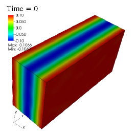
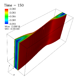
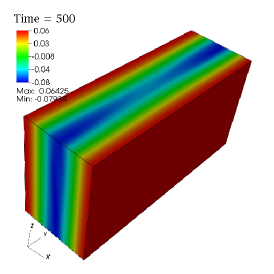
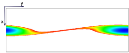
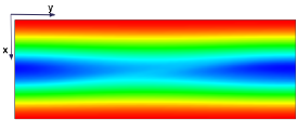
Figure 1.— Vortex Formation and Survival in a Short Box: Color depicts $\omega_{z}$. The initial state is unstable to vertically symmetric ($k_{z}=0$) perturbations, and forms into a vortex. But it is stable to 3D ($k_{z}\neq 0$) perturbations, and the evolution remains two-dimensional. The bottom panels show horizontal slices through the boxes in the upper panels, midway through the boxes. At time=150, the vortex has already formed. Only fluid with $\omega_{z}<-0.08$ is shown in the middle panels to highlight the vortex, and to illustrate that surfaces of constant $\omega_{z}$ remain purely vertical. At time=500, the vortex still survives. Its amplitude is slowly decaying by viscosity, which acts on timescale=1130. We set $\Omega=1$ and $q=3/2$. The number of modes in the simulation is $n_{x}\times n_{y}\times n_{z}=64\times 64\times 32$, and the size of the simulation box is $(L_{x},L_{y},L_{z})=({1\over 15},1,{1\over 2})$. In this figure, $L_{z}$ is to scale relative to $L_{y}$, but $L_{x}$ has been expanded by a factor of 5 for clarity.

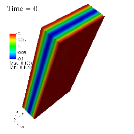
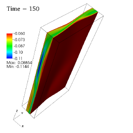
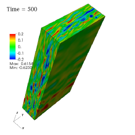
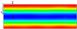
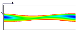
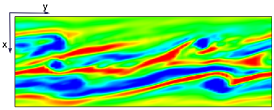
Figure 2.— Vortex Destruction in a Tall Box: The setup is identical to the short-box simulation of Figure 1, except that the height $L_{z}$ has been increased by a factor of 4, so that it now exceeds $L_{y}$. The resulting evolution is dramatically different. The initial state is now unstable not only to 2D perturbations, but to 3D ones as well. In the middle panels, surfaces of constant $\omega_{z}$ are warped, and the evolution is no longer vertically symmetric. In the right panels, the flow looks turbulent.

Figure 3.— Energy in the Short Box: The three contributions to the energy budget, $E_{u^{2}}$, $\Delta E_{\rm shear}$, and $\Delta E_{\rm visc}$, are defined in equations (20)-(22). $E_{u^{2}}$ initially decays, and then rises to a peak near $t\sim 200$ as nonaxisymmetric perturbations turn the axisymmetric mode into a vortex. Subsequently, the vortex decays due to viscosity. The spikiness of the evolution is due to the boundary conditions, as explained in the text. Also shown in the bottom panel is the error due to numerical effects, $\Delta E_{\rm error}$ (eq. [24]). It is unlabelled because it is mostly obscured by $\Delta E_{\rm shear}$. But it is nearly equal to zero everywhere, showing that the code accurately tracks the components of the energy budget.

Figure 4.— Energy in the Tall Box: The initial evolution is almost the same as that seen in the short box (Fig. 3). But 3D perturbations are unstable and force the destruction of the vortex. In the time interval $300\lesssim t\lesssim 600$, while the initial axisymmetric disturbance decays in a turbulent-like state, the value of $E_{u^{2}}$ is significantly larger than its initial value, and $\Delta E_{\rm shear}$ rises nearly linearly in time, corresponding to nearly constant outwards transport of angular momentum in a disk. The contribution of numerical errors to the time-integrated energy budget, $\Delta E_{\rm error}$ (eq. [24]), remains small throughout.

3. Two Pseudospectral Simulations

The pseudospectral code is described in detail in the Appendix of L07. It solves the velocity-pressure equations of motion with an explicit viscous term

$$\nu\nabla^{2}{\mbox{\boldmath$u$\unboldmath}}$$ (15)

added to equation (8). (In L07, we did not include this term because we only considered inviscid flows.) The equations are solved in Fourier-space by decomposing fields into spatial Fourier modes whose wavevectors are advected by the background flow $-qx\mbox{\boldmath$\hat{y}$\unboldmath}$. As a result, the boundary conditions are periodic in the $y$ and $z$ dimension, and “shearing periodic” in $x$. Most of our techniques are standard (e.g., Maron & Goldreich, 2001; Rogallo, 1981; Barranco & Marcus, 2006). One exception is our method for remapping highly trailing wavevectors into highly leading ones, which is both simpler and more accurate than the usual method. In addition, our remapping does not introduce power into leading modes, because a mode’s amplitude has always been set to zero before the remap. The code was extensively tested on 2D flows in L07. A number of rather stringent 3D tests are performed in this paper. We shall show that the code correctly reproduces the linear evolution of 3D modes (§4), as well as the nonlinear coupling between them (§5). We also show in the present section that it tracks the various contributions to the energy budget, and that the sum of the contributions vanishes to high accuracy.

Figures 1-4 show results from two pseudospectral simulations. One simulation illustrates the formation and survival of a vortex, and the other illustrates vortex destruction. In the first (the “short box”), the number of Fourier modes used is $n_{x}\times n_{y}\times n_{z}=64\times 64\times 32$, and the simulation box has dimensions $L_{x}={1\over 15}$, $L_{y}=1$, and $L_{z}={1\over 2}$. In the second (the “tall box”), the setup is identical, except that it has $L_{z}=2$ instead of $1/2$. Both simulations are initialized by setting

$$\omega_{z}\Big{|}_{t=0}=-0.1\cos\left({2\pi\over L_{x}}x\right)\ .$$ (16)

In addition, small perturbations are added to long-wavelength modes. Specifically, labelling the wavevectors as

$$(k_{x},k_{y},k_{z})=2\pi\left({j_{x}\over L_{x}},{j_{y}\over L_{y}},{j_{z}\over L_{z}}\right)\ ,$$ (17)

with integers $(j_{x},j_{y},j_{z})$, we select all modes that satisfy $|j_{x}|\leq 3$, $|j_{y}|\leq 3$, and $|j_{z}|\leq 3$, and set the Fourier amplitude of their $\omega_{z}$ to $10^{-4}e^{i\phi}$, where $\phi$ is a random phase. But we exclude the $(j_{x},j_{y},j_{z})=(0,0,0)$ mode, as well as $(j_{x},j_{y},j_{z})=(\pm 1,0,0)$, which is given by equation (16). Finally, we set $\Omega=1$, $q=3/2$, $\nu=10^{-7}$, and integration timestep $dt=1/30$.

With our chosen initial conditions, the mode given by equation (16) is nonlinearly unstable to vertically symmetric ($k_{z}=0$) perturbations, and hence it tends to wrap up into a vortex. From the approximate criterion for instability (eq. [1]), we see that to illustrate the wrapping up into a vortex of a mode with a small amplitude, one must make the simulation box elongated in the $y$-direction relative to the $x$-scale of the mode in equation (16).

In the short box (Fig. 1), the evolution proceeds just as it would in two dimensions. The initial mode indeed wraps up into a vortex, and the evolution remains vertically symmetric throughout. Once formed, the vortex can live for ever in the absence of viscosity. But in our simulation, there is a slow viscous decay. The timescale for viscous decay across the width of the vortex is $\sim 1/\nu k_{x}^{2}=1130$, taking $k_{x}=2\pi/L_{x}$.

In the tall box (Fig. 2), the evolution is dramatically different. In this case, the initial state is unstable not only to 2D perturbations, but to 3D $(k_{z}\neq 0)$ ones as well. In the middle panel of that figure, we see that instead of forming a vertically symmetric vortex as in the short box, surfaces of constant $\omega_{z}$ are warped. By the third panel, the flow looks turbulent.

Figures 3-4 shows the evolution of the energy in these simulations. Projecting $u$ onto the Navier-Stokes equation (eq. [8] with viscosity included), and spatially averaging, we arrive at the energy equation

$${d\over dt}{\left\langle u^{2}\right\rangle\over 2}=q\langle u_{x}u_{y}\rangle+\nu\langle{\mbox{\boldmath$u$\unboldmath}\cdot}\nabla^{2}\mbox{\boldmath$u$\unboldmath}\rangle\ ,$$ (18)

after applying the shearing-box boundary conditions, where angled brackets denote a spatial average. The time integral of this equation is

$$E_{u^{2}}-E_{u^{2}}|_{t=0}=\Delta E_{\rm shear}+\Delta E_{\rm visc}\ ,$$ (19)

where

$$E_{u^{2}} \equiv {\left\langle u^{2}\right\rangle\over 2}$$ (20)

$$\Delta E_{\rm shear} \equiv q\int_{0}^{t}\langle u_{x}u_{y}\rangle dt^{\prime}$$ (21)

$$\Delta E_{\rm visc} \equiv \nu\int_{0}^{t}\langle{\mbox{\boldmath$u$\unboldmath}\cdot}\nabla^{2}\mbox{\boldmath$u$\unboldmath}\rangle dt^{\prime}\ .$$ (22)

The pseudospectral code records each of these terms, and Figure 3 shows the result in the short box simulation. At very early times, $E_{u^{2}}$ decays from its initial value due to viscosity. At the same time, the small vertically symmetric perturbations are growing exponentially, and they start to give order unity perturbations by $t\sim 150$, by which time a vortex has been formed (Fig. 1). As time evolves, $E_{u^{2}}$ gradually decays due to viscosity on the viscous timescale $=1130$. The evolution is very spiky. We defer a discussion of this spikiness to the end of this section.

Figure 4 shows the result in the tall box. The early evolution of $E_{u^{2}}$ is similar to that seen in the short box. Both start with the same $E_{u^{2}}$, and an initial period of viscous decay is interrupted by exponentially growing perturbations. But in the tall box, not only are vertically symmetric modes growing, but modes with $k_{z}\neq 0$ are growing as well. By $t\sim 150$, there is a distorted vortex that subsequently decays into a turbulent-like state. The energy $E_{u^{2}}$ rises to a value significantly larger than its initial one, and it continues to rise until $t\sim 600$, when it starts to decay. Throughout the time interval $300\lesssim t\lesssim 600$, $\Delta E_{\rm shear}$ rises nearly linearly in time, showing that $\langle u_{x}u_{y}\rangle$ is positive and nearly constant.

It is intriguing that $\langle u_{x}u_{y}\rangle$ is positive for hundreds of orbits, because it suggests that decaying vortices might transport angular momentum outwards in disks and hence drive accretion. Understanding the level of the turbulence, its lifetime, and its nature are topics for future work. Here we merely address the sign of $\langle u_{x}u_{y}\rangle$. The quantity $\langle u_{x}u_{y}\rangle$ is the flux of $y$-momentum in the $+x$-direction (per unit mass and spatially averaged). It corresponds to the flux of angular momentum in a disk. A positive $\langle u_{x}u_{y}\rangle$ implies an outwards flux of angular momentum, as is required to drive matter inwards in an accretion disk. (Even though the shearing box cannot distinguish inwards from outwards, the sign of the angular momentum within a box depends on which side of the shearing box one calls inwards. Therefore, outwards transport of (positive) angular momentum is well-defined in a shearing box.) In the shearing box, any force that tends to diminish the background shear flow $-qx\mbox{\boldmath$\hat{y}$\unboldmath}$ necessarily transports $y$-momentum in the $+x$-direction. Hence the fact that $\langle u_{x}u_{y}\rangle>0$ in Figure 4 shows that the turbulence exerts forces that resist the background shear, as one might expect on physical grounds. One can also understand why $\langle u_{x}u_{y}\rangle>0$ from energy considerations. Since $\Delta E_{\rm visc}<0$, as may be seen explicitly by an integration by parts, i.e. $\langle\mbox{\boldmath$u\cdot$\unboldmath}\nabla^{2}\mbox{\boldmath$u$\unboldmath}\rangle=-\sum_{i,j}\langle(\partial_{j}u_{i})^{2}\rangle$, equation (19) may be rearranged to read

$$\Delta E_{\rm shear}=\left|\Delta E_{\rm visc}\right|+E_{u^{2}}-E_{u^{2}}|_{t=0}\ .$$ (23)

If the turbulence reaches a steady state—as it approximately does in Figure 4 during the time interval $300\lesssim t\lesssim 600$—then the last two terms in the above equation are nearly constant, whereas $\left|\Delta E_{\rm visc}\right|$ increases linearly with time. Hence $\Delta E_{\rm shear}$ must also increase. The fact that energy dissipation implies outwards transport of angular momentum is a general property of accretion disks (e.g., Lynden-Bell & Pringle, 1974). Since turbulence always dissipates energy, it must also transport angular momentum outwards. However, this argument can be violated if an external energy source drives the turbulence, in which case one would have to add this energy to the left-hand side of equation (23). For example, the simulations of Stone & Balbus (1996) show that convective disks can transport angular momentum inwards when an externally imposed heat source drives the convection.

Also shown in the bottom panels of Figures 3-4 is the integrated energy error

$$\Delta E_{\rm error}\equiv\Delta E_{\rm shear}+\Delta E_{\rm visc}+E_{u^{2}}|_{t=0}-E_{u^{2}}$$ (24)

due to numerical effects, which is seen to be small. (In Figure 3, $\Delta E_{\rm error}$ is not labelled because the curve is mostly obscured by $\Delta E_{\rm shear}$; it can be seen near $t\sim 200$, and is everywhere very nearly equal to zero.) The fact that $\Delta E_{\rm error}$ nearly vanishes throughout the simulations is not guaranteed by the pseudospectral algorithm. Rather, we have chosen $\nu$ to be large enough that the algorithm introduces negligible error into the energy budget. To be more precise, at each timestep in the pseudospectral code, modes that have $|j_{x}|>n_{x}/3$ or $|j_{y}|>n_{y}/3$ or $|j_{z}|>n_{z}/3$, where $j_{x,y,z}$ are defined via equation (17), have their amplitudes set to zero (“dealiased”). This introduces an error that is analogous to grid error in grid-based codes. By choosing $\nu$ to be sufficiently large, it is the explicit viscosity that forces modes with large $k$ to have small amplitudes, in which case the dealiasing procedure has little effect on the dynamics. Increasing the resolution $n_{x}\times n_{y}\times n_{z}$ would allow a smaller $\nu$ to be chosen—implying a larger effective Reynolds number—while keeping the energy error small.

The curves of $E_{u^{2}}$ show sharp narrow spikes every time interval $\Delta t=10$, with width $\sim 1$. Similar spikes have been seen in other simulations (Umurhan & Regev, 2004; Shen et al., 2006), but they are stronger and narrower in our simulations because our simulation box is elongated. These spikes are due to the shearing-periodic boundary conditions. It is perhaps simplest to understand them by following the evolution in $k$-space, as we shall do in §5 (see also L07). But for now, we explain their origin in real-space. By the nature of shearing-periodic boundary conditions, associated with the simulation box centered at $x=0$ are “imaginary boxes” centered at $x=jL_{x}$ with integer $j=\pm 1,\pm 2,\cdots$. These imaginary boxes completely tile the $x-y$ plane, and each contains a virtual copy of the conditions inside the simulation box. The boxes move relative to the simulation box in the $y$-direction, with the speed of the mean shear at the center of each box, $-qjL_{x}$. Therefore, in the time interval $\Delta t=L_{y}/(qL_{x})=10$, all the boxes line up. When this happens, the velocity field $u$ that is induced by the vorticity within all the boxes (via eq. [12]) becomes large, because all the boxes reinforce each other, and therefore $E_{u^{2}}$ exhibits a spike. Even though the shearing-periodic boundary conditions that we use are somewhat artificial, we are confident that using more realistic open boundary conditions would not affect the main results of this paper—and particularly not the stability of axisymmetric modes to 3D perturbations. In L07, where we considered 2D dynamics, we investigated both open and shearing-periodic boundary conditions, and showed explicitly that both give similar results. We also feel that the boundary conditions likely do not affect the level and persistence of the “turbulence” seen in Figure 4. However, this is less certain. Future investigations should more carefully address the role of boundary conditions.

4. Linear Evolution

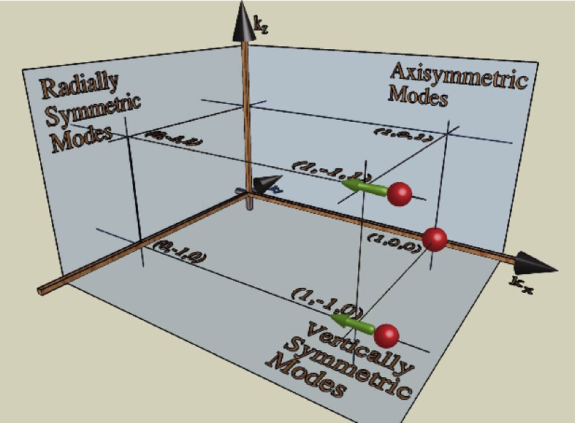
Figure 5.— Evolution of Wavevectors: Modes have constant $k_{y}$ and $k_{z}$, and $k_{x}=qtk_{y}+$const. The three spheres depict modes that play important roles in nonlinear instability. The mode at $(1,0,0)$ does not move in $k$-space. The other two modes are swinging modes that are depicted in the leading phase of their swing. They will become trailing after crossing through the radially symmetric plane. The mode crossing through $(1,-1,0)$ is responsible for 2D instability that forms vortices. The one crossing through $(1,-1,1)$ is responsible for 3D instability that destroys vortices.

In the remainder of this paper, we develop a theory explaining the stability of vortices seen in the above numerical simulations. We first consider the linear evolution of individual modes, and then proceed to show how nonlinear coupling between linear modes can explain vortex stability.

The linear evolution has been considered previously (Afshordi et al., 2005; Johnson & Gammie, 2005; Balbus & Hawley, 2006). Only two aspects of our treatment are new. First, we give the solution in terms of variables that allow the simple reconstruction of the full vectors $\omega$ and $u$. And second, we give the analytic expression for matching a leading mode onto a trailing mode that is valid for all $k_{y}$ and $k_{z}$,

The linearized equation of motion is (eq. [10])

$$(\partial_{t}-qx\partial_{y})\mbox{\boldmath$\omega$\unboldmath}=-q\mbox{\boldmath$\hat{y}$\unboldmath}\omega_{x}+(2\Omega-q)\partial_{z}\mbox{\boldmath$u$\unboldmath}\ .$$ (25)

A single mode may be written as

$$\mbox{\boldmath$\omega$\unboldmath}(\mbox{\boldmath$x$\unboldmath},t)=\mbox{\boldmath$\hat{\omega}$\unboldmath}(\mbox{\boldmath$k_{0}$\unboldmath},t)e^{i\left[{\mbox{\boldmath$k$\unboldmath}}\left({\mbox{\boldmath$k_{0}$\unboldmath}},t\right)\right]{\mbox{\boldmath$\cdot$\unboldmath}}\mbox{\boldmath$x$\unboldmath}}\ ,$$ (26)

where $k_{0}$ is a constant vector that denotes the wavevector at time $t=0$, and the wavevector $\mbox{\boldmath$k$\unboldmath}=\mbox{\boldmath$k$\unboldmath}(\mbox{\boldmath$k_{0}$\unboldmath},t)$ has components

$$k_{y} = k_{0y}={\rm const}$$ (27)

$$k_{z} = k_{0z}={\rm const}$$ (28)

$$k_{x} = {k_{0x}}+qtk_{y}\neq{\rm const}\ ,$$ (29)

so that upon insertion into equation (25), the time-derivative of the exponential cancels the term $-qx\partial_{y}{\mbox{\boldmath$\omega$\unboldmath}}$. The velocity field induced by such a mode is (eq. [12])

$$\mbox{\boldmath$u$\unboldmath}(\mbox{\boldmath$x$\unboldmath},t)=\mbox{\boldmath$\hat{u}$\unboldmath}(\mbox{\boldmath$k_{0}$\unboldmath},t)e^{i\mbox{\boldmath$k$\unboldmath}\left[\left({\mbox{\boldmath$k_{0}$\unboldmath}},t\right)\right]{\mbox{\boldmath$\cdot$\unboldmath}}\mbox{\boldmath$x$\unboldmath}}$$ (30)

where

$$\mbox{\boldmath$\hat{u}$\unboldmath}=i{\mbox{\boldmath$k\times\hat{\omega}$\unboldmath}\over k^{2}}$$ (31)

Figure 5 sketches the evolution of wavevectors. Axisymmetric modes ($k_{y}=0$) do not move in $k$-space, as depicted by the sphere at $(1,0,0)$ in Figure 5. “Swinging modes” have $k_{y}\neq 0$, and their $k_{x}$ is time-dependent. Their fronts of constant phase are advected by the background shear. Swinging modes with $k_{x}/k_{y}<0$, as depicted by the two spheres near $(1,-1,0)$ and $(1,-1,1)$ in Figure 5, have phasefronts tilted into the background shear, i.e., they are leading modes. As time evolves, the shear first swings their $k_{x}$ through $k_{x}=0$, at which point their phasefronts are radially symmetric. Subsequently, they become trailing modes ($k_{x}/k_{y}>0$), and approach alignment with the azimuthal direction ($k_{x}/k_{y}\rightarrow\infty$).

We turn now to the evolution of the Fourier amplitudes. In the remainder of this paper we drop the hats

$$\mbox{\boldmath$\hat{\omega}$\unboldmath}\rightarrow\mbox{\boldmath$\omega$\unboldmath}\ ,\ \ \mbox{\boldmath$\hat{u}$\unboldmath}\rightarrow\mbox{\boldmath$u$\unboldmath}\ .$$ (32)

To distinguish real-space fields, we shall explicitly write their spatial dependence, e.g. $\mbox{\boldmath$\omega$\unboldmath}(\mbox{\boldmath$x$\unboldmath})$.

Because $\mbox{\boldmath$\omega$\unboldmath}(\mbox{\boldmath$x$\unboldmath})$ is divergenceless, ${\omega}$ only has two degrees of freedom, which we select to be ${\omega}_{x}$ and

$${\omega}_{yz}\equiv{\mbox{\boldmath$\hat{x}\cdot$\unboldmath}\left({{\mbox{\boldmath$k\times{\omega}$\unboldmath}}}\right)\over k_{yz}}=\left\{\begin{array}[]{r@{\quad,\quad}l}-{\omega}_{y}&{\rm if\ }k_{y}=0\\ {\omega}_{z}&{\rm if\ }k_{z}=0\end{array}\right.$$ (35)

where

$$k_{yz}\equiv\sqrt{k_{y}^{2}+k_{z}^{2}}$$ (36)

Our variable $\omega_{yz}$ is proportional to the variable $U$ of Balbus & Hawley (2006). Adopting $\omega_{x}$ as the second degree of freedom enables the full vectors to be reconstructed as

$${\omega} = -{\omega}_{x}{\mbox{\boldmath$k\times$\unboldmath}(\mbox{\boldmath$k\times\hat{x}$\unboldmath})\over k_{yz}^{2}}-{{\omega}_{yz}}{\mbox{\boldmath$k\times\hat{x}$\unboldmath}\over k_{yz}}$$ (37)

$${u} = -i\omega_{yz}{\mbox{\boldmath$k\times$\unboldmath}(\mbox{\boldmath$k\times\hat{x}$\unboldmath})\over k^{2}k_{yz}}+i\omega_{x}{\mbox{\boldmath$k\times\hat{x}$\unboldmath}\over k_{yz}^{2}}$$ (38)

The linearized equation (25) is expressed in terms of these degrees of freedom as

$${k_{yz}\over qk_{y}}{d\over dt}\left(\begin{array}[]{c}{\omega}_{x}\\ {\omega}_{yz}\end{array}\right)=\beta{\Omega\over\kappa}\left(\begin{array}[]{cc}0&-{1\over 2}{\kappa^{2}\over\Omega^{2}}{1\over 1+\tau^{2}}\\ 2&0\end{array}\right)\left(\begin{array}[]{c}{\omega}_{x}\\ {\omega}_{yz}\end{array}\right)\ ,$$ (39)

after introducing the epicyclic frequency,

$$\kappa\equiv\sqrt{2\Omega(2\Omega-q)}\ ,$$ (40)

with $\kappa=\Omega$ in a Keplerian disks, and

$$\tau \equiv {k_{x}\over k_{yz}}$$ (41)

$$\beta \equiv {\kappa\over q}{k_{z}\over k_{y}}\ .$$ (42)

As long as $k_{y}\neq 0$, $\tau$ varies in time through its dependence on $k_{x}=k_{0x}+qtk_{y}$.

For axisymmetric modes ($k_{y}=0$), $\tau$ is constant and

$${d^{2}\over dt^{2}}\omega_{yz}+\kappa^{2}{k_{z}^{2}\over k_{x}^{2}+k_{z}^{2}}\omega_{yz}=0\ ,$$ (43)

the solution of which is sinusoidal with frequency $\kappa k_{z}/\sqrt{k_{x}^{2}+k_{z}^{2}}$. Axisymmetric modes with phasefronts aligned with the plane of the disk ($k_{x}=k_{y}=0$) have in-plane fluid velocities, and they oscillate at the epicyclic frequency of a free test particle, $\kappa$. But axisymmetric modes with tilted phasefronts have slower frequencies, because fluid pressure causes deviations from free epicycles. In the limit of vertical axisymmetric phasefronts ($k_{z}=k_{y}=0$), the effects of rotation disappear entirely, and this zero-frequency mode merely alters the mean shear flow’s velocity profile.

For swinging modes ($k_{y}\neq 0$), it is convenient to employ $\tau$ as the time variable. Since

$${k_{yz}\over qk_{y}}{d\over dt}={d\over d\tau}\ ,$$ (44)

we have

$${d^{2}\over d\tau^{2}}\omega_{yz}+{\beta^{2}\over 1+\tau^{2}}\omega_{yz}=0\ .$$ (45)

(Balbus & Hawley, 2006). Figure 6 plots numerical solutions of this equation, and shows that it matches the output from the pseudospectral code, as well as the analytic theory described below. Given $\omega_{yz}$, it is trivial to construct $\omega$ and ${u}$ from

$$\omega_{x}={\kappa\over 2\beta\Omega}{d\omega_{yz}\over d\tau}$$ (46)

and equations (37) and (38).

Figure 6.— Linear Evolution of Mode Amplitudes for Three Values of $\beta$: Time runs from right to left. Solid curves show the exact, numerically integrated solution of equation (45). The initial value of $d\omega_{yz}/d\tau$ was chosen so that $\omega_{B}=0$ initially (eq. [47]). Dashed lines show the analytic solution (eq. [47]) with constant $\omega_{A}$ and $\omega_{B}=0$ for $\tau>0$; while for $\tau<0$, the normal mode amplitudes are set to different constants that are given by equation (49). We exclude the domain $|\tau|<1$ from the dashed curve, because the analytic approximation does not apply there. Circles show output from the pseudospectral code, integrated with a timestep $dt=1/15$ and with the viscosity set to zero.

For highly leading or trailing modes ($|\tau|\gg 1$), equation (45) has simple power-law solutions,

$$\omega_{yz} = \omega_{A}|\tau|^{1-\delta\over 2}+\omega_{B}|\tau|^{1+\delta\over 2}\ ,\ \ |\tau|\gg 1$$ (47)

(Balbus & Hawley, 2006), where $\omega_{A}$ and $\omega_{B}$ are constants that we shall call the “normal-mode” amplitudes, and

$$\delta\equiv\sqrt{1-4\beta^{2}}\ ,$$ (48)

which is imaginary for $|\beta|>1/2$. As a mode’s wavevector evolves along a line in $k$-space, its amplitude is oscillatory if this line is much closer to the $k_{z}$ axis than to the $k_{y}$ one, and non-oscillatory if the converse is true. The transition occurs at $|\beta|=1/2$. This behavior may be understood as a competition between shear and epicyclic oscillations. The timescale for $k_{x}$ to change by an order-unity factor due to the shear is $t_{\rm shear}\sim|k_{x}/\dot{k}_{x}|=|k_{x}/qk_{y}|$, and the timescale for epicyclic oscillations of axisymmetric modes is $t_{\rm epi}\sim\kappa^{-1}|k_{x}/k_{z}|$ for $|k_{x}|\gg|k_{z}|$. Therefore $|\beta|\sim t_{\rm shear}/t_{\rm epi}$, and when $|\beta|\gg 1$ the epicyclic time is shorter and so the mode’s amplitude oscillates as its wavevector is slowly advected by the shear. But when $|\beta|\ll 1$ the shear changes the wavevector faster than the amplitude can oscillate.

The solution (47) breaks down in mid-swing. As a swinging wave changes from leading to trailing, its “normal-mode amplitudes” change abruptly on the timescale that $\tau$ changes from $\pm 1$ to $\mp 1$ via

$$\left(\begin{array}[]{c}\omega_{A}\\ \omega_{B}\end{array}\right)_{\rm trail}=\left(\begin{array}[]{cc}T_{AA}&T_{AB}\\ T_{BA}&T_{BB}\end{array}\right)\left(\begin{array}[]{c}\omega_{A}\\ \omega_{B}\end{array}\right)_{\rm lead}$$ (49)

where the transition matrix has components

$$T_{AA} = -T_{BB}=\csc\left({\delta\pi/2}\right)$$ (50)

$$T_{BA} = -{\cot(\delta\pi/2)^{2}\over T_{AB}}=-2^{\delta+1}{1\over\delta}{1-\delta\over 1+\delta}{\Gamma(1+\delta/2)^{2}\over\Gamma(1/2+\delta/2)^{2}}$$ (51)

and determinant $=-1$, and hence is its own inverse. The components are complex when $|\beta|>1/2$. To derive these components, we took advantage of the fact that equation (45) has hypergeometric solutions (Johnson & Gammie, 2005; Balbus & Hawley, 2006), and matched these onto the normal-mode solution given above. We omit the unenlightening details.

5. Nonlinear Evolution: Formation and Destruction of Vortices

5.1. Qualitative Description

The instability that destroys vortices is a generalization of the one that forms them. We review here how vortices form, before describing the instability that destroys them. In §5.2, we make this description quantitative.

Vortices form out of a nonlinear instability that involves vertically symmetric ($k_{z}=0$) modes. (See L07 for more details of the 2D dynamics than are presented here.) Consider the two vertically symmetric modes shown in Figure 5: the “mother” mode at $(1,0,0)$ and the “father” mode that is depicted crossing through $(1,-1,0)$. Triplets of integers $(j_{x},j_{y},j_{z})$ label values of wavevectors $(k_{x},k_{y},k_{z})$ (for example, via [17]). The mother is both axi- and vertically-symmetric, and the father is a leading swinging mode.

As the father swings through radial symmetry, i.e. as it crosses through the point $(0,-1,0)$, its velocity field is strongly amplified by the background shear. This can be seen from §4, which shows that swinging modes with $k_{z}=0$ have $\omega_{yz}$=const., and hence $u_{x}=i(\omega_{yz}/k_{yz})/(1+\tau^{2})$, which becomes largest when $\tau$ crosses through 0. When the father is near the peak of its transient amplification ($|\tau|\lesssim 1$), it couples most strongly with the mother, and they produce a “son” near $(1,-1,0)=(1,0,0)+(0,-1,0)$. The son will then swing through radial symmetry where it will couple (oedipally) with the mother to produce a grandson near $(1,-1,0)$, which can repeat the cycle. We summarize this 2D instability feedback loop as

$${\rm linear\ amplification:} (1,-1,0)\rightarrow(0,-1,0)$$

$${\rm nonlinear\ coupling:} (0,-1,0)+(1,0,0)\rightarrow(1,-1,0)$$

The criterion for instability is simply that the amplitude of the son’s $\omega_{yz}$ be larger than that of the father. As shown in L07, if instability is triggered, its nonlinear outcome in two dimensions is a long-lived vortex.

The three-dimensional instability that is responsible for destroying vortices is a straightforward generalization. The mother mode is still at $(1,0,0)$, but now the father mode starts near $(1,-1,1)$. Symbolically, the feedback loop is

$${\rm linear\ amplification:} (1,-1,1)\rightarrow(0,-1,1)$$

$${\rm nonlinear\ coupling:} (0,-1,1)+(1,0,0)\rightarrow(1,-1,1)$$

The 2D instability described above is just a special case of this 3D one in the limit that $k_{z}=0$. In general, the stability of a mother mode at $(1,0,0)$ with given $k_{x}=\bar{k}_{x}$ and ${\mbox{\boldmath$\omega$\unboldmath}}=\mbox{\boldmath$\bar{\omega}$\unboldmath}$ depends on the $k_{y}$ and $k_{z}$ of the father-mode perturbations (as well as on the parameters $q$ and $\Omega$). Which $k_{y}$ and $k_{z}$ are accessible in turn depends on the dimensions $L_{y}\times L_{z}$ of the simulation box—or equivalently, on the circumferential distance around a disk and the scale-height. In §5.2, we map out quantitatively the region in the $k_{y}-k_{z}$ plane that leads to instability. For now, it suffices to note that the unstable region has $|k_{y}|\lesssim|\bar{k}_{x}\bar{\omega}|/q$ and $|k_{z}|\lesssim|k_{y}|$. We conclude that a given mother mode suffers one of three possible fates, depending on $L_{y}$ and $L_{z}$.

1. If $L_{y}$ is less than a critical value ($\sim q/|\bar{\omega}\bar{k}_{x}|$), then the mother mode is stable to all perturbations.

2. If $L_{y}$ is larger than this critical value, then the mother mode is unstable to vertically symmetric ($k_{z}=0$) perturbations; if in addition $L_{z}$ is sufficiently small that all modes with $k_{z}\neq 0$ are stable, then the mother mode turns into a long-lived vortex (Figure 1).

3. If both $L_{y}$ and $L_{z}$ are sufficiently large, the mother mode is unstable both to vertically symmetric and to 3D perturbations. When this happens, the mother starts to form a vortex, but this vortex is 3D-unstable. The result is turbulence (Figure 2).

There is also a possibility that is intermediate between numbers 2 and 3: if the conditions described in number 2 hold, the essentially 2D dynamics that results can nonlinearly produce new mother modes that are unstable to 3D perturbations. In this paper, we shall not consider this possibility further, since it did not occur in the pseudospectral simulations of §3. We merely note that in our simulations of this possibility (not presented in this paper), we found that when the new mother modes decayed, they also destroyed the original mother mode.

5.2. The Stability Criterion

Figure 7.— Nonlinear Evolution of 3D Instability: Time runs from right to left. In the two left panels, lines show numerical solutions of equations (52) and (65), as well as the grandson’s equation. Also shown as circles are the output from a pseudospectral simulation, showing excellent agreement with the “exact” solutions. The following parameters have been chosen: $\Omega=1$, $q=3/2$, $\bar{\omega}=0.005$, $\bar{k}_{x}=2\pi\cdot 15$, $k_{y}=-2\pi/30$, $k_{z}=0.45|k_{y}|\Rightarrow\beta=-0.3$. The small disagreement between pseudospectral and exact solutions for $\omega_{x}^{\prime}$ at $\tau<-2\bar{\tau}$ is due to the conjugate modes that, for simplicity, we have not included in equations (52) and (65); see footnote 4. The two right panels show the mode amplitudes, defined via equation (A1) for the son, and similarly for the father and grandson. Although these two right panels contain the same information as the left ones, they are helpful in constructing the analytic form of the growth factor $\chi$ (see Appendix). With the parameters chosen for this figure, equation (67) predicts $\chi=-2.2$ for the amplification factor between successive generations, in agreement with that seen in the figure.

To quantify the previous discussion, we choose an initial state as in Figure 5, with the mother mode at $(1,0,0)$ and the father a leading mode crossing through $(1,-1,1)$. The son mode, not depicted in the figure, is initially crossing through the point $(2,-1,1)$. We set its initial vorticity—as well as the initial vorticity of all modes other than the mother and father—to zero. The father’s wavevector and Fourier amplitude are labelled as in §4, and the mother’s and son’s are labelled with bars and primes:

$${\rm father:\ } {k} \ ,\ {\mbox{\boldmath$\omega$\unboldmath}}$$

$${\rm mother:\ } \bar{k} \equiv\bar{k}{\mbox{\boldmath$\hat{x}$\unboldmath}}\ \ ,\ {\mbox{\boldmath$\bar{\omega}$\unboldmath}}\equiv{\bar{\omega}}{\mbox{\boldmath$\hat{z}$\unboldmath}}$$

$${\rm son:\ } k^{\prime} \equiv\bar{k}{\mbox{\boldmath$\hat{x}$\unboldmath}}+{\mbox{\boldmath$k$\unboldmath}}\ ,\ {\mbox{\boldmath$\omega^{\prime}$\unboldmath}}$$

Note that $\bar{k}$=const., and $\bar{\omega}_{x}=0$ because the vorticity must be transverse to the wavevector. We also set $\bar{\omega}_{y}=0$; otherwise $\bar{u}_{z}\neq 0$, which corresponds to a mean flow out the top of the box and in through the bottom.

At early times, the father mode swings through the point $(0,-1,1)$. Since the only other nonvanishing mode at this time is the mother, there are no mode couplings that can nonlinearly change the father’s amplitude. Therefore its amplitude is governed by the linear equation (39), which we reproduce here as

$${d\over d\tau}\left(\begin{array}[]{c}{\omega}_{x}\\ {\omega}_{yz}\end{array}\right)=\beta{\Omega\over\kappa}\left(\begin{array}[]{cc}0&-{1\over 2}{\kappa^{2}\over\Omega^{2}}{1\over 1+\tau^{2}}\\ 2&0\end{array}\right)\left(\begin{array}[]{c}{\omega}_{x}\\ {\omega}_{yz}\end{array}\right)\ .$$ (52)

During its swing, it couples with the mother to change the amplitude of the son. The linear part of the son’s evolution is given by the above equation with primed vorticity and wavevector in place of unprimed. The nonlinear part is given by

$${d\over dt}{\mbox{\boldmath$\omega^{\prime}$\unboldmath}}\Big{|}_{\rm nonlin}=i\mbox{\boldmath$k^{\prime}\times(\bar{u}\times\omega+u\times\bar{\omega})$\unboldmath}$$ (53)

(eq. [10]) where $\mbox{\boldmath$\bar{u}$\unboldmath}=-i(\bar{\omega}/\bar{k}){\mbox{\boldmath$\hat{y}$\unboldmath}}$ and $\mbox{\boldmath$u$\unboldmath}=i\mbox{\boldmath$k\times\omega$\unboldmath}/k^{2}$ (eq. [31]). Adding the linear and nonlinear parts, and re-expressing in terms of our chosen degrees of freedom, we find

$${d\over d\tau}\left(\begin{array}[]{c}{\omega}_{x}^{\prime}\\ {\omega}_{yz}^{\prime}\end{array}\right)=\beta{\Omega\over\kappa}\left(\begin{array}[]{cc}0&-{1\over 2}{\kappa^{2}\over\Omega^{2}}{1\over 1+(\tau+\bar{\tau})^{2}}\\ 2&0\end{array}\right)\left(\begin{array}[]{c}{\omega}_{x}^{\prime}\\ {\omega}_{yz}^{\prime}\end{array}\right)$$ (60)

$$-{\bar{\omega}\over q}\left(\begin{array}[]{cc}{1\over\bar{\tau}}&{\beta q\over\kappa}{1\over 1+\tau^{2}}\\ 0&{1\over\bar{\tau}}-{\bar{\tau}\over 1+\tau^{2}}\end{array}\right)\left(\begin{array}[]{c}{\omega}_{x}\\ {\omega}_{yz}\end{array}\right)\ ,$$ (65)

where the dimensionless constant

$$\bar{\tau}\equiv{\bar{k}_{x}\over k_{yz}}\$$ (66)

depends on both the mother’s and father’s wavevectors. It is the father’s $\tau\equiv k_{x}/k_{yz}$ that is being used as the time-coordinate for evolving the son’s amplitude. The grandson’s equation is the obvious extension: denoting the grandson’s amplitudes with double primes, one need only make the following replacements in equation (65): $\mbox{\boldmath$\omega^{\prime}$\unboldmath}\rightarrow\mbox{\boldmath$\omega^{\prime\prime}$\unboldmath}$, $\mbox{\boldmath$\omega$\unboldmath}\rightarrow\mbox{\boldmath$\omega^{\prime}$\unboldmath}$, and $\tau\rightarrow\tau+\bar{\tau}$. Subsequent generations evolve analogously.

The father’s equation (52) is easily solved, as shown in §4. Inserting this solution into equation (65) produces a linear inhomogeneous equation for the son’s amplitude, and similarly for the grandson’s. Figure 7 plots numerical solutions of these equations. Also shown as circles are output from a pseudospectral simulation, showing excellent agreement.

Figure 8.— Curves of Marginal Stability for a Mother Mode With $\bar{\omega}=0.005$ (left panel) and $\bar{\omega}=0.05$ (right panel): Left panel corresponds to Figure 7 and right panel corresponds to the pseudospectral simulations of Figures 1-2. We set $\Omega=1$ and $q=3/2$. To make the solid lines in these plots (the “exact solutions”), we repeated the integrations that produced the lines in Figure 7, but varying $k_{z}$ for each $k_{y}$ until perturbations neither grew nor decayed. The dashed line in the left panel shows that the analytic approximation of equation (67) agrees reasonably well with the exact solution. We do not show equation (67) in the right panel because the agreement is poorer there. Right panel shows two X’s for the values of the smallest non-zero $|k_{y}|$ and $|k_{z}|$ in the simulations of Figures 1-2, i.e., $|k_{y}/\bar{k}|=L_{x}/L_{y}=0.067$ for both simulations, and $|k_{z}/\bar{k}|=L_{x}/L_{z}=0.13$ for the short box and $=0.033$ for the tall box. The tall box contains a 3D-unstable mode that leads to the destruction of the vortex into a turbulent-like state. The short box contains no such mode, and is stable to 3D perturbations.

In the Appendix, we solve equation (65) analytically to derive the amplification factor $\chi$, which is the ratio of the son’s amplitude at any point in its evolution (e.g., when it is radially symmetric), to the father’s amplitude at the same point in its evolution. We find

$$\chi=-{\bar{\omega}\over q}\bar{\tau}^{\delta}\sqrt{\pi}{1+\delta\over\delta^{2}}\left(1+{q\Omega\over\kappa^{2}}(1-\delta)\right){\Gamma(1+\delta/2)\over\Gamma(1/2+\delta/2)}$$ (67)

where $\delta=\sqrt{1-4\beta^{2}}$. Equation (67) is applicable in the limit $|\bar{\omega}|/q\ll 1$. For 2D modes ($\beta=0\Rightarrow\delta=1$), it recovers equation 42 of L07 (see also eq. [1] of this paper):

$$\chi_{2D}=-\pi{\bar{\omega}\over q}{\bar{k}\over k_{y}}\ .$$ (68)

Marginally stable modes have $|\chi|=1$. Figure 8 plots curves of marginal stability. The left panel is for the case $\bar{\omega}=0.005$, as in Figure 7, and the right panel is for $\bar{\omega}=0.05$, as in the pseudospectral simulations presented at the outset of this paper (eq. [16]; Figs. 1-2). The left panel shows that equation (67) gives a fair reproduction of the exact curve. We do not show equation (67) in the right panel, because it gives poorer agreement there (since $|\bar{\omega}|/q$ is too large). In the right panel we also plot X’s for the values of the smallest nonvanishing 3D wavenumbers in the simulations of Figures 1-2. In the short-box simulation, all 3D modes lie in the stable zone. Therefore the dynamics remains two-dimensional. But in the 3D box, there is a 3D mode in the unstable zone that destroys the vortex and gives rise to turbulent-like behavior.

It is interesting to consider briefly how the instability described here connects with the Rayleigh-unstable case, which occurs when $\kappa^{2}<0$ . At small $|k_{y}|$, the marginally stable curves in Figure 8 are given by $|\beta|=1/2$, where $\beta=(\kappa/q)(k_{z}/k_{y})$. Hence if one decreases $\kappa$ from its Keplerian value $\Omega$, the marginally stable curve becomes steeper in the $k_{z}-k_{y}$ plane, and an increasing number of 3D modes become unstable. As $\kappa\rightarrow 0$, if a 2D mode with some $k_{y}$ is unstable, then so are all 3D modes with the same $k_{y}$. Therefore any 2D-unstable state is also 3D-unstable, and any forming vortex would decay into turbulence.

6. Conclusions

Our main result follows from Figure 8, which maps out the stability of a “mother mode” (i.e., a mode with wavevector $\bar{k}\mbox{\boldmath$\hat{x}$\unboldmath}$ and amplitude $\bar{\omega}$) to nonaxisymmetric 3D perturbations. A mother mode is unstable provided that the $k_{y}$ and $k_{z}$ of the nonaxisymmetric perturbations satisfy both $|k_{y}|\lesssim\bar{k}\bar{\omega}/q$ and $|k_{z}|\lesssim|k_{y}|$, dropping order-unity constants. Based on this result, we may understand the formation, survival, and destruction of vortices. Vortices form out of mother modes that are unstable to 2D ($k_{z}=0$) perturbations. Mother modes that are unstable to 2D modes but stable to 3D ($k_{z}\neq 0$) ones, form into long-lived vortices. Mother modes that are unstable to both 2D and 3D modes are destroyed. Therefore a mother mode with given $\bar{k}$ and $\bar{\omega}$ will form into a vortex if the disk has a sufficiently large circumferential extent and a sufficiently small scale height, i.e., if $r\gtrsim\bar{k}^{-1}q/\bar{\omega}$ and $h\lesssim\bar{k}^{-1}q/\bar{\omega}$, where $r$ is the distance to the center of the disk, and $h$ is the scale height. Alternatively, the mother mode will be destroyed in a turbulent-like state if both $r$ and $h$ are sufficiently large ($r\gtrsim\bar{k}^{-1}q/\bar{\omega}$ and $h\gtrsim\bar{k}^{-1}q/\bar{\omega}$).

Our result has a number of astrophysical consequences. In protoplanetary disks that do not contain any vortices, solid particles drift inward. Gas disks orbit at sub-Keplerian speeds, $v_{\rm gas}\sim\Omega r(1-\eta)$, where $\Omega r$ is the Keplerian speed and $\eta\sim(c_{s}/\Omega r)^{2}$, with $c_{s}$ the sound speed. Since solid particles would orbit at the Keplerian speed in the absence of gas, the mismatch of speeds between solids and gas produces a drag on the solid particles, removing their angular momentum and causing them to fall into the star. For example, in the minimum mass solar nebula, meter-sized particles fall in from 1 AU in around a hundred years. This rapid infall presents a serious problem for theories of planet formation, since it is difficult to produce planets out of dust in under a hundred years. Vortices can solve this problem (Barge & Sommeria, 1995). A vortex that has excess vorticity $-\bar{\omega}$ and radial width $1/\bar{k}$ can halt the infall of particles provided that $\bar{\omega}/\bar{k}\gtrsim(\Omega r)\eta$, because the gas speed induced by such a vortex more than compensates for the sub-Keplerian speed induced by gas pressure. Previous simulations implied that 3D vortices rapidly decay, and so cannot prevent the rapid infall of solid particles (Barranco & Marcus, 2005; Shen et al., 2006). Our result shows that vortices can survive within disks, and so restores the viability of vortices as a solution to the infall problem.

A more important—and more speculative—application of our result is to the transport of angular momentum within neutral accretion disks. In our simulation of a vortex in a tall box, we found that as the vortex decayed it transported angular momentum outward at a nearly constant rate for hundreds of orbital times. If decaying vortices transport a significant amount of angular momentum in disks, they would resolve one of the most important outstanding questions in astrophysics today: what causes hydrodynamical accretion disks to accrete? To make this speculation more concrete, one must understand the amplitude and duration of the “turbulence” that results from decaying vortices. This is a topic for future research.

In this paper, we considered only the effects of rotation and shear on the stability of vortices, while we neglected the effect of vertical gravity. There has been a lot of research in the geophysical community on the dynamics of fluids in the presence of vertical gravity, since stably stratified fluids are very common on Earth—in the atmosphere, oceans, and lakes. In numerical and laboratory experiments of strongly stratified flows, thin horizontal “pancake vortices” often form, and fully developed turbulence is characterized by thin horizontal layers. (e.g., Brethouwer et al., 2007). Pancake vortices are stabilized by vertical gravity, in contrast to the vortices studied in this paper which are stabilized by rotation. Gravity inhibits vertical motions because of buoyancy: it costs gravitational energy for fluid to move vertically. The resulting quasi-two-dimensional flow can form into a vortex. We may speculate that in an astrophysical disk vertical gravity provides an additional means to stabilize vortices, in addition to rotation. But to make this speculation concrete, the theory presented in this paper should be extended to include vertical gravity.

We have not addressed in this paper the origin of the axisymmetric structure (the mother modes) that give rise to surviving or decaying vortices. One possibility is that decaying vortices can produce more axisymmetric structure, and therefore they can lead to self-sustaining turbulence. This seems to us unlikely. We have not seen evidence for it in our simulations, but this could be because of the modest resolution of our simulations. Other possibilities for the generation of axisymmetric structure include thermal instabilities, such as the baroclinic instability, or convection, or stirring by planets. This, too, is a topic for future research.

Appendix A Analytic Expression for Growth Factor $\chi$

In this Appendix, we derive equation (67) by analytically integrating equation (65) for the son’s vorticity, given the father’s vorticity as a function of time (§4), and taking the mother’s vorticity $\bar{\omega}$ to be constant, which is valid when the father’s amplitude is small relative to the mother’s. The numerical integral of equation (65) is shown in Figure 7. Recall that initially $\tau=\bar{\tau}>0$ and $\tau$ decreases in time, and typically $\bar{\tau}\gg 1$. It simplifies the analysis to work with the son’s “normal-mode” amplitudes $\omega_{A}^{\prime}$ and $\omega_{B}^{\prime}$, defined from $\omega_{x}^{\prime}$ and $\omega_{yz}^{\prime}$ via (eqs. [46] and [47])

$$\left(\begin{array}[]{c}{\omega}_{x}^{\prime}\\ {\omega}_{yz}^{\prime}\end{array}\right)=\left(\begin{array}[]{cc}{\kappa\over 2\beta\Omega}{1-\delta\over 2\tau^{\prime}}|\tau^{\prime}|^{1-\delta\over 2}&{\kappa\over 2\beta\Omega}{1+\delta\over 2\tau^{\prime}}|\tau^{\prime}|^{1+\delta\over 2}\\ |\tau^{\prime}|^{1-\delta\over 2}&|\tau^{\prime}|^{1+\delta\over 2}\end{array}\right)\left(\begin{array}[]{c}{\omega}_{A}^{\prime}\\ {\omega}_{B}^{\prime}\end{array}\right)\ .$$ (A1)

where

$$\tau^{\prime}\equiv\tau+\bar{\tau}$$ (A2)

Substituting this into equation (65), the time derivative of the above matrix cancels the homogeneous term in that equation if we approximate $1+\tau^{{}^{\prime}2}\simeq\tau^{{}^{\prime}2}$, which holds until just before the time that $\tau=-\bar{\tau}$. The inhomogeneous term produces

$${d\over d\tau}\omega_{A}^{\prime}={\bar{\omega}\over q}{1\over\delta}|\tau^{\prime}|^{1+\delta\over 2}\left(\omega_{yz}\left[{1\over 1+\tau^{2}}\left({2\beta^{2}q\Omega\over\kappa^{2}}+{1+\delta\over 2}{\bar{\tau}\over\tau^{\prime}}\right)-{1+\delta\over 2}{1\over\bar{\tau}\tau^{\prime}}\right]+\omega_{x}{2\beta\Omega\over\kappa}{1\over{\bar{\tau}}}\right)\ \ ,\ \ \tau\gtrsim-\bar{\tau}$$ (A3)

Since $\omega_{x}$ and $\omega_{yz}$ are known (§4), a straightforward integration yields $\omega_{A}^{\prime}$ just before $\tau=-\bar{\tau}$. To perform this integral, we resort to some approximations, guided by the solution shown in Figure 7. For the first term, we need

$$\int_{\bar{\tau}}^{-\bar{\tau}}\omega_{yz}{(\tau+\bar{\tau})^{1+\delta\over 2}\over 1+\tau^{2}}d\tau \approx -{1\over\beta^{2}}\int_{\bar{\tau}}^{-\epsilon\bar{\tau}}{d^{2}\omega_{yz}\over d\tau^{2}}(\tau+\bar{\tau})^{1+\delta\over 2}d\tau+\omega_{B}\int_{-\epsilon\bar{\tau}}^{-\bar{\tau}}|\tau|^{{1+\delta\over 2}-2}(\tau+\bar{\tau})^{1+\delta\over 2}d\tau$$ (A4)

$$\approx \omega_{B}\bar{\tau}^{\delta}{1+\delta\over 2\beta^{2}}\epsilon^{-1+\delta\over 2}-\omega_{B}\bar{\tau}^{\delta}\int_{\epsilon}^{1}s^{-3+\delta\over 2}(1-s)^{1+\delta\over 2}ds$$ (A5)

$$\approx \omega_{B}{\bar{\tau}}^{\delta}2^{-\delta}\sqrt{\pi}{1+\delta\over 1-\delta}{\Gamma(1/2+\delta/2)\over\Gamma(1+\delta/2)}$$ (A6)

where $\epsilon$ is a parameter that satisfies $1\gg\epsilon\gg 1/\bar{\tau}$. In the first line, we used equation (45), and we discarded the $\omega_{A}$ mode from the second integral because the $\omega_{B}$ mode increases faster with increasing $|\tau|$. From Figure 7, $\omega_{A}^{\prime}$ nearly vanishes until $\tau\simeq 0$. Therefore, in the second line we approximated the first integral as $-(\bar{\tau}^{1+\delta\over 2}/\beta^{2}){d\omega_{yz}/d\tau}|_{-\epsilon}$. The third line holds in the limit of small $\epsilon$. The other three terms in equation (A3) are integrated similarly, yielding

$$\omega_{A}^{\prime}=\omega_{B}{\bar{\omega}\over q}{1\over\delta}{\bar{\tau}}^{\delta}2^{-\delta-1}\sqrt{\pi}{\Gamma(1/2+\delta/2)\over\Gamma(1+\delta/2)}\left(1+{q\Omega\over\kappa^{2}}(1-\delta)\right){(1+\delta)^{2}\over 1-\delta}$$ (A7)

just before the time when $\tau=-\bar{\tau}$, i.e., just before the son is radially symmetric. At this time, Figure 7 shows that $\omega_{B}^{\prime}$ very nearly vanishes. Therefore, just after the son is radially symmetric, it will have $\omega_{B}^{\prime}=T_{BA}{\omega_{A}^{\prime}}$ (eq. [49]), with $\omega_{A}^{\prime}$ given by equation (A7). This gives the amplification factor $\chi\equiv\omega_{B}^{\prime}/\omega_{B}$ that is displayed in equation (67).

References

- Afshordi et al. (2005) Afshordi, N., Mukhopadhyay, B., & Narayan, R. 2005, ApJ, 629, 373
- Balbus & Hawley (1998) Balbus, S. A. & Hawley, J. F. 1998, Reviews of Modern Physics, 70, 1
- Balbus & Hawley (2006) —. 2006, ApJ, 652, 1020
- Barge & Sommeria (1995) Barge, P. & Sommeria, J. 1995, A&A, 295, L1
- Barranco & Marcus (2005) Barranco, J. A. & Marcus, P. S. 2005, ApJ, 623, 1157
- Barranco & Marcus (2006) —. 2006, Journal of Computational Physics, 219, 21
- Billant & Chomaz (2000) Billant, P. & Chomaz, J.-M. 2000, Journal of Fluid Mechanics, 419, 29
- Brethouwer et al. (2007) Brethouwer, G., Billant, P., Lindborg, E., & Chomaz, J.-M. 2007, Journal of Fluid Mechanics, 585, 343
- Chagelishvili et al. (2003) Chagelishvili, G. D., Zahn, J.-P., Tevzadze, A. G., & Lominadze, J. G. 2003, A&A, 402, 401
- Drazin & Reid (2004) Drazin, P. G. & Reid, W. H. 2004, Hydrodynamic Stability (Hydrodynamic Stability, by P. G. Drazin and W. H. Reid, pp. 626. ISBN 0521525411. Cambridge, UK: Cambridge University Press, September 2004.)
- Gammie & Menou (1998) Gammie, C. F. & Menou, K. 1998, ApJ, 492, L75+
- Gill (1965) Gill, A. E. 1965, Journal of Fluid Mechanics, 21, 503
- Godon & Livio (1999) Godon, P. & Livio, M. 1999, ApJ, 523, 350
- Johnson & Gammie (2005) Johnson, B. M. & Gammie, C. F. 2005, ApJ, 635, 149
- Lerner & Knobloch (1988) Lerner, J. & Knobloch, E. 1988, Journal of Fluid Mechanics, 189, 117
- Lithwick (2007) Lithwick, Y. 2007, ApJ, 670, 789
- Lovelace et al. (1999) Lovelace, R. V. E., Li, H., Colgate, S. A., & Nelson, A. F. 1999, ApJ, 513, 805
- Lynden-Bell & Pringle (1974) Lynden-Bell, D. & Pringle, J. E. 1974, MNRAS, 168, 603
- Marcus (1993) Marcus, P. S. 1993, ARA&A, 31, 523
- Maron & Goldreich (2001) Maron, J. & Goldreich, P. 2001, ApJ, 554, 1175
- Rogallo (1981) Rogallo, R. S. 1981, NASA STI/Recon Technical Report N, 81, 31508
- Saffman (1995) Saffman, P. G. 1995, Vortex Dynamics (Vortex Dynamics, by P. G. Saffman, pp. 325. ISBN 0521477395. Cambridge, UK: Cambridge University Press, February 1995.)
- Sano et al. (2000) Sano, T., Miyama, S. M., Umebayashi, T., & Nakano, T. 2000, ApJ, 543, 486
- Shen et al. (2006) Shen, Y., Stone, J. M., & Gardiner, T. A. 2006, ApJ, 653, 513
- Stone & Balbus (1996) Stone, J. M. & Balbus, S. A. 1996, ApJ, 464, 364
- Umurhan & Regev (2004) Umurhan, O. M. & Regev, O. 2004, A&A, 427, 855
- Yecko (2004) Yecko, P. A. 2004, A&A, 425, 385
- Youdin (2008) Youdin, A. 2008, ArXiv e-prints, 807