Ergodicity of Langevin Processes with Degenerate Diffusion in Momentums

Abstract

This paper introduces a geometric method for proving ergodicity of degenerate noise driven stochastic processes. The driving noise is assumed to be an arbitrary Levy process with non-degenerate diffusion component (but that may be applied to a single degree of freedom of the system). The geometric conditions are the approximate controllability of the process the fact that there exists a point in the phase space where the interior of the image of a point via a secondarily randomized version of the driving noise is non void.

The paper applies the method to prove ergodicity of a sliding disk governed by Langevin-type equations (a simple stochastic rigid body system). The paper shows that a key feature of this Langevin process is that even though the diffusion and drift matrices associated to the momentums are degenerate, the system is still at uniform temperature.

1 Introduction

This paper is concerned with proving ergodicity of mechanical systems governed by Langevin-type equations driven by Levy processes and with a singular diffusion matrix applied on the momentums.

Such systems arise, for instance, when one models stochastically forced mechanical systems composed of rigid bodies. In such systems one would like to introduce a certain structure to the noise and observe its effect on the dynamics of the system. For instance, one would like to apply stochastic forcing to a single degree of freedom and characterize the ergodicity of the system. The stochastic process associated to the dynamics of these systems is in general only weak Feller and not strong Feller.

The paper provides a concrete weak Feller (but not strong Feller) stochastic process to illustrate this lack of regularity. The example is a simple mechanical system that is randomly forced and torqued and that preserves the Gibbs measure. In this case one would like to determine if this Gibbs measure is the unique, invariant measure of the system.

A new strategy based on the introduction of the asymptotically strong Feller property has been introduced in [6]. This paper proposes an alternative method based on two conditions: weak irreducibility and closure under second randomization of the stochastic forcing (see theorem 3.1). Our strategy is in substance similar to the one proposed by Meyn and Tweedie for discrete Markov Chains in chapter 7 of [9].

Although the Hörmander condition ([11] 38.16) can also be used to obtain local regularity properties of the semi-group, hence a local strong Feller condition and ergodic properties. The alternative approach proposed here doesn’t require smooth vector fields or manifolds, it can directly be applied to Levy processes and (this is our main motivation) it allows for an explicit geometric understanding of the mechanisms supporting ergodicity.

For related previous work we refer to [8], [7], [6], [3], [2], [5] and [4].

2 General set up.

Let $(X_{t})_{t\in\mathbb{R}^{+}}$ be a Markov stochastic process on a (separable) manifold $M$ with model space $\mathbb{R}^{n}$.

Let $(\omega_{t})_{0\leq t}$ be $p$-dimensional Levy process, i.e. a stochastic process on $\mathbb{R}^{p}$ that has has independent increments, is stationary, is stochastically continuous and such that (almost surely) trajectories are continuous from the left and with limits from the right.

We assume that there exists a family deterministic mappings (indexed by $0\leq t$) $F_{t}:M\times([0,t]\rightarrow\mathbb{R}^{p})\to M$ such that

$$\begin{cases}X_{t}=F_{t-s}\big{(}X_{s},(\omega_{s^{\prime}}-\omega_{s})_{s\leq s^{\prime}\leq t}\big{)}\end{cases}$$ (2.1)

Recall that the first three condition defining a Levy process mean that $(\omega_{t}-\omega_{s})_{t\geq s}$ is independent of $(\omega_{s^{\prime}})_{0\leq s^{\prime}\leq s})$, the law of $\omega_{t}-\omega_{s}$ depends only on $t-s$ and $\lim_{s\rightarrow 0}\mathbb{P}[|\omega_{s+t}-\omega_{t}|\geq\epsilon]=0$.

Recall also [11, 12] that since $\omega$ is a Levy process, there exists a $\gamma\in\mathbb{R}$, a constant $p\times p$ matrix $\sigma$, a standard $p$-dimensional Brownian Motion $(B_{t})_{t\geq 0}$ and $(\Delta_{t})_{t\geq 0}$ an independent Poisson process of jumps with intensity of measure $dt\times\nu(dx)$ on $dt\times\mathbb{R}^{p}$ (such that $\int_{\mathbb{R}^{p}}\min(1,|z^{p}|)\nu(dz)<\infty$) such that

$$\omega_{t}=\gamma t+\sigma B_{t}+C_{t}+M_{t}$$ (2.2)

Where $C_{t}=\sum_{s\leq t}\Delta_{s}1_{|\Delta_{s}|>1}$ is a compound Poisson point process (of jumps of norm larger than one) and

$$M_{t}=\lim_{\epsilon\downarrow 0}\Big{(}\Delta_{s}1_{\epsilon<|\Delta s|\leq 1}-t\int_{z\in\mathbb{R}^{p}\,:\,\epsilon<|z|\leq 1}z\nu(dz)\Big{)}$$ (2.3)

is a martingale (of small jumps compensated by a linear drift). Recall also that any process that can be represented as (2.2) is a $p$-dimensional Levy process, in particular a $p$-dimensional Brownian Motion is a Levy process. In this paper, the only assumption on the stochastic forcing $\omega$ will be the following one:

Condition 2.1.

$\sigma$ is non degenerate (has a non null determinant).

We will then prove the ergodicity of $X_{t}$ based on the following geometric conditions on $F$.

Condition 2.2.

$X_{t}$ is approximately controllable, i.e., for all $A,B\in M$ and $\epsilon>0$ there exists $t>0$ and $\phi\in C^{0}([0,t],\mathbb{R}^{p})$ so that $F_{t}\big{(}A,(\phi_{s}-\phi_{0})_{0\leq s\leq t}\big{)}\in\mathcal{B}(B,\epsilon)$.

This condition is illustrated in Fig. 1.

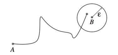
Figure 1: Approximate Controllability Condition. The condition states that given $A,B\in M$ and $\epsilon>0$, there exists $t>0$ and $\phi\in C^{0}([0,t],\mathbb{R}^{p})$ so that $F_{t}\big{(}A,(\phi_{s}-\phi_{0})_{0\leq s\leq t}\big{)}\in\mathcal{B}(B,\epsilon)$.

Condition 2.3.

For all $0\leq t$, the mapping $(x,\phi)\mapsto F_{t}\big{(}x,(\phi_{s}-\phi_{0})_{0\leq s\leq t}\big{)}$ is continuous with respect to the norm $\|x-y\|+\|\phi-\psi\|$ where $\|\phi-\psi\|:=\sup_{0\leq s\leq t}|\phi_{s}-\phi_{0}-(\psi_{s}-\psi_{0})|$.

Let $\phi,\varphi^{1},\ldots,\varphi^{n}$ be $n+1$ deterministic continuous mappings from $[0,t]$ onto $\mathbb{R}^{n}$ equal to $0$ at time $0$. For $\lambda\in\mathbb{R}^{n}$, write

$$G(a,\phi,\lambda):=F_{t}\big{(}a,(\phi_{s}+\sum_{i=1}^{n}\lambda_{i}\varphi^{i}_{s})_{0\leq s\leq t}\big{)}$$ (2.4)

Condition 2.4.

There exists $x_{0}\in M$ and $t>0$, such that in a neighborhood of $(x_{0},0,0)$:

• $(x,(\phi)_{0\leq s\leq t},\lambda)\rightarrow G(x,(\phi)_{0\leq s\leq t},\lambda)$ is differentiable in $\lambda$.

• $\nabla_{\lambda}G$ is invertible and uniformly bounded.

• $(\nabla_{\lambda}G)^{-1}$ is uniformly bounded.

3 Main theorem

Theorem 3.1.

Consider a stochastic process $X_{t}$ on a manifold $M$ that satisfies conditions 2.2, 2.3, 2.4, 2.1 and admits an invariant measure $\mu$. Let $P_{t}$ be the semigroup associated to $X$. Then

• $\mu$ is ergodic and weakly mixing with respect to $P_{t}$.

• $\mu$ is the unique invariant measure of $X$.

Proof.

We will need the following two lemmas on the Levy process $\omega$.

Lemma 3.1.

Assume that $\omega$ satisfies condition 2.1. Let $0\leq s<t$ and $\phi\in C^{0}([0,t],\mathbb{R}^{p})$ be arbitrary. The laws of $\big{(}\omega_{s}-\omega_{0}\big{)}_{0\leq s\leq t}$ and $\big{(}\omega_{s}-\omega_{0}-(\phi_{s}-\phi_{0})\big{)}_{0\leq s\leq t}$ are absolutely continuous with respect to each other.

Proof.

Lemma 3.1 follows by applying Girsanov’s theorem to the diffusive component ($B$) of $\omega$. ∎

Lemma 3.2.

Assume that $\omega$ satisfies condition 2.1. Let $\phi\in C^{0}([0,t],\mathbb{R}^{p})$. For all $\epsilon>0$, the inequality $\mathbb{P}\big{[}\sup_{0\leq s\leq t}|\phi_{s}-\phi_{0}-(\omega_{s}-\omega_{0})|<\epsilon\big{]}>0$ holds almost surely.

Proof.

Let $\epsilon>0$. Let $(\gamma,\sigma,\nu)$ be the Levy-Khintchine characteristics of $\omega$. Let $\eta>0$ such that

$$\int_{z\in\mathbb{R}^{p}\,:\,0<|z|\leq\eta}z^{2}\nu(dz)<\frac{\epsilon^{4}}{16}$$ (3.1)

Observe that [12] can be written as

$$\omega_{t}=\gamma^{\eta}t+\sigma B_{t}+C_{t}^{\eta}+M_{t}^{\eta}$$ (3.2)

where

$$\gamma^{\eta}=\gamma-\int_{z\in\mathbb{R}^{p}\,:\,\eta<|z|\leq 1}z\nu(dz),$$ (3.3)

and

$$C_{t}^{\eta}=\sum_{s\leq t}\Delta_{s}1_{|\Delta_{s}|>\eta}$$ (3.4)

is a compound Poisson point process (of jumps of norm larger than one) and

$$M_{t}^{\eta}=\lim_{\epsilon\downarrow 0}\Big{(}\Delta_{s}1_{\epsilon<|\Delta s|\leq\eta}-t\int_{z\in\mathbb{R}^{p}\,:\,\epsilon<|z|\leq\eta}z\nu(dz)\Big{)}$$ (3.5)

is a martingale (of small jumps compensated by a linear drift). Observe that with strictly positive probability $\exp(-t\nu(|z|>\eta))$, $C_{t}^{\eta}$ is uniformly equal to 0 over $[0,t]$. Furthermore by the Martingale maximal inequality

$$\mathbb{E}[\sup\{(M^{\eta}_{s})^{2}\,:\,0\leq s\leq t\}]\leq 4\mathbb{E}[(M^{\eta}_{t})^{2}]$$ (3.6)

and using ([12])

$$\mathbb{E}[(M^{\eta}_{t})^{2}]=\int_{z\in\mathbb{R}^{p}\,:\,0<|z|\leq\eta}z^{2}\nu(dz)$$ (3.7)

and Chebyshev’s inequality we obtain that

$$\mathbb{P}[\sup_{0\leq s\leq t}|M_{s}|\geq\frac{\epsilon}{2}]\leq\frac{\epsilon}{2}$$ (3.8)

hence

$$\mathbb{P}[\sup_{0\leq s\leq t}|M_{s}|<\frac{\epsilon}{2}]\geq 1-\frac{\epsilon}{2}.$$ (3.9)

We conclude the proof of lemma 3.2 by applying Schilder’s theorem to $B_{t}$ and using the fact that $\sigma$ is not degenerate. ∎

Let us now prove that $\mu$ is ergodic. Let $A\in\mathcal{B}(M)$ be an invariant set of positive $\mu$-measure, i.e.,

$$P_{t}1_{A}=1_{A},\quad\text{for every}\quad t\geq 0,\quad\mu-a.s.$$ (3.10)

and $\mu(A)>0$. We will prove that $\mu(A)=1$. Assume $0<\mu(A)<1$. Then $A^{c}$, which is also an invariant set, has strictly positive measure, i.e. $\mu(A^{c})>0$. Now let us prove the following lemma

Lemma 3.3.

If $0<\mu(A)<1$ then

• For all $y\in M$ and $\epsilon>0$, $\mu(A\cap\mathcal{B}(y,\epsilon))>0$.

• For all $y\in M$ and $\epsilon>0$, $\mu(A^{c}\cap\mathcal{B}(y,\epsilon))>0$.

Proof.

We will restrict the proof to $A$. Since $\mu(A)>0$ there exists $x_{0}>0$ such that for all $\epsilon>0$, $\mu(A\cap\mathcal{B}(x_{0},\epsilon))>0$ (otherwise one would get $\mu(A)=0$ by covering the separable manifold $M$ with a countable number of balls such that $\mu(A\cap\mathcal{B}(x,\epsilon_{x}))=0$). Assume that there exists $y_{0}\in M$ and $\epsilon>0$ such that $\mu(A\cap\mathcal{B}(y_{0},\epsilon))=0$. Since $X_{t}$ is weakly controllable (condition 2.2) there exists $t>0$ and $\phi\in C^{0}([0,t],\mathbb{R}^{p})$ so that $F_{t}\big{(}x_{0},(\phi_{s}-\phi_{0})_{0\leq s\leq t}\big{)}\in\mathcal{B}(y_{0},\frac{\epsilon}{2})$. From the continuity condition 2.3 on $F$ and the Schilder type lemma 3.2 imply that there exists $\epsilon^{\prime}>0$ such that

$$\text{for all}\quad x\in\mathcal{B}(x_{0},\epsilon^{\prime}),\quad\mathbb{P}\big{[}F_{t}\big{(}x,(\phi_{s}-\phi_{0})_{0\leq s\leq t}\big{)}\in\mathcal{B}(y_{0},\epsilon)\big{]}>0.$$ (3.11)

Write $P_{t}$ the semi-group associated with $X_{t}$. Equation (3.11) leads to a contradiction with the fact that

$$\int_{A}P_{t}(x,A)\mu(dx)=\mu(A).$$ (3.12)

since $\mu\big{(}A\cap\mathcal{B}(x_{0},\epsilon^{\prime})\big{)}>0$ and for all $x\in\mathcal{B}(x_{0},\epsilon^{\prime})$, $P_{t}(x,A)<1$.

∎

From condition 2.4 there exists $x_{0}\in M$ and $t,\epsilon,\alpha,\delta,K>0$ and such that for $x\in B(x_{0},\epsilon)$, $\|\phi\|_{L^{\infty}(0,t)}<\alpha$ and $\lambda\in(-\delta,\delta)^{n}$, $G(x,(\phi)_{0\leq s\leq t},\lambda)$ is differentiable in $\lambda$, $|\nabla_{\lambda}G|\leq K$ and $\big{|}(\nabla G)^{-1}\big{|}\leq K$. It follows from the condition 2.4 and the continuity condition 2.3 that $\epsilon^{\prime}\in(0,\epsilon)$ can be chosen small enough so that there exists $z\in M$, $0<\alpha^{\prime}<\alpha$, $0<\epsilon_{z}$ such that for $\|\phi\|_{L^{\infty}(0,t)}<\alpha^{\prime}$ we have for all $a,b\in B(x_{0},\epsilon^{\prime})$,

$$\mathcal{B}(z,\epsilon_{z})\subset G(a,(\phi)_{0\leq s\leq t},(-\delta,\delta)^{n})\cap G(b,(\phi)_{0\leq s\leq t},(-\delta,\delta)^{n}).$$ (3.13)

Equation (3.13) is illustrated in Fig. 2.

Figure 2: Closure Under Second Randomization Condition Illustrated. This condition states that under a second randomization of the noise via $\lambda$, the interior of the intersection of the range of $G(A,\lambda)$ (image of $(-\delta,\delta)^{n}$ by $\lambda\rightarrow G(A,.)$) and $G(B,\lambda)$ is not void.

Let $T>t$. From the previous lemma there exists $a\in\mathcal{B}(x_{0},\epsilon^{\prime})\cap A$ and $b\in\mathcal{B}(x_{0},\epsilon^{\prime})\cap A^{c}$ such that $P_{T}(a,A)=1$ and $P_{T}(b,A^{c})=1$. Set $X_{t}^{a}$ ($X_{t}^{b}$) to be the process $X_{t}$ started from the point $a\in M$ ($b\in M$) and set $\mathbb{P}_{a}$ to be the measure of probability associated to $X_{t}^{a}$. We obtain from the Markov property that

$$\mathbb{E}\big{[}P_{T-t}(X^{a}_{t},A)\big{]}=1\quad\text{and}\quad\mathbb{E}\big{[}P_{T-t}(X^{b}_{t},A)\big{]}=0\text{.}$$ (3.14)

Write

$$X^{a,\lambda}:=F_{t}\big{(}a,(\omega_{s}-\omega_{0}+\sum_{i=1}^{n}\lambda_{i}\varphi^{i}_{s})_{0\leq s\leq t}\big{)}$$ (3.15)

The Girsanov type lemma 3.1 implies that the laws of $X^{a}$ and $X^{a,\lambda}$ are absolutely continuous with respect to each other. Hence for all $\lambda\in(-\delta,\delta)^{n}$,

$$\mathbb{E}\big{[}P_{T-t}(X^{a,\lambda}_{t},A)\big{]}=1\quad\text{and}\quad\mathbb{E}\big{[}P_{T-t}(X^{b,\lambda}_{t},A)\big{]}=0.$$ (3.16)

Which leads to

$$\delta^{-2n}\int_{[-\delta,\delta]^{n}}\mathbb{E}\big{[}P_{T-t}(X^{a,\lambda}_{t},A)\big{]}\,d\lambda=1\quad\text{and}\quad\delta^{-2n}\int_{[-\delta,\delta]^{n}}\mathbb{E}\big{[}P_{T-t}(X^{b,\lambda}_{t},A)\big{]}\,d\lambda=0.$$ (3.17)

Let $\Omega_{I}$ be the event $\|\omega\|_{L^{\infty}(0,t)}<\alpha^{\prime}$. Observe that from the Schilder type lemma 3.2 the measure of probability of $\Omega_{I}$ is strictly positive. It follows from (3.17) and (3.13) that

$$\delta^{-2n}\int_{[-\delta,\delta]^{n}}\mathbb{E}\big{[}1_{\Omega_{I}}1_{X^{a,\lambda}_{t}\in\mathcal{B}(z,\epsilon_{z})}P_{T-t}(X^{a,\lambda}_{t},A)\big{]}\,d\lambda>0$$ (3.18)

Using the change of variable $y=X^{a,\lambda}_{t}$ we obtain from (3.13) that

$$\mathbb{E}\big{[}1_{\Omega_{I}}\int_{\mathcal{B}(z,\epsilon_{z})}P_{T-t}(y,A)\frac{dy}{|\nabla_{\lambda}X^{a,\lambda}|\circ(X^{a,\lambda})^{-1}(y)}\big{]}>0$$ (3.19)

Hence

$$\mathbb{E}\big{[}1_{\Omega_{I}}\int_{\mathcal{B}(z,\epsilon_{z})}P_{T-t}(y,A)\frac{|\nabla_{\lambda}X^{b,\lambda}|\circ(X^{b,\lambda})^{-1}(y)}{|\nabla_{\lambda}X^{a,\lambda}|\circ(X^{a,\lambda})^{-1}(y)}\frac{dy}{|\nabla_{\lambda}X^{b,\lambda}|\circ(X^{b,\lambda})^{-1}(y)}\big{]}>0$$ (3.20)

We deduce from equation (3.13) and the fact that $\frac{|\nabla_{\lambda}X^{b,\lambda}|\circ(X^{b,\lambda})^{-1}(y)}{|\nabla_{\lambda}X^{a,\lambda}|\circ(X^{a,\lambda})^{-1}(y)}$ is bounded from below by $K^{-2}$ that

$$\mathbb{E}\big{[}1_{\Omega_{I}}\int_{\mathcal{B}(z,\epsilon_{z})}P_{T-t}(y,A)\frac{dy}{|\nabla_{\lambda}X^{b,\lambda}|\circ(X^{b,\lambda})^{-1}(y)}\big{]}>0.$$ (3.21)

However a similar computation leads from (3.17) and (3.13) to

$$\mathbb{E}\big{[}1_{\Omega_{I}}\int_{\mathcal{B}(z,\epsilon_{z})}P_{T-t}(y,A)\frac{dy}{|\nabla_{\lambda}X^{b,\lambda}|\circ(X^{b,\lambda})^{-1}(y)}\big{]}=0.$$ (3.22)

Hence a contradiction. Thus $\mu$ must be ergodic. Let us now prove that $\mu$ is the unique invariant measure. Assume that $\mu^{\prime}\not=\mu$ is also invariant with respect to the semigroup $P_{t}$. By the argument presented above $\mu^{\prime}$ is ergodic and it follows from Proposition 3.2.5 of [10] that $\mu$ and $\mu^{\prime}$ are singular and it is easy to check from the argument presented above that this can’t be the case (the proof is similar to the one given in theorem 4.2.1 of [10]). Hence $\mu$ is the unique invariant distribution. The proof of the fact that $\mu$ is weakly mixing follows from theorem 3.4.1 of [10] and is similar to the one given at page 44 of [10] (theorem 4.2.1). ∎

4 Sliding Disk at Uniform Temperature.

Consider a disk on a surface as shown in Fig. 3 [1]. The disk is free to slide and rotate. We assume that one rescales position its radius and time by some characteristic frequency of rotation or other time-scale. The dimensionless Lagrangian is given by

$$L(x,v,\theta,\omega)=\frac{1}{2}v^{2}+\frac{\sigma}{2}\omega^{2}-U(x)$$ (4.1)

where $v$ stands for the velocity of the center of mass, $\omega$ the angular velocity of the disk and $\sigma$ is a strictly positive dimensionless constant given by $\sigma:=J/(mr^{2})$ (where $r$ is the radius of the disk, $m$ is its mass and $J$ its moment of inertia). $U:\mathbb{R}\to\mathbb{R}$ is an arbitrary periodic potential which is assumed to be smooth, and of period one.

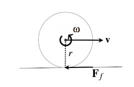
Figure 3: Sliding Disk. Consider a sliding disk of radius $r$ that is free to translate and rotate on a surface. We assume the disk is in sliding frictional contact with the surface. The configuration space of the system is $\operatorname{SE}(2)$, but with the surface constraint the configuration space is just $\mathbb{R}\times\operatorname{SO}(2)$.

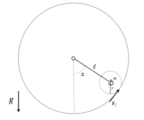
Figure 4: Ballistic Pendulum. If the dimensionless potential is $U=\cos(x)$, then the sliding disk is simply a pendulum in which the bob in the pendulum is replaced by a disk and the pendulum is placed within a cylinder as shown.

The contact with the surface is modeled using a sliding friction law. For this purpose we introduce a symmetric matrix $\mathbf{C}$ defined as,

$$\mathbf{C}=\begin{bmatrix}1&1/\sigma\\ 1/\sigma&1/\sigma^{2}\end{bmatrix}\text{.}$$

Observe that $\mathbf{C}$ is degenerate since the frictional force is actually applied to only a single degree of freedom, and hence, one of its eigenvalues is zero. In addition to friction a white noise is applied to the same degree of freedom to which friction is applied. The governing stochastic differential equations are

$$\begin{cases}dx&=vdt\\ d\theta&=\omega dt\\ \begin{bmatrix}dv\\ d\omega\end{bmatrix}&=\begin{bmatrix}-\partial_{x}U\\ 0\end{bmatrix}dt-c\mathbf{C}\begin{bmatrix}v\\ \sigma\omega\end{bmatrix}dt+\alpha\mathbf{C}^{1/2}\begin{bmatrix}dB_{v}\\ dB_{\omega}\end{bmatrix}\text{.}\end{cases}$$ (4.2)

where $\mathbf{C}^{1/2}$ is the matrix square root of $\mathbf{C}$. The matrix square root is easily computed by diagonalizing $\mathbf{C}$ and computing square roots of the diagonal entries (eigenvalues of $\mathbf{C}$) as shown:

$$\mathbf{C}^{1/2}=\frac{\sigma}{\sqrt{\sigma^{2}+1}}\mathbf{C}\text{.}$$

Write $X:=(x,\theta,v,\omega)$. It easy to check that the Gibbs distribution

$$\mu(d\xi):=\frac{e^{-\beta E}}{Z}dX$$ (4.3)

is invariant for (4.2), where $\beta=2c/\alpha^{2}$, $Z:=\int e^{-\beta E}dX$, and $E$ is the energy of the mechanical system and is given by

$$E:=\frac{1}{2}v^{2}+\frac{1}{2}\sigma\omega^{2}+U(x)\text{.}$$

Define

$$Y:=\begin{pmatrix}-x+\sigma\theta\\ x+\theta\end{pmatrix}$$ (4.4)

The system (4.2) can be written

$$\begin{cases}\dot{Y_{1}}(t)=\dot{Y_{1}}(0)+\int_{0}^{t}\partial_{x}U(\frac{\sigma Y_{2}-Y_{1}}{\sigma+1})\,ds\\ \dot{Y_{2}}(t)=\dot{Y_{2}}(0)-\int_{0}^{t}\partial_{x}U(\frac{\sigma Y_{2}-Y_{1}}{\sigma+1})\,ds-c\gamma(Y_{2}(t)-Y_{2}(0))+\bar{\alpha}\sqrt{2}B_{t}\end{cases}$$ (4.5)

where $\gamma=(\sigma+1)/\sigma$, $\bar{\alpha}=\alpha(\sigma+1)/\sqrt{\sigma^{2}+1}$ and $B:=(B_{v}+B_{\omega})/\sqrt{2}$ is a one dimensional Brownian Motion. Observe that condition 2.1 is satisfied with $\omega=B$, $p=1$ and $\sigma=(1)$.

Observe also that if $U$ is a constant then the quantity $-v+\sigma\omega$ is conserved and the system (4.2) can’t be ergodic. Let us assume that $U$ is not constant, our purpose is to prove that the Gibbs distribution $\mu$ is ergodic with respect to the stochastic process $X$.

Remark 4.1.

Observe that when $U$ is not constant over a non void open subset of $\mathbb{R}$ (say $(-\frac{1}{4},\frac{1}{4})$), $Y$ needs to travel a distance that is uniformly (in $\epsilon$) bounded from below by a strictly positive amount to get from $(Y_{1},Y_{2},\dot{Y_{1}},\dot{Y_{2}})=(0,0,0,0)$ to the domain $\dot{Y_{1}}>\epsilon$. It follows that in that situation that the process $Y$ and hence $X$ is not strong Feller and theorems requiring this property can’t be applied.

Remark 4.2.

Observe also that the condition $\partial_{x}^{2}U\not=0$ in a neighborhood of $x_{0}$ doesn’t guarantee that $Y$ is strongly Feller in that neighborhood. For instance observe that $\partial_{x}^{2}U(x_{0})\not=0$ and $\partial U(x_{0})>0$ imply that the drift on $Y_{1}$ is uniformly bounded by a strictly positive constant on a neighborhood of $(0,\frac{\sigma+1}{\sigma}x_{0})$ it follows that $\mathbb{P}_{\epsilon}{(y_{1},y_{2})}[Y_{1}<0]$ is discontinuous in the neighborhood of $(0,\frac{\sigma+1}{\sigma}x_{0})$ ($\epsilon$) close to the line $y_{1}=0$.

We believe that the system $Y$ is asymptotically strong Feller so one could in principle obtain the ergodicity of $\mu$ by controlling the semi-group associated to $Y$ as it is suggested in [6]. We propose an alternative method based on the controllability of the ODE associated to $Y$ and theorem 3.1. We believe that it is much simpler to control the geometric properties of the ODE associated to $X$ rather than the gradient of its semigroup.

One can also check that the generator of $Y$ satisfies a local Hörmander condition ([11] 38.16) at a point $x_{0}$ such that $\partial_{x}^{2}U(x_{0})\not=0$ so an alternative method to prove ergodicity would be to use that condition to obtain a local regularity of the semi group associated to $U$. Here we propose an alternative method which doesn’t require $U$ to be smooth and which can be applied with Levy processes.

Theorem 4.1.

Assume that $U$ is not constant. Then the Gibbs measure $\mu$ is ergodic and strongly mixing with respect to the stochastic process $X$ (4.2). Furthermore, it is the unique invariant distribution of $X$.

First let us prove that codition 2.2 is satisfied by $X$.

Lemma 4.1.

Assume $U$ is not constant. Then $Y$ is approximately controllable.

Proof.

Since $U$ is not constant, there exists $t_{1}>0$ such that for $t_{i}\geq t_{1}$ there exists a smooth path $Y$ such that $Y_{1}(0)=-x_{1}+\sigma\theta_{1}$, $Y_{2}(0)=x_{1}+\theta_{1}$, $\dot{Y_{1}}(0)=-v_{1}+\sigma\omega_{1}$, $\dot{Y_{2}}(0)=v_{1}+\omega_{1}$, $Y_{1}(t_{i})=-x_{2}+\sigma\theta_{2}$, $\dot{Y_{1}}(t_{i})=-v_{2}+\sigma\omega_{2}$ and

$$\frac{d^{2}Y_{1}}{dt^{2}}=\partial_{x}U\left(\frac{\sigma Y_{2}-Y_{1}}{\sigma+1}\right)$$ (4.6)

Take $t_{2}:=t_{i}+\frac{\min(\epsilon,1)}{10(\|\partial_{x}U\|_{L^{\infty}}+1+|\frac{d}{dt}Y_{1}(t_{i})|)}$ and interpolate smoothly $Y_{2}$ between $Y_{2}(t_{i})$ (obtained from the control problem (4.6)) and

$$\begin{pmatrix}Y_{2}(t_{2})\\ \frac{dY_{2}}{dt}(t_{2})\end{pmatrix}=\begin{pmatrix}x_{2}+\theta_{2}\\ v_{2}+\omega_{2}\end{pmatrix}$$ (4.7)

Observe that the extension of $Y_{1}$ to $(t_{i},t_{2}]$ as a solution of (4.6) satisfies

$$\Big{|}\begin{pmatrix}Y_{1}(t_{2})-Y_{1}(t_{i})\\ \frac{dY_{1}}{dt}(t_{2})-\frac{dY_{1}}{dt}(t_{i})\end{pmatrix}\Big{|}\leq\frac{\epsilon}{5}$$ (4.8)

Taking $\phi$ be the smooth curve defined by $\phi(0)=0$ and

$$\frac{d^{2}Z_{2}}{dt^{2}}=-\partial_{x}U\left(\frac{\sigma Z_{2}-Z_{1}}{\sigma+1}\right)-c\gamma\frac{dZ_{2}}{dt}+\bar{\alpha}\sqrt{2}\frac{d\phi}{dt}$$ (4.9)

completes the proof. ∎

Proof.

The proof that $X$ satisfies condition 2.3 is a standard application of Gronwall’s lemma. Observe that the semi-group associated to $X$ is not strongly irreducible and never equivalent to $\mu$ because $|(-v+\sigma\omega)(t)-(-v+\sigma\omega)(0)|\leq\|\partial_{x}U\|_{L^{\infty}}t$. Let us now show that condition 2.4 is satisfied.

Write $\xi$ the stochastic process defined by

$$\begin{cases}\dot{\xi_{1}}(t)=\dot{\xi_{1}}(0)+\int_{0}^{t}\partial_{x}U(\frac{\sigma\xi_{2}-\xi_{1}}{\sigma+1})\,ds\\ \dot{\xi_{2}}(t)=\dot{\xi_{2}}(0)+\bar{\alpha}\sqrt{2}B_{t}\end{cases}$$ (4.10)

To prove that $Y$ satisfies condition 2.4 it is sufficient to show that $\xi$ satisfies condition 2.4.

Since $U$ is smooth and not constant, there exists a point $x^{0}\in[0,1)$, $\epsilon,C>0$ such that for $x\in B(x^{0},\epsilon)$, $\partial_{x}^{2}U>C$. Let $\zeta$ be a point of the phase space such that $\frac{\sigma\zeta_{2}-\zeta_{1}}{\sigma+1}=x^{0}$ and $\dot{\zeta}_{1}=\dot{\zeta}_{2}=0$. Let $0<\epsilon^{\prime}<\epsilon/100$ and $a\in B(\zeta,\epsilon^{\prime})$.

Let $\varphi_{1},\ldots,\varphi_{4}$ be $4$ continuous mappings from $\mathbb{R}^{+}$ onto $\mathbb{R}$, equal to zero at time zero. For $\lambda\in\mathbb{R}^{4}$ we write $\xi^{\lambda}$ the solution of

$$\begin{cases}\dot{\xi_{1}^{\lambda}}(t)=\dot{a}_{1}+\int_{0}^{t}\partial_{x}U(\frac{\sigma\xi_{2}^{\lambda}-\xi_{1}^{\lambda}}{\sigma+1})\,ds\\ \dot{\xi_{2}^{\lambda}}(t)=\dot{a}_{2}+\bar{\alpha}\sqrt{2}\sum_{i=1}^{4}\lambda_{i}\varphi_{i}(t)\\ \xi_{1}^{\lambda}(t)=a_{1}+\int_{0}^{t}\dot{\xi_{1}^{\lambda}}(s)\,ds\\ \xi_{2}^{\lambda}(t)=a_{2}+\int_{0}^{t}\dot{\xi_{2}^{\lambda}}(s)\,ds\end{cases}$$ (4.11)

It follows that

$$\begin{cases}\dot{\xi_{1}^{\lambda}}(t)-\dot{\xi_{1}^{0}}(t)=\int_{0}^{t}(\frac{\sigma\xi_{2}^{\lambda}-\xi_{1}^{\lambda}}{\sigma+1}-\frac{\sigma\xi_{2}^{0}-\xi_{1}^{0}}{\sigma+1})\int_{0}^{1}\partial_{x}^{2}U\big{(}\frac{\sigma\xi_{2}^{0}-\xi_{1}^{0}}{\sigma+1}+\alpha(\frac{\sigma\xi_{2}^{\lambda}-\xi_{1}^{\lambda}}{\sigma+1}-\frac{\sigma\xi_{2}^{0}-\xi_{1}^{0}}{\sigma+1})\big{)}(s)\,ds\,d\alpha\\ \dot{\xi_{2}^{\lambda}}(t)-\dot{\xi_{2}^{0}}(t)=\sum_{i=1}^{4}\lambda_{i}\big{(}\bar{\alpha}\sqrt{2}\varphi_{i}(t)\big{)}\\ \xi_{1}^{\lambda}(t)-\xi_{1}^{0}(t)=\int_{0}^{t}(\dot{\xi_{1}^{\lambda}}(s)-\dot{\xi_{1}^{0}}(s))\,ds\\ \xi_{2}^{\lambda}(t)-\xi_{2}^{0}(t)=\sum_{i=1}^{4}\lambda_{i}\big{(}\bar{\alpha}\sqrt{2}\int_{0}^{t}\varphi_{i}(s)\,ds\big{)}\end{cases}$$ (4.12)

Writing $\eta$ the solution of

$$\begin{cases}\dot{\eta}(t)+\frac{\partial_{x}^{2}U\big{(}x^{0}\big{)}}{\sigma+1}\int_{0}^{t}\eta(s)\,ds=\partial_{x}^{2}U\big{(}x^{0}\big{)}\frac{\sigma}{\sigma+1}\int_{0}^{t}(\xi_{2}^{\lambda}-\xi_{2}^{0})(s)\,ds\\ \eta=\int_{0}^{t}\dot{\eta}(s)\,ds\end{cases}$$ (4.13)

we obtain that up to the first order in $\lambda$, and at the order $0$ in $\epsilon^{\prime}$ and $t$, $\big{(}\dot{\xi_{1}^{\lambda}}(t)-\dot{\xi_{1}^{0}}(t),\xi_{1}^{\lambda}(t)-\xi_{1}^{0}(t)\big{)}$ can be approximated by $(\dot{\eta}(t),\eta(t))$. It follows that $\xi^{\lambda}_{t}-\xi^{0}_{t}$ can be written as $M(\lambda,t)\lambda$ where $M(\lambda,t)$ is continuous in $t$ and $\lambda$ in the neighborhood of $0$. Moreover, $\varphi_{1},\ldots,\varphi_{4}$ can be chosen so that $M$, and $M^{-1}$ are uniformly bounded in that neighborhood. Choosing $0<\delta\ll 1$ and $0<\epsilon^{\prime}\ll\delta t\ll 1$ implies condition 2.4. By invoking theorem 3.1 one obtains that the process is ergodic and weakly mixing.

It follows from theorem 3.4.1 of [10] that for $\varphi\in L^{2}(\mu)$ there exists a set $I\subset[0,+\infty)$ of relative measure $1$ such that

$$\lim_{|t|\rightarrow\infty,\;t\in I}\mathbb{E}[\varphi(x_{t},\theta_{t},v_{t},\omega_{t})]=\mu[\varphi]\quad\text{in}\quad L^{2}(\mu)\text{.}$$ (4.14)

Furthermore since $t\rightarrow\mathbb{E}[\varphi(x_{t},\theta_{t},v_{t},\omega_{t})]$ is continuous when $\varphi$ is continuous and bounded we deduce that when $\varphi$ is continuous and bounded then

$$\lim_{t\rightarrow\infty}\mathbb{E}[\varphi(x_{t},\theta_{t},v_{t},\omega_{t})]=\mu[\varphi]\quad\text{in}\quad L^{2}(\mu)\text{.}$$ (4.15)

The fact that the process is strongly mixing then follows from corollary 3.4.3 of [10]. ∎

In [1], using thoerem 4.1 we prove that if $U$ is non-constant then the $x$-displacement of the sliding disk is $\mu$ a.s. not ballistic (see Proposition 4.1). However, the mean-squared displacement with respect to the invariant law is ballistic (see theorem 4.2). More precisely, we show that the squared standard deviation of the $x$-displacement with respect to its noise-average grows like $t^{2}$. This implies that the process exhibits not only ballistic transport but also ballistic diffusion. If $U$ is constant then the squared standard deviation of the $x$-displacement is diffusive (grows like $t$). See below for theoretical results and numerical experiments using efficient stochastic variational integrators.

Proposition 4.1.

Provided that $U$ is non-constant, then $\mu$ a.s.

$$\lim_{t\to\infty}\frac{x(t)-x(0)}{t}\to 0\text{.}$$

Proposition 4.2.

The squared standard deviation of the $x_{t}+\theta_{t}$-degree of freedom is diffusive, i.e.,

$$\lim_{t\rightarrow\infty}\frac{\mathbb{E}_{\mu}[(x_{t}+\theta_{t}-\mathbb{E}[x_{t}+\theta_{t}])^{2}]}{t}=\frac{2\alpha^{2}\sigma^{2}}{c^{2}(\sigma^{2}+1)}\text{.}$$ (4.16)

Proposition 4.3.

Assume that $U$ is non constant, then

$$\lim\sup_{t\rightarrow\infty}\frac{\mathbb{E}_{\mu}\Big{[}\big{(}-x_{t}+\sigma\theta_{t}-\mathbb{E}[-x_{t}+\sigma\theta_{t}]\big{)}^{2}\Big{]}}{t^{2}}\leq 4\frac{1+\sigma}{\beta}$$ (4.17)

and

$$\lim\inf_{t\rightarrow\infty}\frac{\mathbb{E}_{\mu}\Big{[}\big{(}-x_{t}+\sigma\theta_{t}-\mathbb{E}[-x_{t}+\sigma\theta_{t}]\big{)}^{2}\Big{]}}{t^{2}}\geq\frac{1}{4}\frac{1+\sigma}{\beta}$$ (4.18)

Theorem 4.2.

We have ([1])

• If $U$ is constant then

  $$\lim_{t\rightarrow\infty}\frac{\mathbb{E}_{\mu}\big{[}(x_{t}-\mathbb{E}[x_{t}])^{2}\big{]}}{t}=\frac{2\alpha^{2}\sigma^{2}}{c^{2}(\sigma^{2}+1)(\sigma+1)^{2}}$$ (4.19)

• If $U$ is non constant then

  $$\lim\sup_{t\rightarrow\infty}\frac{\mathbb{E}_{\mu}\big{[}(x_{t}-\mathbb{E}[x_{t}])^{2}\big{]}}{t^{2}}\leq\frac{4}{\beta(1+\sigma)}$$ (4.20)

  and

  $$\lim\inf_{t\rightarrow\infty}\frac{\mathbb{E}_{\mu}\big{[}(x_{t}-\mathbb{E}[x_{t}])^{2}\big{]}}{t^{2}}\geq\frac{1}{4\beta(1+\sigma)}$$ (4.21)

Classical homogenization techniques can’t be applied to obtain theorem 4.2 (since the stochastic forcing is degenerate on momentums). We refer to [1] for a proof of that theorem. The ballistic diffusion is caused by long time memory effects created by the degeneracy of the noise and the coupling between the two degrees of freedom through $U$. Figure 5 gives an illustration of the mean-squared displacement of the rolling disk versus time started from rest. In [1] we have used that phenomenon to propose a fluctuation driven magnetic motor characterized by ballistic diffusion at uniform. A plot of the angular displacement of that magnetic motor versus time for a single realization started from rest is given in figure 6.

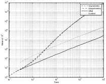
Figure 5: Sliding Disk at Uniform temperature, $h=0.01$, $\alpha=5.0$, $c=0.1$. A log-log plot of the mean squared displacement of the ball. It clearly shows that the x-position exhibits anomalous diffusion when $U$ is symmetric or asymmetric. The disk is started from rest. In the control and flat $U$ cases the diffusion is normal.

     (a) $\alpha=0.001$         (b) $\alpha=0.001$         (c) $\alpha=0.00075$         (d) $\alpha=0.00075$

Figure 6: Angular position of a magnetic motor (uniform temperature). Four different realizations of the angular component of the center of mass of a magnetic motor are plotted. The system is started from rest.

References

• [1] N. Bou-Rabee and H. Owhadi. Ballistic transport at uniform temperature. Submitted; arXiv:0710.1565, 2007.
• [2] J.-P. Eckmann and M. Hairer. Non-equilibrium statistical mechanics of strongly anharmonic chains of oscillators. Comm. Math. Phys., 212(1):105–164, 2000.
• [3] J.-P. Eckmann and M. Hairer. Uniqueness of the invariant measure for a stochastic PDE driven by degenerate noise. Comm. Math. Phys., 219(3):523–565, 2001.
• [4] J.-P. Eckmann, C.-A. Pillet, and L. Rey-Bellet. Non-equilibrium statistical mechanics of anharmonic chains coupled to two heat baths at different temperatures. Comm. Math. Phys., 201(3):657–697, 1999.
• [5] Jean-Pierre Eckmann, Claude-Alain Pillet, and Luc Rey-Bellet. Entropy production in nonlinear, thermally driven Hamiltonian systems. J. Statist. Phys., 95(1-2):305–331, 1999.
• [6] Martin Hairer and Jonathan C. Mattingly. Ergodicity of the 2D Navier-Stokes equations with degenerate stochastic forcing. Ann. of Math. (2), 164(3):993–1032, 2006.
• [7] J. C. Mattingly and A. M. Stuart. Geometric ergodicity of some hypo-elliptic diffusions for particle motions. Markov Process. Related Fields, 8(2):199–214, 2002. Inhomogeneous random systems (Cergy-Pontoise, 2001).
• [8] J. C. Mattingly, A. M. Stuart, and D. J. Higham. Ergodicity for SDEs and approximations: locally Lipschitz vector fields and degenerate noise. Stochastic Process. Appl., 101(2):185–232, 2002.
• [9] Sean Meyn and Richard Tweedie. Markov Chains and Stochastic Stability (Communications and Control Engineering). Springer, 1996.
• [10] G. Da Prato and J. Zabczyk. Ergodicity for infinite dimensional systems. London Mathematic Society Lecture Note Series 229. Cambridge University Press, 1996.
• [11] L.C.G. Roger, D. Williams. Volume 1, and 2. Diffusions, Markov processes and Martingales. Cambridge University Press, 2006.
• [12] Matthias Winkel. Lecture notes on levy processes. http://www.stats.ox.ac.uk/w̃inkel/ms3b.html, 2008.