Crowded-Field Astrometry with the
Space Interferometry Mission - I
Estimating the Single-Measurement Astrometric Bias
Arising from Confusion

Abstract

The accuracy of position measurements on stellar targets with the future Space Interferometry Mission (SIM) will be limited not only by photon noise and by the properties of the instrument (design, stability, etc.) and the overall measurement program (observing strategy, reduction methods, etc.), but also by the presence of other “confusing” stars in the field of view (FOV). We use a simple “phasor” model as an aid to understanding the main effects of this “confusion bias” in single observations with SIM. This analytic model has been implemented numerically in a computer code and applied to a selection of typical SIM target fields drawn from some of the Key Projects already accepted for the Mission. We expect that less than 1% of all SIM targets will be vulnerable to confusion bias; we show that for the present SIM design, confusion may be a concern if the surface density of field stars exceeds 0.4 star/arcsec². We have developed a software tool as an aid to ascertaining the possible presence of confusion bias in single observations of any arbitrary field. Some a priori knowledge of the locations and spectral energy distributions of the few brightest stars in the FOV is helpful in establishing the possible presence of confusion bias, but the information is in general not likely to be available with sufficient accuracy to permit its removal. We discuss several ways of reducing the likelihood of confusion bias in crowded fields. Finally, several limitations of the present semi-analytic approach are reviewed, and their effects on the present results are estimated. The simple model presented here provides a good physical understanding of how confusion arises in a single SIM observation, and has sufficient precision to establish the likelihood of a bias in most cases. We close this paper with a list of suggestions for future work on this subject.

1 Introduction

The Space Interferometry Mission (SIM) is being designed by NASA’s Jet Propulsion Laboratory to provide a facility-class instrument for measuring the positions and proper motions of stars at optical wavelengths with micro-arc-second ($\mu{\rm as}$) precision. This represents an improvement by several orders of magnitude over the precision of all existing astrometric instruments. For faint sources (V $\gtrsim 15$ mag.), SIM will also be more than a factor 10 better than any other future planned space mission, and will therefore uniquely permit many new classes of problems to be addressed. Such problems include: the direct measurement (for the first time) of the masses of earth-like planets in orbit around nearby stars; determining the distances to stars by direct triangulation over the whole Galaxy and out to the Magellanic Clouds; measuring the transverse motions of galaxies in the Local Group; and, establishing the shape of the dark matter distribution in the Galaxy. A description of the instrument and its current science program is available at the JPL/SIM web site. The mission is now at the end of the detailed design phase. After more than 15 years of development, all the major technical questions have been answered. New devices have been invented in order to provide metrology internal to the spacecraft at a level of a few tens of picometers, a fraction of the inter-atomic distance in a molecule of oxygen. The next major step is to begin construction of the instrument.

SIM will be the second optical interferometer in space devoted to astrometry, following the Fine Guidance Sensors (FGS) on the Hubble Space Telescope (HST). However, SIM is a Michelson interferometer using separated collectors, quite different from the filled-aperture white-light shearing interferometer design of the FGS. SIM includes three long-baseline interferometers housed on a common truss, each formed by two $\approx 0.3$ m apertures which compress their light beams and guide them through delay lines to beam combiners. During operation, two interferometers are used for precision guiding of the spacecraft, and the third views the target of interest. Data are then accumulated by tracking the target until enough photons have been recorded to achieve the particular science goal.

The precision with which astrometry can be done on a specific stellar target with SIM will be limited by photon noise, the design and stability of the instrument, and by the data calibration and processing. We have some control over the instrument properties, which depend on the specific choices made when implementing the design in hardware. Also, the operation and calibration of the instrument can be optimized so as to maximize the achievable precision. However, there is another source of error which may be present, and which is largely out of our control; it does not reduce the ultimate precision with which a given single measurement can be made with SIM, but it may reduce the final accuracy of that measurement. This source of error arises because of the presence of other stars in the SIM field of view (FOV) which can “confuse” any single observation made on the target star. The light from these extraneous stars perturbs the measurement, so that the measured target position can differ from the true position. The difference is a bias which can reach a level of many times the single-measurement precision estimated from the instrument parameters alone. It is this single-measurement confusion bias which concerns us in this paper.

It is important to emphasize that the final accuracy of the astrometric parameters (position, parallax, and proper motion) determined by SIM for any given target star will be a result of carrying out a complex program of several single measurements on that target, plus repeated measurements on many other stars for the determination of calibration and baseline orientation parameters (Boden, 2004; Milman & Turyshev, 2003). Since we are concerned only with possible bias in a single measurement, the details of the entire observing program are not directly relevant here; however, it also means that we can not quantify the consequences of confusion bias to the final accuracy with which the “end-of-mission” astrometric parameters can be obtained on any specific target. It is clear that the effects of single-measurement confusion bias will generally diminish as more observations are combined. But this also means that projects which involve only a few observations of a target (e.g. “targets of opportunity”, single parallax measurements on nearby bright stars, etc.) may have a greater susceptibility to confusion bias.

Specific aspects of confusion in astrometric measurements with SIM have been considered by several authors in the recent past. Dalal & Griest (2001) showed that the characteristic response of SIM’s fixed-baseline interferometer as a function of wavenumber and delay can be used to refine a model of the distribution of confusing stars in the FOV. This model can then be used to correct the measured position of the target of interest, and in many cases where the level of confusion is not too great the astrometric accuracy can approach the measurement precision. Dalal and Griest successfully applied their method to models of confused fields in the LMC in which $\approx 16$ faint stars are scattered over the FOV around the $\approx 19$ magnitude target star. Photon noise is included in these models. These authors then go on to consider the additional complication if one of the stars in the FOV changes brightness owing to a micro-lensing event, and show that an extension of their fitting algorithm to include the precision photometry provided by SIM’s detectors permits even this apparently-intractable case to be handled almost as well. However, their method fails when the angular separation between any pair of sources in the FOV (as projected on the interferometer baseline) corresponds to a delay difference of $\lesssim 2$ coherence lengths for the full bandpass of the detection system. This is a projected separation of 25 milli-arcseconds (mas). Indeed, this is a general limit for SIM observations. Our approach is somewhat simpler than that of Dalal and Griest, and yields some improvement in the minimum angular separation which can be measured, but the basic limitation can not be overcome. We will compare our approach to theirs in more detail in a future paper.

Rajagopal et al. (2001) also considered a number of specific cases of confusion on SIM astrometry. These authors introduced a graphical analogy using phasors as an aid to understanding how errors in the target position arise from confusing sources in the FOV. Typical target fields were constructed on a simulated image with grid spacing of 5 mas, and the amplitude and phase of the fringe which would be measured with SIM for a given wavelength on that image field was computed with a Fourier transform. Diffraction effects at the edges of the (presumed $\approx 1^{\prime\prime}$ square) SIM FOV were included in constructing the model image, and vector averaging of the individual (narrow) SIM wavelength channels was used to simulate the 1-dimensional apodization of the fringes over the FOV caused by the decreasing coherence of the fringes as the bandwidth increases. Rajagopal et al. (2001) were particularly interested in modeling the effects of mispointing of the FOV in subsequent visits to the same target field when target proper motions were being measured; in that case the actual distribution of field stars changes as some disappear from one side of the FOV and others appear at the other side. They included photon noise, and also addressed the issue of how the size of the FOV defined by the field stop influenced the level of confusion. Their source field models were constructed to simulate SIM observations of the position and proper motion of target stars in M31, the LMC, and the Galactic bulge. They concluded that the confusion-induced errors in position can often be significant (several times the measurement precision) for faint target stars but the proper motion errors are likely to be small. The errors are, as expected, smaller for wider measurement bands.

In one other confusion-related study, Takeuchi et al. (2005) considered the effect of circumstellar disks on the measurement of stellar wobble during observations aimed at detecting extra-solar planets. Their models showed that neither the motion of the disk mass center nor the contamination by disk light is a serious threat to detecting planets around pre-main sequence stars; the basic reason for the insensitivity of these observations to confusion from circumstellar disks is that interferometers tend to resolve such an extended source, reducing its influence on the astrometry of the parent star.

The studies summarized above have shown that confusion poses limits to the accuracy of any single SIM measurement, and have therefore succeeded in raising our awareness of this problem. However, the detailed design of SIM has changed since those studies were done, and many of the changes will affect on the modeling results. The size of the collector and its central obscuration, the entrance aperture field stop defining the geometrical FOV, the transmission efficiency of the optics, the fringe disperser design (which defines the bandwidth and central wavelength of the spectral channels), and the QE and spectral response of the detector are now all much better defined. Furthermore, previous studies have focused on specific science programs which were already suspected to be pushing the capabilities of the instrument; they have not provided us with any general “tools” for understanding and recognizing confusion, or for dealing with it. Previous studies have also often taken a statistical approach which is less suitable for answering direct questions about specific fields, such as: is a SIM observation of this particular target embedded in that particular field of stars likely to be confused? And, can the observation be done in such a way so as to reduce the confusion bias? What a priori information about the target and the field would help? And, if the observation has already been taken, can we identify the effects of confusion in the data? These questions have provided the motivation for the work described in this paper.

This paper is organized as follows. In the next section, we summarize the basic Michelson interferometer response as it applies to SIM. We then recall the phasor model introduced by Rajagopal et al. (2001) and elaborate upon it as a tool for understanding the behavior of confusion in SIM astrometry. Using this analytic model, together with updated knowledge of SIM’s instrument parameters, we have constructed a simulation code for evaluating the likelihood of confusion bias in any specific field; details are presented in Section 3. In Section 4, we present single measurement confusion bias as a function of magnitude difference and projected separation of an additional star present within the SIM FOV. In Section 5, we apply this semi-analytic model to a number of target fields drawn from the Key Projects which have already been chosen for the initial SIM science program. From this experience we then consider how the single-measurement confusion bias might be reduced through the addition of other information. The most useful additions appear to be knowledge of the approximate locations and spectral energy distributions (SEDs) of the target and of the most troublesome confusing stars in the SIM FOV. Finally, in Section 6, we describe the limitations of our current approach. These limitations are primarily related to the simplified model of the focal plane of SIM which we have used here. In particular, in this paper, we have not modeled the detailed mechanism by which the spectral dispersion is implemented, nor have we considered the pixellation of the focal plane by the CCD detector. We have explored these points with the aid of a more elaborate model that includes these effects, and find that the biases estimated using this more elaborate model differ only by small amounts from those provided by the approach described here. We have therefore chosen to present the main issues relevant to SIM confusion with a minimum of complication, and leave the discussion of the more elaborate instrument model to a future paper.

Binary stars will be an important class of targets for SIM, and are the topic of one of the major Key Projects. In these cases, the two stars are in a bound orbit and are physically close to each other. Typical binaries to be studied with SIM will have separations from about a few mas to 1000 mas and orbital periods from a few days to several years. Stars in crowded fields can occasionally mimic the effects of binaries if their projected separations become small for particular baseline orientations, but the effects of confusion from such “apparent” binaries can be reduced (or even eliminated) by rotating the interferometer baseline and repeating the observation. However, for “real” binaries, rotation of the baseline is an integral part of the measurement process. The goal of the binary observation is to obtain the characteristics of the orbit, and this is done by measuring the positions of the components for a number of baseline orientations. These targets are sufficiently specialized that we have removed them from the list of crowded-field problems treated in this paper. Such observations treat binaries as “signal”, whereas here we treat them as “noise”. A discussion of astrometry on binary stars with SIM is planned for a future publication.

2 Astrometry with SIM

Historically, the angular separation between two stars on the sky has been determined using telescopes of various sizes mounted on mechanical structures including large metal segments with regular rulings on their edges, or a combination of such devices with measurements of transit times. An astrometric interferometer converts the problem from a measurement of angular increments to a measurement of a distance interval which can be determined very precisely using laser metrology inside the instrument. Thanks to the absence of atmospheric instabilities in the space environment where SIM will operate, an additional level of precision worth several orders of magnitude can be added by directly measuring the phase of the fringe pattern using target photons. The main features of how these measurements are made with SIM will now be described.

2.1 The SIM interferometer

The response pattern $P$ of a Michelson interferometer as applied to astrometry and imaging in astronomy can be written, under quasi-monochromatic conditions, as follows:

$$P(\delta,\theta,\overline{\lambda})=$$

$$P_{0}\{1+A\sin(\frac{2\pi}{\overline{\lambda}}[\delta-B\theta])\}.$$

where, $P_{0}$ is the total light collected by the two collectors, $A$ is the fringe amplitude, $\delta$ is the internal path delay, $B$ is the baseline, $\theta$ is the angle on the sky, and $\overline{\lambda}$ is the mean wavelength. See Appendix A for the derivation of this equation. For convenience we often use the mean wavenumber $\overline{k}\equiv 1/\overline{\lambda}$.

The response of the interferometer as a function of $\theta$ projected onto the two-dimensional sky is sketched in Figure 1.

Figure 1: The response of the interferometer as a function of the angle on the sky, for a fixed internal delay $\delta$ and wavelength $\lambda$. A dense pattern of 1-D fringes showing the response of the instrument as a function of position is here projected onto a 2-D FOV on the sky. The interferometer baseline orientation is indicated by the thick double-headed horizontal arrow. The amplitude of the fringes is apodized by a 1-D “coherence FOV” function which depends chiefly on the bandwidth of the channel, as described in Appendix A.

Figure 2 shows the same interferometer response, now as a function of the total optical path difference $\Delta=\delta-B\theta$ and $\lambda$. This Figure is also known as the “fan diagram”.

Figure 2: The “fan diagram”; a contour plot of the Michelson interferometer response as a function of total path delay $\Delta=\delta-B\theta$ and wavelength. The fringes appear to ‘fan out’ at longer wavelengths, hence the name. The possible location of a target star is shown at $\Delta=+1\mu$.

In this diagram, stellar targets appear at specific values of total delay $\Delta_{i}$ along the $x$ axis corresponding to their actual positions $\theta_{i}$ in the sky and the setting of the internal delay $\delta$, and so can be represented as a set of vertical lines. An example is shown in Figure 2 for a single target at $\Delta$ = +1$\mu$. Moving vertically in this diagram from shorter to longer wavelengths at a given delay $\Delta$, we see that the fringe phase changes linearly if the delay is close to the location of an isolated target, and will jump by $\pm 2\pi$ radians if the delay is large. If the delay setting corresponds to the actual location of the target, the fringe phase will be a constant; this is the position at which the total optical path delay difference between the two arms of the interferometer is zero. It is this particular property of the fringes which enables us to identify the position of the target precisely.

2.2 How SIM works

Consider a single target star located at $\theta_{1}$ near the center of the FOV as shown in Figure 3 (ignore the other stars located at $\theta_{2}$ and $\theta_{3}$ for the time being).

Figure 3: A potentially-confused FOV consisting of a target star at $\theta_{1}$ and two field stars at $\theta_{2}$ and $\theta_{3}$. $\theta_{0}$ corresponds to the current setting of the internal “coarse” delay $\delta_{c}$. Scanning the “fine” delay $\delta_{f}$ and fringe fitting will lead to the identification of a position which can be different from the delay offset corresponding to the “true” location of the target. Thus the presence of field stars can introduce a bias in the measurement of the target star’s position.

It is now convenient to consider the internal delay to be made up of two parts, a “coarse” part and a “fine” part, such that $\delta=\delta_{c}+\delta_{f}$. The measurement begins by setting $\delta_{f}=0$ and adjusting $\delta_{c}$ until fringes are found. The bandwidth is then progressively widened (by further binning the channels) and the coarse delay further adjusted so as to maximize the fringe contrast. A limit will reached when the delay difference $\delta_{c}-\delta_{1}$ is approximately within the coherence length appropriate for the maximum available instrument bandwidth. Defining $\delta_{0}\equiv B\theta_{0}$ as this “final” setting of $\delta_{c}$, the goal of the subsequent steps in the measurement process is to measure $\delta_{1}-\delta_{0}\equiv B(\theta_{1}-\theta_{0})$ by scanning the fine delay in a series of small steps to a maximum of $\approx\pm 1\lambda$ around zero, and recording the fringes which appear in each of $n$ narrow-band channels. The response function of equation 2.1 now reads:

$$P(\delta_{f},\phi_{n},\overline{k_{n}})=$$

$$P_{0}(n)\{1+A_{n}\sin[2\pi\overline{k_{n}}\delta_{f}+\phi_{n})]\}$$

where $\phi_{n}=2\pi\overline{k_{n}}B(\theta_{0}-\theta_{1})$. A fit is then done to the data in each channel, yielding the fringe parameters $P_{0}(n),\,A_{n},\,\mbox{and }\phi_{n}$.

Figure 4: The phase spectrum, showing the fringe phase $\phi$ vs. wavenumber. Note the “phase-wrap” jumps.

Figure 5: Delay spectrum estimated from the unwrapped fringe phases of Figure 4 as described in the text. The average delay is 1309.02 nm, and corresponds to an offset of 30000.58 $\mu{\rm as}$. The “glitches” on this figure are a result of simplifications we have made in our numerical model for the dispersion of the fringes with wavelength.

A plot of the resulting “phase spectrum” $\phi_{n}$ vs. the mean wavenumber $\overline{k_{n}}$ is shown in Figure 4. This plot will show jumps of the fringe phase if the delay offset $\delta_{1}-\delta_{0}$ is larger than a typical fringe period. Taking the phase at one of the channels as a reference, the phases of the other channels can be “unwrapped” by adding or subtracting $2\pi$ when a discontinuity is encountered. A plot of the “unwrapped” phases will be a straight line parallel to the $x$ axis which we call the “delay spectrum”, as shown in Figure 5. The final delay offset (and hence the angular position $\theta_{1}$) can be computed from a simple average of the data in this Figure, although several other possibilities exist (Milman & Basinger, 2002).

We have glossed over a large number of calibration issues, including the precise measurement of delay increments along the internal delay line, the precise length of the baseline, the calibration of the relation $\delta_{0}\Leftrightarrow\theta_{0}$, etc. In addition, the measurement we have obtained is an angle with respect to the direction of the interferometer baseline, but that direction is not yet known in any external reference frame such as equatorial coordinates. Precise determination of the baseline vectors used for all SIM observations is clearly an extremely important part of the whole astrometric program. These calibration and baseline determination problems are a major part of the SIM project. However, confusion bias acts as a perturbation on a single SIM observation, so it is possible to discuss the origin and nature of confusion bias in single measurements without a detailed consideration of the entire astrometric program of SIM.

2.3 Confusion bias in SIM measurements

The operation of SIM as described in the previous section makes the assumption that the FOV contains only a single target star, and this is expected to be the case for more than 99% of the fields to be observed. However, the real sky may occasionally contain other stars in the foreground, background, or even associated with, the target star, as shown in the sketch of Figure 3. Since the fringe patterns of all the stars in the FOV are the same in the same wavelength channel, the resulting fringe pattern for several stars together will mimic that of a single star, but with a different amplitude and phase. If the bandwidth is wide, and the (baseline-projected) positions of the confusing stars are well away from the target star, their influence will be attenuated. Nevertheless, it is clear that the presence of such extraneous “field stars” in the FOV can lead to a bias in the measured fringe phase, and therefore to a bias in the measured position of the target. The final measurement precision may not be affected, but the final accuracy of the target star position will be reduced.

2.4 Visualizing confusion

One can visualize the nature of confusion with the help of Argand diagrams from the theory of complex variables (e.g. Philips, 1961) since, after subtraction of the total power term, the sine-wave fringe pattern of Equation 2.1 produced by an interferometer observing a single un-confused target star maps one-to-one with a vector in the complex plane having modulus equal to the fringe amplitude and argument equal to the fringe phase. Such vectors are called phasors(e.g. Gaskill, 1978; Hecht, 2002), and the results of adding many fringes together from many stars in a crowded field are easily understood in terms of a vector sum of these phasors as shown in Figure 6, adapted from Figure 1 of Rajagopal et al. (2001).

Figure 6: Phasor diagram at a specific wavenumber $k$ showing the vector addition of the complex visibilities of a bright target star, located at the origin of the coordinate system, with the visibilities of 10 fainter stars, located elsewhere in the FOV.

The bright target is assumed to be located at the origin of the (local) coordinate system, and therefore has zero fringe phase; it is represented by a vector along the real axis with some amplitude. The field stars have non-zero fringe phases; they are represented by shorter phasors with relative magnitudes and directions depending on their locations in the field with respect to the target. The field stars form a “noise cloud” at the tip of the strong phasor representing the astrometric target of interest, and their combined effect is to alter the final fringe amplitude and phase. The shift $\phi$ of the fringe phase from the true position of the target phasor is the bias owing to confusion. Since the phases of the confusing sources change with observing wavelength, and at a rate which depends on their (projected) displacement from the nominal field center, the small phasors all rotate at different rates and directions as the observing wavelength changes, so that the net confusion bias $\phi=\phi(\lambda)$ of the target of interest changes with the wavelength of the observations. It is now obvious that the effects of confusion will depend on the spectral energy distributions (SEDs) of the target and of all the confusing sources.

3 Simulating SIM’s response

In order to proceed with a simulation we need to know the expected structure of the distribution of light in (and surrounding) SIM’s FOV, and the response of the instrument to this distribution.

3.1 Source models

In general, we assume that source distributions can be approximated as a set of unresolved sources. We ignore the presence of extended emission, which will in any case contribute little to the net fringe amplitude (but may increase the photon noise on the detector). Each of these sources is represented by a delta function with some amplitude and some 2-D location in the FOV. The spatial distribution is either idealized from existing images of the target area, e.g. images from the cameras of the Hubble Space Telescope (HST), or defined ad hoc with an educated guess. A model consists of a set of x, y positions within (and just outside of) the FOV, along with the brightnesses and the spectral energy distributions (SEDs) of the sources at each position. If the actual SEDs are not available, model SEDs are either approximated or obtained from spectral libraries.

3.2 Instrument models

We provide here a high-level description of the SIM instrument model we have adopted in order to determine the total power, fringe amplitude and fringe phase of a given source distribution. The numerical details and relevant figures are collected in Appendix B.2.

3.2.1 Incident photon fluxes

The number of photons detected from each star within the FOV is estimated as follows:

Channel response

We estimate the mean wavelength and bandpass of all 80 channels of SIM from the knowledge of dispersion (wavelength vs. position at the focal plane) and detector pixel size. We assume that each pixel corresponds to one channel, and that the total energy of all the stars within the FOV is collected in a single pixel. This is an idealization, but we defer details of the dispersion and the pixellation in the focal plane to a later paper where a more complete instrument model is presented. As we shall discuss further in §6, these additional complications have only small effects on our results, and come at the expense of considerable additional complexity.

Apodization through the field-stop

For each star in the FOV, the effects of diffraction through the entrance aperture and apodization by the field stop are modeled as the convolution of a circular stop with the (wavelength-dependent) diffraction pattern of SIM’s entrance aperture including the effects of the central obscuration (created to accommodate the internal laser metrology system). This gives the aperture transmission factor (a fractional number as defined here) which, when multiplied by the total power, gives the fraction of the total light from the star that falls within the field stop. See Appendix B.2 for the details.

Throughput

The optical train of SIM involves many reflections, each with some loss which depends on the wavelength, and ultimately the light is imaged on a detector which itself has some wavelength response. These various reflectivities have been multiplied with the net CCD detector quantum efficiency in order to obtain an overall wavelength-dependent “throughput” of the optical system. We have fitted this function to a polynomial for convenience in numerical computations; the coefficients are listed in Appendix B.1. The SEDs, originally available for a mag 10 star, are modified to account for the actual magnitude of the stars and are multiplied by twice the collecting area of a single aperture, the aperture transmission factor, and the throughput, integrated over the channel bandpass, and expressed as photons/sec/channel.

3.2.2 Fringe amplitude for each star

The visibility amplitudes of the confusing stars are attenuated by the bandpass function (cf. Equation A6) according to their angular distances from the position of the target measured parallel to the baseline, and the wavenumber and coherence length for the specific channel.

3.2.3 Fringe phase for each star

The visibility phases $\phi_{f}$ of the field stars depend on their projected angular distances $\theta_{f}$ and are given by $\phi_{f}=2\pi\overline{k}B\sin(\rho\cos(PA-\psi))=2\pi\overline{k}B\theta_{f}$, where $\rho$ is the radial distance of the field star measured in radians, $PA$ is the position angle of the field star, and $\psi$ is the position angle of the baseline orientation. These quantities are defined in a Cartesian coordinate system with origin at the center of the FOV, and with the $X$ and $Y$ axes oriented along the directions of Right Ascension and Declination.

3.3 Resultant fringe models

The resultant fringe is the sum of fringes produced by the target and each of the field stars. In the notation introduced for equation 2.2, this total fringe can be written as:

$$P(\delta_{f},\phi_{n},\overline{k_{n}})=$$ (3)

$$\sum_{j=1}^{N}P_{0}^{j}(n)\{1+A_{n}^{j}\sin[2\pi\overline{k_{n}}\delta_{f}+\phi_{n}^{j}]\},$$

where the summation is over all the $N$ (target + field) stars within (and just outside) the FOV. In this quasi-monochromatic approximation, the fringes contributed by each field star will all have the same period, only their amplitudes and phases will be different. In that case, the final fringe will also be a pure sinusoid, and we can write it as

$$P(\delta_{f},\phi_{n},\overline{k_{n}})=$$ (4)

$$P_{n}\{1+V_{n}\sin[2\pi\overline{k_{n}}\delta_{f}+\phi_{n}]\},$$

where the parameters are related to those of the field star fringes by

$$P_{n} = \sum_{j=1}^{N}P_{0}^{j}(n),$$

$$P_{n}V_{n}\cos\phi_{n} = \sum_{j=1}^{N}P_{0}^{j}(n)A_{n}^{j}\cos\phi_{n}^{j},$$

$$P_{n}V_{n}\sin\phi_{n} = \sum_{j=1}^{N}P_{0}^{j}(n)A_{n}^{j}\sin\phi_{n}^{j}.$$ (5)

$P_{n}V_{n}\cos\phi_{n}$ and $P_{n}V_{n}\sin\phi_{n}$ are respectively the cosine and sine components of the resultant fringe in each of the $n$ narrow band channels. As assumed in Figure 6 (and without loss of generality), we take the target to be located at the center of the FOV, so that $\theta_{1}=0$; its fringe phase $\phi_{n}^{1}$ is therefore zero in all $n$ channels, and the resultant phase $\phi_{n}$ is the confusion bias arising from the presence of the field stars.

Note that $P_{0}(n),A_{n},$ and $\phi_{n}$ are all functions of the nominal mean wavelength of the channel, the instrument parameters (as described earlier), and the intrinsic parameters of the stars such as their effective surface temperature $T_{eff}$, surface gravity log $g$, metallicity $\log[Fe/H]$, apparent magnitude $m_{\bar{\lambda}}$, and location in the FOV.

3.3.1 Recognizing confusion

In each FOV we analyze, the model for SIM described above provides us with 80 measurements of the confusion bias $\phi_{n}$. If the brightness contrast between the target and the fields stars is large, we expect the channel-to-channel variation to be small and the resultant phase to be almost a linear function of channel number, as described in §2.2, with the slope becoming zero if the target is located precisely at the origin of the adopted coordinate system in the FOV. For instance, the top panel in Figure 7 shows the phase spectrum for such a case; the target is a 10th mag A star, offset from the FOV coordinate origin by 1 mas, and is confused by a 15th mag M dwarf offset by a (projected) angle of 100 mas. The linear part of the graph comes from the 1 mas offset of the A star, while the oscillatory part arises because of the presence of the faint M star. The latter becomes relatively more important at longer wavelengths, hence the amplitude of the phase “ripples” grows at smaller values of wavenumber. The middle panel shows another example of a binary, this time exhibiting a phase jump at short wavelengths indicating a position offset of order 10 mas. The bottom panel of Figure 7 shows the phase spectrum for a crowded field; the fringe phase in this case varies erratically with channel number, but remains small.

Figure 7: Top: Phase spectrum to be expected in the case of a binary consisting of a mag 10 A star and a mag 15 M dwarf, separated by 100 mas along the direction of the baseline orientation. The resultant phase is a combination of a linear and an oscillatory function. Middle: A phase jump appears when the binary is resolved at or close to one of the channels. Bottom: Phase spectrum to be expected in a crowded field. The resultant phase varies erratically with the wave-number. The magnitude of the phases and the resulting distribution across the channels determine the severity of the confusion bias.

Figure 8: The confusion estimator $s^{2}$ as a function of fine-delay for the three cases shown in Figure 7. The minimum value of $s^{2}$ and the corresponding fine-delay values are indicated for each case. There is some correlation between the amount of deviation of $s^{2}$ from zero to the amount of confusion bias; the exact nature of this relation is not investigated here.

3.4 A confusion estimator

Phase spectrum diagrams such as those just described (and the related delay spectrum described in §2.2) are useful indications of the possible presence of a confusion bias in fields with relatively bright stars, but their varied character makes it less obvious how to combine them into a single measure which might be of value for fields of fainter stars. In a real observation with SIM, one answer to dealing with faint targets is to enlarge the bandwidth by binning channels on board the spacecraft before computing the fringe parameters and before transfer of the data to ground. On-board binning can be accomplished by adding the charge from several pixels as the CCD detector is read out. This has the advantage of reducing the relative contribution of read-out noise in the electronics; the disadvantage is that information on the spectral variations of the fringes is no longer available, making it impossible to even recognize a confusion bias in a single observation. A more thorough discussion of these issues is beyond the scope of this paper, but may be a useful topic for further work.

In the framework of our simulations, we have developed an estimator for using all 80 channels of data based on summing the squared fringes in each channel after subtraction of the DC term. This quantity will vary as the fine delay $\delta_{f}$ is scanned; minimizing this squared difference leads to a unique estimate of the mean astrometric delay, and hence the confusion bias. If the value of the estimator is zero at that delay to within the noise, the target is not significantly confused at that signal-to-noise level; non-zero values are an indication that the measurement is suffering from confusion. The estimator is written as

$$s^{2}(\delta_{f})\equiv\sum_{n}|P(\delta_{f},\xi_{n},\overline{k_{n}})-P_{n}|^{2}$$

$$=\sum_{n}\frac{P_{n}^{2}V_{n}^{2}}{2}\{1-\cos[4\pi\overline{k_{n}}(\delta_{f}+\xi_{n})]\}$$ (6)

where the delay spectrum is $\xi_{n}=\phi_{n}/2\pi\overline{k_{n}}$ (cf. §2.2 and Figure 5), and the other symbols have been defined previously in connection with equation 4. As discussed in §2.2, $\xi_{n}$ is independent of the channel number $n$ in the case of isolated targets (after adjustment for possible phase-wrapping). Thus, the quantity $\delta_{f}+\xi_{n}$ on the right side of Equation 6 can be considered as an effective path-length delay of the target, and setting it to zero leads to the precise determination of the delay value $\delta_{f}^{\prime}$ at which $s^{2}$ becomes zero. This is therefore the delay offset of the target from the coarse delay position. Note also that at this value of delay, the fringes disappear, and the response pattern (Equation 4) becomes the SED of the target modulated by the throughput of the instrument. This discussion also shows that minimizing the estimator $s^{2}$ of equation 6 provides the correct astrometric delay for an isolated target, and that the value of the estimator $s^{2}$ at that delay is exactly zero.

From the discussion above it is also clear that, in the case of a crowded field, $\xi_{n}$ varies with channel number and there is no single value of $\delta_{f}$ which will make each term of the sum in equation 6 equal to zero. The minimum value of $s^{2}$ will therefore be a nonzero positive number, so we will know there is confusion present. But the delay corresponding to that minimum is the estimator we will use for the target delay. In our simulations we know the target position, so we can calculate the true value of the target delay. We are therefore defining the confusion bias in the simulations to follow as the difference between the known delay of the target and the delay provided by minimizing the $s^{2}$ estimator.

It should be emphasized that even though we have defined the confusion estimator $s^{2}$ in the context of these simulations, it would be possible to compute $s^{2}$ from real SIM data using the values of fringe parameters in each channel provided by the observations. A fictitious “fine delay” could be created and $s^{2}$ minimized as usual. To start with, $s^{2}$ could be estimated for targets known to be isolated and the noise floor could be determined. Any non-zero value of $s^{2}$ for other targets can then be used as an indication of confusion.

4 Limiting values of confusion bias

It is useful to have an estimate of the “worst case” values of confusion bias to be expected in a single SIM observation. While it is possible to imagine that the phasors for a specific distribution of field stars could all add up “in phase” to produce a very large bias (cf. Figure 6), this bias would be much reduced in the neighboring channels; indeed, if there are many field stars, the effects will be to simply raise the “noise level” of the average astrometric delay measurement on the target. More serious will be those cases where only one or two relatively bright field stars are present. As an extreme example, we compute the confusion bias introduced by a single field star, as a function its (projected) angular distance from the target and the ratio of its brightness to that of the target. The SEDs of the field and target stars are assumed to be the same. At small separations, this bias will oscillate with a large amplitude and a period characteristic of the mean wavelength of the full passband. At larger separations the amplitude of the oscillations will fall owing to bandwidth apodization according to equation A6. Figure 9 shows the confusion bias (computed using the $s^{2}$ estimator as described in the previous section) as a function of projected separation for a field star with $\Delta$m = +1. For SIM with 9.0 m (projected) baseline, a delay bias of 0.44 nm corresponds to an angular position bias of 10 $\mu{\rm as}$, which is approximately the expected single-measurement precision, so this value of delay bias is in some sense a “critical” value. This critical value is reached at a projected separation of $0.94^{\prime\prime}$ for a +1 mag field star. The critical projected separations for fainter field stars with $\Delta$m = 2, 3, 4, and 5 mag are 0.17″, 0.07″, 0.024″, and 0.005″ respectively. For instance if a field star is fainter by 3 magnitudes, it is not likely to introduce a significant confusion bias as long as its projected separation from the target is more than 70 mas. Figure 10 shows the confusion bias as a function of magnitude difference for a few selected projected separations.

Figure 9: Confusion-induced bias in the astrometric delay of a target star as a function of the projected separation of the 1 magnitude fainter field star, when both stars have identical SEDs. The inset indicates a magnified view of a portion of the plot. The dotted line in the inset indicates the delay bias of 0.439 nm, which will correspond to a 10 $\mu{\rm as}$ position uncertainty in an single observation. The critical projected distance beyond which the bias in the delay is less than 0.439 nm is 0.94 arcsec.

Figure 10: Confusion-induced bias in the astrometric delay of a target star as a function of the magnitude difference between the target and a fainter field star, both having identical SEDs. The biases for both close and wide binaries are plotted for a few arbitrarily-chosen projected separations.

5 Applications

In this section, we present the results modeling confusion bias for a selection of fields representative of several of the current set of Key Projects chosen for SIM subsequent to the first Announcement of Opportunity. As mentioned earlier, the important case of binaries as signal will be deferred to a later paper; here we consider such “companion” field stars as noise no matter where they are located in the FOV.

5.1 Motions of nearby galaxies

This project (“SIMDOG”) aims at dynamical studies of the Local Group of galaxies by measuring their deviations from the Hubble flow. Accurate distances to the nearby galaxies from e.g. cepheids are a part of this work, but another essential component is the precise measurement of galaxy proper motions. Over the 5-year lifetime of the mission, repeated SIM observations of the brightest stars in galaxies out to distances of $\approx 5$ Mpc are expected to yield these proper motions with sufficient precision.

Initially, it might be assumed that proper motion measurements of a galaxy with SIM would be insensitive to confusion by extraneous stars in the FOV. However, if the distribution of brightness over the FOV changes from one visit to the next, there is a possibility of confusion-induced biases in the proper motions. One class of changes that has already been evaluated in the work of Rajagopal et al. (2001) involves biases caused by slight differences in pointing the SIM FOV on the target area during successive visits. A second class of changes in the brightness distribution arises when Galactic foreground stars with their own proper motions are also present in the SIM FOV; this situation is likely to be avoidable merely by pointing SIM to a different target star in the distant galaxy. The third class is not so easily circumvented; this arises from variations in the brightnesses of stars in the distant galaxy itself. Variable stars are sufficiently common that one or more of sufficient relative brightness may occur within the FOV when SIM is pointed at a bright star in a nearby galaxy, and their variability may not be known ahead of time. Of course the target star itself may be variable, and this too may be initially unknown. It is this third class of biases we model here.

5.1.1 Source model

We assumed synthetic spectra of galactic supergiants of spectral type A and B with $T_{eff}$ = 10000 K, $\mbox{log g}=2$, and $\mbox{log[Fe/H]}=-1.5$. These are the most favorable stars for SIM observations in the V band, as described in the key project summary.

5.1.2 Results

The FOV is assumed to consist of the target star and one additional field star, both of which are stationary. The position of the target star is measured at two epochs, and the proper motion bias is estimated as the difference between the two positions. The target positions will contain some confusion bias owing to the field star and the granularity of the background galaxy, but if everything remains the same the calculated proper motion will be zero. The brightnesses of the target and/or the field star are then changed, and changes in the confusion bias on the target position measurement will masquerade as a proper motion.

We considered two cases: (a) the target and a field stars have the same brightness, but either one or both of them change in magnitude by 0.3 mag. between the two visits; and, (b) the field star is fainter than the target by 1 mag., but one of them changes by 0.3 mag. between visits. The bias in the proper motion for this case is a function of the magnitude difference and the angular separation (projected along the baseline) between the target and the field star.

Our simulations indicate that there could be as much as $\approx 800$ $\mu{\rm as}$ of bias in the proper motions for galactic supergiants of spectral types A and B, in case (a) and $\approx 300$ $\mu{\rm as}$ in case (b), if the field star is located within a fringe. If the projected separation of the field star is more than a fringe but less than 25 mas then the induced bias is $\approx 30$ $\mu{\rm as}$ in case (a) and $\approx 20$ $\mu{\rm as}$ in case (b). If the projected separation of the field star is more than 50 mas, then the bias in the proper motions owing to brightness variations of 0.3 mag is expected to be much less than the single measurement precision.

5.1.3 Discussion

A local group galaxy at a distance of 1 Mpc with a transverse velocity of 100 km/s would have a proper motion of $\approx 20$ $\mu{\rm as}$/yr, so that biases at the levels mentioned above could be problematic. Observing strategies to mitigate such biases will be necessary, such as repeating observations with changes of a few degrees in baseline orientation and/or observing several target stars in the same galaxy. As with the other cases of confusion bias which we have modeled here, the impossibility of obtaining a sufficiently-precise model of the bias precludes any simple correction for it; the best one can hope for is to be aware of the risks and plan the observations accordingly.

5.2 Astrometric reference frame tie

A list of $\approx 1300$ Galactic stars spread more-or-less evenly over the sky will be repeatedly observed with SIM during the mission lifetime. The positions and proper motions of these “grid stars” will enable the definition of an astrometric reference frame. Unfortunately, this frame may have a small residual rotation, a possible result of some non-random component to the measured proper motions of the constituent stars. This “roll” component will have to be removed by measuring the positions and (apparent) proper motions of 50 - 100 distant quasars. These objects are generally too faint to be included in the regular astrometric grid program of SIM, but they can be measured to sufficient precision using longer integrations.

The quasars to be used in this study are distributed all over the sky, and are relatively faint compared to grid stars. These quasars may therefore be susceptible to confusion from faint (but numerous) A, K, and M stars in the Galactic foreground, especially near the Galactic Plane. It is this source of error in the astrometry of faint quasars which will be estimated here. The effects are exacerbated by the strongly differing SEDs of the quasars compared to the SEDs of faint red Galactic stars.

5.2.1 Source model

The models we adopt for this set of simulations consist of a target quasar, located for convenience at the center of the SIM FOV, and a field star located somewhere else within the FOV. Additional structures such as lumpy, extended jets, are not included. The quasar SEDs are chosen from a small but representative set of quasar spectra from the “First Bright Quasar Survey” (White et al., 2000) with redshifts ranging from 0 to 3. These spectra have been extrapolated wherever they were not adequately defined over the wavelength range 400 - 1000 nm by assuming a flat spectrum with values of the nearest known value; they are generally brightest at the blue end of the spectrum. The Galactic star can be of spectral type A1V, K0V, or M6V. We do not include massive O and B type stars, since these stars are rare at the higher Galactic latitudes where the frame tie quasars are preferentially found. The foreground star is taken to be 0 - 3 mag fainter than the target quasar, and located at PA = 5°, almost directly “above” the target. Four different radial separations between the quasar and the foreground star are modeled (25, 50, 100, and 200 mas), as well as 18 different possible orientations (0° to 170° in steps of 10° ) of the interferometer baseline.

5.2.2 Results

The left panel of Figure 11 shows the single-measurement confusion bias as a function of the difference in brightness of the target and the location of the field star for a baseline position angle of 0°. The right panel of Figure 11 shows a similar plot for a baseline position angle of 90°. Together, these figures show the typical bounds on the expected biases.

Figure 11: Absolute value of bias as a function of $\Delta m$ for field star separations of 25 (solid line), 50 (dotted line), 100 (dashed line), and 200 mas (dash-dot line) for A1V and M6V field stars. The PA of the field star is 5°. Left panel: Baseline PA = 0°. Right panel: Baseline PA = 90°.

5.2.3 Discussion

The simulations show a strong dependence on the SEDs of the quasar and the field star. For example, M stars cause significantly more bias then A stars of the same brightness, and there is a (smaller) dependence on the redshift of the quasar. These biases can be reduced by choosing another baseline orientation as long as $\Delta m\gtrsim 2$ and the projected separation is $\gtrsim 50$ mas for an A-type field star. The values for an M-type field star are 3 mag and 100 mas, respectively.

5.3 Taking the measure of the Milky Way

SIM will make a major contribution to the study of the distributions of both dark and luminous matter in the Galaxy through precision measurements of the distances and proper motions of different classes of Galactic stars. One of these studies involves measuring the distances to nearly 100 bright M giants in the “Baade’s Window” region of the central bulge of the Milky Way. Unfortunately these are some of the richest star fields ever considered for SIM, and there are significant concerns about confusion-induced biases in single position measurements of these bulge stars. We have modeled typical examples of these fields and investigated whether judicious choices of the orientation of SIM’s baseline can reduce these biases.

5.3.1 Source model

We have constructed our models for these fields using HST/WFPC2 imaging observations as a guide. For example, Figure 12 is an F555W exposure in the region of Baade’s window (HST Proposal ID 8574; Target name FIELD180310-295143). This image has a scale of 0.0455″ per pixel.

Figure 12: Image of the Milky Way Bulge (Baade’s Window) retrieved from HST archival data. The image has a scale of 0.0455″ per pixel. The image has been cropped and displayed as negative. The black circle indicates the SIM FOV of 3″.

We obtained photometric and astrometric information for more than 3800 stars in this image from J. Holtzman (private communication); his catalog included V & I magnitudes along with associated errors, X & Y position measurements, and the RA & DEC (J2000) of the stars. We abstracted a set of $\approx 40$ target FOVs from this image, each centered on a bright “target” star, and constructed an idealized model for each field consisting of a list of all stars lying within and just outside of the SIM FOV. The SED of each star was estimated as follows: First, we fitted a 2nd degree polynomial to a theoretical plot of V-I color index vs. effective temperature obtained from Kurucz’s models assuming that all the stars are solar-type dwarfs. This yielded a relation between the effective surface temperature and the V-I color index of the star. Using the known V-I colors for all stars in the catalog, we estimated the corresponding surface temperatures and hence the spectral types. A large fraction ($\approx 85\%$) of the V-I colors lie in the theoretically-expected range of 0.5 - 2.57; this is consistent with (but does not prove) the assumption that these stars have essentially zero metallicity. We also ignored any extinction corrections. All stars lying within a circle of 6″ of the bright target star were considered as potential sources of confusion, since some light from these stars can be diffracted into the FOV. A baseline orientation was then chosen in the range 0° - 170° in steps of 10°, and the position of the target star calculated first without, and then including, the surrounding stars. The difference is the confusion-induced single-measurement astrometric bias.

5.3.2 Results

Of the 40 target fields we have simulated, 22 show biases in excess of 10 $\mu{\rm as}$ if the same baseline orientation is chosen (90° for these simulations). The bias can be reduced below 4 $\mu{\rm as}$ in 39 out of 40 targets simply by choosing a suitable baseline orientation. This suggests that some experimentation with the actual data set could therefore be useful, by taking the data at several baseline position angles and rejecting anomalous points. Figure 13 shows an example of the astrometric bias as a function of baseline orientation for two different fields. For the first field (top panel), 12 out of 18 baseline orientations show biases less than 10 $\mu{\rm as}$. For the second field (bottom panel), 7 out of 18 baseline orientations show correspondingly small biases. Also, note that the biases can occasionally be very large (e.g., at baseline PA = 20° in the second field).

Figure 13: Single-measurement confusion-induced astrometric bias as a function of baseline orientation for models of two very crowded fields in Baade’s Window. Note the logarithmic scale on the $y$ axis; the biases can be large for some baseline orientations. The dashed horizontal line is drawn at a bias of 10 $\mu{\rm as}$, which is roughly the estimated single-measurement error expected from noise and instrumental instability.

5.3.3 Discussion

Our results generally show that, in these very crowded fields, the amount of bias grows with the number of field stars. This is expected, as consideration of the phasor diagram in Figure 6 will show. Furthermore, the largest contributions to the net bias are primarily caused by a small number of judiciously-situated field stars. These stars can even be located outside the FOV.

Figure 14: Left panel: One of the two field stars at position angle of 110° outside the field-stop, shown by filled dots, has a projected distance of about 2 mas and is fainter by 1.4 magnitudes. Middle panel: Excluding it from the model reduces the bias from 351 $\mu{\rm as}$ to -2$\mu{\rm as}$. The other field star has a projected distance of about 13 mas, but it is fainter by 6.8 magnitudes; excluding it from the model makes little difference. Right panel: Somewhat surprisingly, a field star located well inside the FOV at a projected distance of 1.3″ and brighter than the target by 0.95 mag also makes a negligible contribution to the net bias.

Figure 14 is an example of such a case. In this field, there are 56 field stars in our model. Two of them have projected distances of only 2 mas and 13 mas, and are fainter by 1.4 and 6.8 mag respectively, but they are both located outside the edge of the FOV and, at first sight, should not be a problem. Nevertheless, the simulations show that the measured target position is biased by 351 $\mu{\rm as}$. When the field star at 2 mas is excluded, the bias drops from 351 $\mu{\rm as}$ to -2 $\mu{\rm as}$. Further excluding the 13 mas field star makes very little difference; this star is probably too faint to cause problems, or it is at a fortuitous location on the fringe pattern. There is a third field star which would seem a likely candidate for causing a bias; it is brighter by 0.95 mag and located inside the FOV, at a projected distance of 1.3″. However, excluding this star makes little difference to the bias, as is shown in the right panel of Figure 14.

5.4 Cluster distances

This project is aimed at measuring the distances to a set of selected open and globular clusters in the Galaxy in order to determine their precise ages by combining SIM parallax data with other existing data. A few stars from each of these open and globular clusters will be chosen as targets for SIM astrometry. However, these targets are necessarily in crowded stellar fields, and the examples of the previous section suggest that the confusion-induced biases could be large. We have modeled these biases in the typical case of NGC 6440, an old globular cluster at a distance of $\approx 8.4$ kpc, and located near the Galactic center at l = 7.7°, b = +3.8°. NGC 6440 is a well-studied globular cluster, with a core radius of 8″. It is one of the 14 globular clusters known to have X-ray emission. Specifically, we have addressed the following questions with our models:

• What is the typical confusion bias for the 50 brightest targets in NGC 6440?

• At what area density of bright field stars are the target biases tolerable?

5.4.1 Source model

Our model for NGC 6440 is based on an HST image obtained with the Planetary Camera of WFPC2, as shown in Figure 15 and kindly provided by G. Worthey.

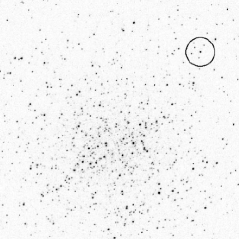
Figure 15: PC image of the Globular Cluster NGC 6440 cropped and displayed as a negative. The image scale is 0.046 ″/pixel. The black circle indicates the SIM FOV of 3″.

Most of the bright stars in this picture are K giants; we generated a catalog of these stars using the ‘SExtractor’ software. Although it is well known that this approach does not provide accurate photometry in crowded fields, our goal here is not to obtain precise corrections to the astrometric observations (which would require micro arc-second positions as well as accurate magnitudes) but rather to elucidate the general level and nature of the biases which may be expected. The number of sources which can be obtained with this software depends on the assumed value of the background intensity; after a few trials, we settled on a background value of $1.5\times\sigma_{rms}$, which yielded about 2400 stars with positions and V magnitudes. A visual comparison of the selected objects with the original image showed a good correspondence. The area density of these stars as a function of the radial distance from the center of the cluster is shown in Figure 16.

Figure 16: Number density of stars as a function of radial distance from the core of the cluster NGC 6440. The magnitudes of the stars lie in the range from 16.19 to 25.52

We then selected 51 circular fields at different locations in the cluster (one is shown in Figure 15); each field is centered on a bright star (presumed to be a K-giant). The model constructed for that field consists of a list of the positions and magnitudes of the target star and all field stars within a radius of 3″ of the target; this allows for diffraction of light into the 3″ (diameter) SIM FOV from stars which are located beyond the edge of the aperture.

The SEDs of the model stars were determined from estimates of surface temperature, gravity, and metallicity, as follows. From the V magnitudes (with the assumption that all stars are K giants) we attributed a temperature to a star randomly in the range 4000-4750 K (4000, 4250, 4500,4750) and a surface gravity randomly in the range of 1.5 to 4 with a step size of 0.5. We assumed that all the stars have solar metallicity. The spectra so determined were renormalized to account for the distance to the cluster and the magnitude of the field star.

5.4.2 Results

Figure 17: Probability that the confusion bias exceeds 10 $\mu{\rm as}$ in a single measurement as a function of radius of the globular cluster NGC6440.

In each of the 51 fields we obtained the confusion bias for 18 different orientations (position angles) of the SIM baseline (0° to 170° in steps of 10°). The fields used in this set of simulations typically have target stars at V $\approx$ 16-18, with brightest field stars at V $\approx 16$ or fainter, down to $\approx$ 25 (with some exceptional cases; in 5 out of 51 fields, brightest field stars were brighter than the target by 1.2, 1.6, 3.2, 2, 4.6 magnitudes; 3 of them were within the core radius and the remaining two were within 16 arcsec radius.). Of all the cases we analyzed in each field, 20% of them showed biases in excess of 10 $\mu{\rm as}$ in all 18 baseline orientations considered; Figure 17 shows the probability of a single measurement confusion bias exceeding 10 $\mu{\rm as}$ as a function of radius of the cluster. For a given field, if the confusion bias was more than 10 $\mu{\rm as}$ in 12 out of 18 orientations, the probability was estimated as 2/3 at the radial distance of the field from the center of the globular cluster. This figure indicates that, for NGC6440, the probability of having large confusion bias can be as large as 95% even at the radius of 15″ and there could be as much as 40% probability of large confusion bias at large radial distances. The probability of obtaining large confusion bias drops at larger radial distances in the cluster, as the local stellar surface density decreases. This latter point is illustrated in Figure 18, which shows the confusion bias as a function of baseline orientation for two different fields, located at radial distances of 3.6″ and 20″ from cluster center. For the field at 3.6″ (which is actually inside the cluster core), the biases are always large (note the logarithmic scale) at all baseline orientations. For the field at 20″, the error is larger than 10 $\mu{\rm as}$ in 30% of the baseline orientations.

Figure 18: Confusion bias as a function of baseline orientation for model fields located at 3.6″ (top panel) and 20″ (bottom panel) from the center of NGC 6440. Target fields at the periphery of clusters are clearly preferable, but may still have an appreciable probability (here $\approx 30\%$) for a substantial confusion bias.

5.4.3 Discussion

The statistics of these results indicate that the probability of having an unacceptable level ($\geq$ 10 $\mu{\rm as}$) of confusion bias in the positions of target stars is will exceed 30% for a single observation carried out at any random baseline orientation if the stellar density in the area exceeds 0.4 stars per square arc-second (compare Figures 16 and  17; In other words, about 3 stars within the 3″ FOV is acceptable).

However, the focus of this particular Key Project is on distances to objects, and hence on the parallaxes of the target stars. How do our results apply to the measurement of parallaxes? Such a measurement could be carried out with SIM in a special way, namely, ensuring that the baseline orientation was identical for observations taken $\approx 6$ months apart in time. This is perhaps possible in principle, but very unlikely in practice. First, the baseline orientation can not easily be set to $\approx 1$°; indeed, it is in fact generally not even known until the baseline vector has been calibrated. This means that parallaxes will suffer from the same magnitude of confusion bias as do regular position measurements. In the case of the cluster Key Project, a possible strategy could be to choose a number of target stars each at some large distance from the cluster center (such that the stellar density is lower than the limit cited above), and obtain parallaxes on each of them using the standard SIM observing strategy. Discordant single-measurement data points would then simply be rejected from the data set as a likely consequence of confusion.

6 Limitations of the models

The first, and perhaps most painful, limitation of the modeling we have described here is that, in spite of our apparent ability to compute the confusion bias in any single measurement with high precision, the results are in general not likely to be sufficiently accurate to provide actual corrections to the target positions. The simple reason for this is that the true field star positions are not known with accuracies of the same order as the expected single-measurement precision of SIM, $\approx 10$ $\mu{\rm as}$. Whether the modeling might be sufficient in any particular case will depend on the specific details of that field on the sky; our modeling tools (described in the next section) can then be used to evaluate the biases by e.g. varying the positions and brightnesses of the field stars over plausible ranges.

The second limitation of our modeling concerns the instrument model we have adopted for SIM. There are several simplifications we have made which could be problematic:

1. In our numerical simulations, we have assumed that the FOV is exactly circular, and that all the photons diffracted into it will be collected (with some efficiency) by the detector. However, in practice the focal plane of SIM’s camera will be covered by a CCD detector with pixels of $\approx 2$″ on a side, and it is presently planned to average the data in three neighboring rows.

2. We have assumed that the photons collected in each FOV will be dispersed in the camera in some way into 80 channels with central wavelengths and bandwidths as specified in Appendix B.1. In fact, a thin prism will be inserted into the light path before imaging onto the CCD detector, turning the camera into an objective prism spectrograph. Such instruments require special calibration and are subject to a degree of internal confusion caused by overlap of spectra from field stars with the spectrum of the target star.

3. We have estimated the fringe parameters (total power, fringe amplitude and fringe phase) analytically, and neglected the details of just how they will be measured on-board the spacecraft.

4. We have assumed that the throughput of the system is the same for different locations in the FOV. In fact, the presence of the prism will cause the throughput (and the dispersion) to change depending upon the angle of incidence at the prism, and hence to be different for the target and for the field stars.

We have carried out a further study using a more sophisticated instrument model which removes the first three of these limitations. The details of this extended model will be described elsewhere (Sridharan & Allen, 2007b), but we give here the results of repeating the bias computations on a subset of the fields we have described in the present paper. Table 1 compares the biases obtained using the “simplified” approach presented in this paper with those obtained using the more detailed model of the focal plane. The cases listed are taken from the Quasar Frame Tie key project (cases 1 - 5) and a selection of binary models (cases 6 - 8). Perhaps not surprisingly, the differences are roughly proportional to the magnitude of the computed bias, although these differences are generally at a level of only a few percent. Unfortunately, the utility of the results from this more sophisticated instrument model is still compromised by inaccurate input data on the field stars, and since it also comes with considerable additional complexity we have not used it further in this paper.

Table 1: Comparison of the single-measurement confusion bias obtained with the present simplified model and with the more detailed model of Sridharan & Allen (2007b).

Case	Model	Simple	Detailed	Difference
Number	parameters	($\mu{\rm as}$)	($\mu{\rm as}$)	($\mu{\rm as}$)
1	Q(z=0), A1V, 2, 50, 5, 90	0442	0431	11
2	Q(z=0), M6V, 2, 50, 5, 90	1072	1036	36
3	Q(z=2), A1V, 2, 50, 5, 90	0224	0215	09
4	Q(z=2), M6V, 2, 50, 5, 90	0614	0592	22
5	Q(z=2), M6V, 2, 50, 5, 10	0$-46$	0$-46$	00
6	A1V, B1V, 3, 1500, 10, 90	00$-1$	0000	01
7	A1V, M6V, 2, 50, 90, 90	0$-59$	0$-61$	02
8	A1V, M6V, 2, 25, 90, 90	0$-53$	0$-46$	07

Note. — In column 2, Q(z=0), A1V, 2, 50, 5, 90 means target quasar with redshift 2, A1V field star, $\Delta$m = 2, radial distance 50 mas, PA = 5°, baseline orientation 90°.

7 Modeling Tools

The source and instrument models described here have been implemented in a suite of programs written in the IDL programming system. These programs are available for further experimentation, including the code developed for estimating confusion bias in the specific target fields described in this paper.

8 Summary and Discussions

We have examined the bias that can occur in a single measurement with SIM owing to the presence of field stars within the FOV. In order to accomplish this task we have presented a model for the SIM interferometer, and a description of how SIM carries out a single measurement of the position of an isolated target star. The measured instrument response is then perturbed by adding a field star to the model FOV; the difference in the angles measured in the two cases is called the “confusion bias”. The extremes of this bias are calculated for the specific (but common) case of a binary system in order to illustrate its main properties.

A number of source models are then developed which resemble the fields to be studied by SIM in several of the Key Projects already selected for inclusion in the initial mission science program. An unconfused version of the source model consisting only of the main target star is used as a reference measurement, and the results compared with a measurement made on the fully-populated field. The difference is the confusion bias in a single SIM measurement. Observations are simulated at various orientations of the interferometer baseline, and variants of the full field are examined in order to understand the sensitivity of the bias to structural details in the field.

The magnitude of the confusion bias is found to depend on a number of factors, some obvious, others perhaps less so:

• the relative brightnesses of the target and the field stars;

• the shapes of the SEDs of the target and field stars;

• the angular separation of the stars from the center of the FOV;

• the angular separation of the field stars from the target star as projected on the interferometer baseline; and,

• the baseline orientation.

The largest contributions to the confusion bias in a crowded field come from a small number of stars having small projected angular separations from the target, but these stars may actually be located outside of the FOV. Field stars which are less than 4 mag fainter than the target and which have projected separations within 100 mas of the target are potentially the most troublesome.

The results of this study provides the understanding and the tools required to examine the likelihood of confusion bias in any single measurement with SIM. Unfortunately, data on the field stars in any specific FOV (especially their positions) is not likely to be available with sufficient accuracy to actually remove this bias. Our study nevertheless suggests some strategies for recognizing the presence of confusion bias and for dealing with it, both in the observation planning stage and in the data reduction stage. These strategies might include the following:

• While dealing with crowded fields, avoid fields with star densities in excess of 0.4 stars per square arcsec.

• If avoidance is impossible, evaluate the likelihood of confusion in the field by using the tools developed here.

• If confusion is likely, try to reduce your sensitivity to it by planning the observing program so that data is taken at the least sensitive orientations of the interferometer baseline.

• If too little is known about the specific field, plan to distribute the available observing time over a number of orientations of the interferometer baseline which differ by a few degrees from each other. Inconsistent values in the data set can then be rejected with motivation.

• If confusion is suspected in a given set of observations for which no prior data exists, acquiring new imagery from e.g., speckle or adaptive optics imaging would be useful for building a model.

There is one additional strategy suggested by our more accurate model of the SIM focal plane. The CCD detector in the focal plane of SIM’s camera is planned to have pixels which are smaller than the diameter of the FOV. If the data in the individual pixels can be made available, it would be possible to choose e.g. only the central pixel, thereby effectively reducing the FOV and possibly attenuating an offending field star. The penalty of fewer target photons could then be offset by a reduction in the level of confusion bias. This possibility will be discussed in more detail in a future paper (Sridharan & Allen, 2007b).

We wish to emphasize that the results of this paper refer to a bias which may be present in a single measurement of angular position with SIM. The determination of the full set of astrometric parameters (position, parallax, proper motion) on any SIM target will be done with a number of measurements, reducing the effects of any single anomalous point. Furthermore, the ultimate accuracy of the results depends on an extensive calibration program to determine the instrumental parameters, including the baseline length and orientations for each field observed.

Appendix A Michelson interferometer response

Michelson interferometers are used in astronomy at wavelengths from the radio to the optical for spectroscopy, for astrometry, and for synthetic imaging. The major equations giving the response of such interferometers for the latter two applications are summarized here.

A.1 Interferometers for astrometry and imaging

At any given wavelength $\lambda$ and baseline separation $B_{ij}$ (both e.g. in meters), the response of a simple adding Michelson interferometer of the type used for astrometry and imaging of partially coherent light in optical astronomy can be modeled as (e.g. Born & Wolf (1975), p. 491 et. seq.):

$$P(\Delta_{ij},k)=P_{0}[1+A\cos(2\pi k\Delta_{ij})],$$ (A1)

where $P_{0}$ is proportional to the target brightness (e.g. in photons/sec), $A\leq 1$ is called the fringe amplitude and depends on the target structure, $k=1/\lambda$ is the wavenumber (in e.g. meters^-1), and $\Delta_{ij}$ is the total optical path difference OPD (e.g. in meters) between the two sides (or “arms”) of the interferometer. For point source targets, $A=1$, and the normalized version of equation A1 can be considered as the interferometer’s far-field “point spread function” (PSF), similar in concept to the PSF of a filled-aperture telescope.

The total OPD $\Delta_{ij}$ consists of components on each side $i$ and $j$ of the interferometer, and each of those consists of an internal and an external part. Furthermore, some of the internal delay is “fixed”, and some may be “variable”. Referring to Figure 19 we can write:

$$\Delta_{ij} = [\mbox{total side $j$ delay}]-[\mbox{total side $i$ delay}],$$

where the components on each side are:

$\begin{array}[]{rcl}\mbox{side $j$ internal delay}&=&\mbox{fixed delay + variable delay}\\ &=&d_{j}+\delta,\mbox{ and}\\ \mbox{side $j$ external delay}&=&0\mbox{ by construction. Further,}\\ \mbox{side $i$ internal delay}&=&\mbox{fixed delay + variable delay}\\ &=&d_{i}+0\mbox{ by construction, and}\\ \mbox{side $i$ external delay}&=&B_{ij}\sin\theta.\end{array}$

This last equation is simple geometry, as Figure 19 shows, but it is often stated as the dot product of a vector B parallel to the direction of the baseline with a (unit) vector D in the direction for which we wish to compute $\Delta_{ij}$. D makes an angle of $\alpha$ with B, see Figure 19. Then the “side $i$ external delay” can be written as B $\bullet$ D $=B_{ij}\cos\alpha$. Defining $\alpha=\theta+\pi/2$ we have “side $i$ external delay” $=B_{ij}\sin\theta$, with $\theta$ defined as shown in Figure 19; in fact, $\theta$ is the half-opening angle of a cone with axis parallel to the interferometer baseline. Note that $\theta$ is also the angular distance of the direction of interest from a direction perpendicular to the baseline ($-\pi/2\leq\theta\leq+\pi/2$). Our idealized interferometer has a constant response in directions orthogonal to the baseline; the actual field of view will be further restricted by the practicalities of its design. Note further that equation A1 also closely describes the pattern in transmission, such as would occur if a laser (or CW radio transmitter) would be sent from an appropriate point in the beam path backwards through the interferometer. This is an expression of a general reciprocity theorem, familiar in radio engineering, which is itself rooted in the symmetry of the wave equation for the electromagnetic field with respect to the direction of time.

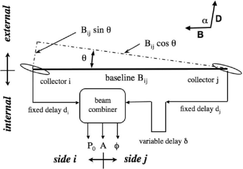
Figure 19: Sketch of the basic Michelson interferometer as used for astrometry and imaging in radio and optical astronomy. B is a vector in the direction of the baseline, and D a unit vector in the direction in which we want to compute the interferometer’s response. $\theta=\alpha-\pi/2$, and P₀, A, and $\phi$ are defined in the text.

Finally, equation A1 applies only at a single wavelength; one must also account for the finite bandpass. In essence the response becomes a sum of many different patterns within the bandpass, and the coefficient of the “cos” term in equation A1 will be multiplied by a factor which is essentially the Fourier Transform of the band shape for that specific channel. Without detailed knowledge of that band shape we can not calculate the final form of equation A1; however, the results are likely to be amenable to a simple parameterization, using the following definitions. The mean wavenumber $\overline{k_{n}}$ for channel $n$ is defined as:

$$\overline{k_{n}}=\frac{\int kF_{n}(k)dk}{\int F_{n}(k)dk},$$ (A2)

where $F_{n}(k)$ is the band shape of channel $n$ expressed in wave numbers ($k=1/\lambda=\nu/c$, where $\nu$ is the frequency in Hz). The coherence length $\Lambda_{n}$ (e.g. in meters) for channel $n$ is defined here as:

$$\Lambda_{n}\approx 1/(\Delta k)_{n}$$ (A3)

where $(\Delta k)_{n}$ is the full width at half maximum of an assumed Gaussian band shape $F_{n}(k)$ centered at $\overline{k_{n}}$. The coherence length is the scale size of the wave packet formed by the collection of photons at various neighboring wave numbers that make up the broad-band signal. It is given by the expression $\Lambda_{n}=\overline{\lambda}^{2}/\overline{\Delta\lambda}$. With these definitions we can write our model expression for the fringe pattern in channel $n$ as:

$$P(\Delta_{ij},\overline{k_{n}},\Lambda_{n})=P_{0}\{1+Ae^{-C\left(\frac{\Delta_{ij}}{\Lambda_{n}}\right)^{2}}\cos(2\pi\overline{k_{n}}\Delta_{ij})\}$$ (A4)

where $C=\pi^{2}/4\ln 2=3.56$. Suppose further that we design the interferometer such that $d_{i}=d_{j}$ (or define $\delta=0$ such that this occurs), then the OPD becomes:

$$\Delta_{ij}=\delta-B_{ij}\sin\theta.$$ (A5)

Inserting this last relation into equation A4 gives the final (approximate) expression for the interferometer response in a single channel of finite bandwidth:

$$P(\delta,\theta,\overline{k_{n}})=P_{0}\{1+Ae^{-3.56\left[\frac{\delta-B_{ij}\sin\theta}{\Lambda_{n}}\right]^{2}}\cos(2\pi\overline{k_{n}}[\delta-B_{ij}\sin\theta])\}.$$ (A6)

Considered as a function of $\theta$ this equation describes the fringe pattern anywhere in the sky for a given value of internal delay $\delta$. Alternatively, equation A6 describes the response to a source located at a fixed $\theta$ in the sky as a function of the internal delay $\delta$.

Equation A6 needs to be modified in order to render it specific to SIM. First, SIM’s optical beam combiner effectively adds an additional $\pi/2$ of phase delay to one of the incoming beams, turning the “cosine” function into a “sine”. Second, SIM always “observes” in a direction closely perpendicular to the baseline orientation (cf. Figure 19), so that $\theta$ is small and we can set $\sin\theta\approx\theta$. Third, the exponential term describing the amplitude decorrelation can be set to unity, as the bandwidths of the individual channels are narrow. With these changes, and ignoring the subscripts $ij$ of the baseline $B$, we can write equation A6 for any channel with mean wavenumber $\overline{k}$ as:

$$P(\delta,\theta,\overline{k})=P_{0}\{1+A\sin(2\pi\overline{k}[\delta-B\theta])\}.$$ (A7)

Appendix B Instrument and Model Details

B.1 Current SIM parameters

Our SIM instrument model assumes the following values for the various parameters required in the simulation of the interferometer response:

Baseline length: 9.000 m for the astrometric interferometer.

Collector size: Siderostats, outer diameter 304.5 mm, inner diameter 178 mm, net area = 479.378 cm².

Field stop size: Nominally 3″ diameter. However, this can be chosen in the simulation code to be any one of four possible values (1,2,3 or 4″).

Number of channels and bandwidth: The design for the fringe disperser in SIM has 80 narrow-band channels with bandwidths progressively increasing from 1.8 nm at 401.9 nm, to 24.9 nm at 985.5 nm. The band shape is likely to be approximately Gaussian, and this is what we have used; however, the simulation code allows the user to choose a rectangular passband instead. The list of central wavelengths and bandwidths assumed for these simulations can be found at the author’s web site.

Throughput ($Th$): The Throughput varies across the 80 channels, depending on the reflection/transmission optics and the QE and spectral response of the detector. We found that the experimentally-measured values could be modeled best using the relation $Th=\sum_{i=0}^{7}c_{i}\lambda^{i}$ with $c_{0}=18.2$, $c_{1}=-338.5$, $c_{2}=2076.2$, $c_{3}=-6239.4$, $c_{4}=10463.3$, $c_{5}=-10029.1$, $c_{6}=5151.4$ and $c_{7}=-1102.1$, for $\lambda$ expressed in microns.

Pointing accuracy: There are two parts to the “pointing” of SIM: The angle tracker will center the target in the instrument FOV and superpose the images from each side of the interferometer to within 10 mas for bright targets $V_{target}<15$, and 30 mas for faint targets $15<V_{target}<19$. The fringe tracker will set the coarse delay on the target with an accuracy of 10 nm (for $V_{target}<10$, corresponding to a maximum offset of $\approx 0.2$ mas at 500 nm.

Spectral dispersion: A thin prism is inserted into the light path after beam combination, turning the instrument into an objective prism spectrograph, such that the images of stars in the focal plane are stretched out into spectra in a direction approximately parallel to the projection of the SIM baseline on the sky. For a target at the center of the FOV, the experimentally-measured dispersion can be modeled with the polynomial $x=\sum_{i=0}^{6}c_{j}\nu^{j}$ with $c_{0}=5.1$, $c_{1}=-2.7$, $c_{2}=1.0$, $c_{3}=-0.23$, $c_{4}=0.03$, $c_{5}=0.002$, and $c_{6}=0.00005$, for $\nu$ in units of 10¹⁴Hz and $x$ in mm.

Focal plane camera: The camera has pixels of size 24 $\mu$ aligned along the direction of dispersion; however, we ignore the pixellation of the focal plane camera in the simulations described in this paper.

Overall measurement precision: The design goal is to make a single measurement of the angular position of a target on the sky with a precision of $\lesssim 10$ $\mu{\rm as}$. As the fringe period $\lambda/B$ is typically 10 - 20 mas and the baseline length is about $10-20\times 10^{6}\lambda$, the design requirement on the single-measurement angular precision corresponds to $\approx 1/1000$ of a fringe.

B.2 Estimation of Total Power

In this Appendix we present the mathematical details of how we estimated the total light from the target and field stars that lie within and just outside the 3″ FOV of SIM.

Figure 20: Fraction of the energy recorded for a star located at a given radial distance from the center of the (circular) FOV of SIM, for field stops of 2, 3 and 4″ diameter, and at several different wavelengths.

For the target star, the total energy received by the interferometer in each channel is multiplied by the throughput and the encircled energy within the aperture at the mean wavelength $\bar{\lambda}$ (to account for the FOV set by the field-stop) and integrated over the bandpass to obtain the total power in that channel. It is then multiplied by $hc/{\bar{\lambda}}$ to obtain the number of photons/second/channel.

In the case of the field stars, the total energy is obtained as follows: Consider a Cartesian coordinate system centered on the target star which is also at the center of the FOV. Suppose that there is a field star at ($x_{0},y_{0}$). The energy of that part of the diffracted image that lies within the field stop is obtained by calculating the integral of the product of the point spread function (PSF) centered at ($x_{0},y_{0}$) and a pill-box function representing the field-stop. This is equivalent to integrating the product of the on-axis PSF representing the field star with a shifted version of the pill-box function centered at ($x_{0},y_{0}$). The expression is:

$$EF_{bg\star}(x_{0},y_{0})=\int\int PSF(x,y)\times\mbox{Circ}(x-x_{0},y-y_{0})dxdy$$ (B1)

where the “Circ” function is defined as:

$$\mbox{Circ($x,y$)}=\left\{\begin{array}[]{ll}1&\mbox{if $x^{2}+y^{2}<(FSD/2)^{2}$}\\ 0&\mbox{otherwise,}\end{array}\right.$$

and $EF$ is the estimated flux, PSF is the point spread function, and FSD is the field stop diameter. From this representation it is clear that the energy of the field star that lies within the field stop is the convolution (or correlation) of the on-axis PSF of the field star with a pill-box function located at ($x_{0},y_{0}$). It is convenient to normalize this correlation function and obtain a fractional number which, when multiplied by the total energy received by the interferometer from the field star, provides the desired value. This value is further multiplied by the throughput of the system and converted into photons/second/channel for each field star. Figure 20 shows this overall transmission function for several possible field stop sizes and wavelengths. We have computed this response function at the mean wavelength of each channel.

References

- Boden (2004) Boden, A. 2004, “Space Interferometry Mission, Data Product Document,” Jet Propulsion Laboratory & Michelson Science Center, Caltech, Pasadena, California.
- Born & Wolf (1975) Born, M., & Wolf, E. 1975, “Principles of Optics,” (Oxford, Pergamon)
- Dalal & Griest (2001) Dalal, N., & Griest, K. 2001, ApJ, 561, 481
- Gaskill (1978) Gaskill, J.D. 1978, “Linear Systems, Fourier Transforms, and Optics” (New York, Wiley), Section 2-2
- Hecht (2002) Hecht, E. 2002, “Optics” (Addison Wisely)
- Milman & Basinger (2002) Milman, M. H., & Basinger, S. 2002, Appl. Opt., 41, 2655.
- Milman & Turyshev (2003) Milman, M. H., & Truyshev, S. V. 2003, Opt. Eng., 42, 1873.
- Philips (1961) Phillips, E.G. 1961, “Functions of a Complex Variable” 8th ed. (Edinburgh, Oliver & Boyd), 5
- Rajagopal et al. (2001) Rajagopal, J., Böker, T., & Allen, R.J. 2001, PASP, 113, 1232
- Sridharan & Allen (2007b) Sridharan, R. & Allen, R. J., 2007b, in preparation
- Takeuchi et al. (2005) Takeuchi, T., Velusamy, T., & Lin, D. N. C. 2005, ApJ, 618, 987
- White et al. (2000) White, R.L., Becker, R.H., Gregg, M.D., Laurent, M.S.A (& and 11 co-authors) 2000, ApJS, 126, 133