Expansions for the Bollobás-Riordan polynomial of separable ribbon graphs

Abstract.

We define 2-decompositions of ribbon graphs, which generalise 2-sums and tensor products of graphs. We give formulae for the Bollobás-Riordan polynomial of such a 2-decomposition, and derive the classical Brylawski formula for the Tutte polynomial of a tensor product as a (very) special case. This study was initially motivated from knot theory, and we include an application of our formulae to mutation in knot diagrams.

1. Introduction

We are interested in the decomposition of graphs and ribbon graphs into their 2-connected components. Suppose a graph $\widehat{G}$ is 2-separable. We may regard it as arising from the 2-sums of a collection of graphs $\left\{{A}_{e}\right\}_{e\in E}$ with the graph $G=(V,E)$. Here the subscript $e$ plays two roles: it labels the individual graphs in the collection $\left\{{A}_{e}\right\}_{e\in E}$, and within each of these graphs it distinguishes the edge along which the two-sum is to be taken. The graph $G$ determines how the graphs $\left\{{A}_{e}\right\}_{e\in E}$ are assembled. Strictly speaking, the 2-sum is not well-defined on graphs without specifying which way round the edges are to be identified: in what follows we overcome that by referring to the vertices $u_{e}$ and $w_{e}$ at each end of the edge $e$. Also, it will often be more convenient for us to work with the graphs $H_{e}=A_{e}\setminus\{e\}$. We will call the structure $\left(G,\{H_{e}\}_{e\in E}\right)$ a 2-decomposition for $\widehat{G}$. There are two important special cases. One arises when $G$ is the graph on two vertices with two edges $e,f$ joining them. Then $\widehat{G}$ is the conventional two-sum $A_{e}\oplus_{2}A_{f}$. The other arises when all of the $A_{e}$ are equal to a graph $A$. Then $\widehat{G}$ is the tensor product $G\otimes A$ [18].

It is natural to seek the connection between the graph polynomials of $\widehat{G}$ and those of $G$ and the $H_{e}$. There is a well known result due to Brylawski [4] which describes the Tutte polynomial of the tensor product $T(G\otimes A)$ in terms of those of its two factors $G$ and $A$. This result has played an important role in the complexity theory of the Tutte polynomial [9, 13, 14]. Brylawski’s result also plays a role in knot theory: in [11] the first author used Brylawski’s result to explore the relation between the realizations of the Jones and HOMFLY polynomials as evaluations of the Tutte polynomial of an associated graph [1, 12, 14, 21].

Another recent example of the connection between the polynomials of $\widehat{G}$ and those of its 2-decomposition comes from Woodall [22]. In this paper he expressed the Tutte polynomial of $\widehat{G}$ in terms of the graphs $H_{e}$ and either the flow polynomials of subgraphs of $G$ or the tension polynomials of contractions of $G$. This work is related to problems on the homeomorphism classes of graphs.

Here we are interested in generalizing the results of Brylawski in two directions. We want to drop the condition that all of the graphs $H_{e}$ are equal, and we also want to generalize the formula to ribbon graphs (graphs with a cyclic ordering of each of the incident half-edges at each vertex). This latter will entail the study of the Bollobás-Riordan polynomial, which is the generalization of the Tutte polynomial to ribbon graphs.

Brylawski’s proof of the tensor product formula uses the universal properties of the Tutte polynomial. This approach, however, only works for the tensor product and cannot be extended to our 2-decompositions of graphs (although we acknowledge that Brylawski’s proof does have the advantage that it can be extended to matroids). Moreover, the universal properties of the Bollobás-Riordan polynomial do not seem to be strong enough to support this method of proof of a Brylawski theorem for ribbon graphs (because the basis would consist of all 1-vertex ribbon graphs). Thus we see that a new approach is needed.

The idea behind our approach is simple. The Bollobás-Riordan and Tutte polynomials can be described as a sum over states, where a state is a spanning (ribbon) subgraph. The polynomials count the number of edges, connected components and, for the Bollobás-Riordan polynomial, the number of boundary cycles of the states. Let $\widehat{G}$ be as above. There is an obvious bijection between the states of $\widehat{G}$ and states of $\cup_{e\in E}H_{e}$. This gives a decomposition of the states of $\widehat{G}$. We are interested in calculating the Bollobás-Riordan and Tutte polynomials, so we also need a way of relating the number of connected components and boundary cycles in the states of $H_{e}$ to those in the corresponding state of $\widehat{G}$. The ribbon graph $G$ describes how each of the copies of $H_{e}$ are linked together to form $\widehat{G}$, and we use the states of $G$ to relate the states of $\widehat{G}$ and $\cup_{e\in E}H_{e}$.

Here is a brief plan of the paper. Section 2 defines ribbon graphs and their polynomials. In Section 3 we show how to calculate the Tutte polynomial of $\widehat{G}$ in terms of its 2-decomposition, generalizing the result of Brylawski. We extend our methods to ribbon graphs and the Bollobás-Riordan polynomial in Section 4 and show that in special cases we can calculate the Bollobás-Riordan polynomial of a ribbon graph from its 2-decomposition. In Section 5 we show how the Bollobás-Riordan polynomial of any ribbon graph can be calculated from its 2-separation by considering geometric ribbon graphs. We give applications of our results to the construction of ribbon graphs with the same polynomials, and we finish in Section 6 with an application of our work to the study of mutations in knot diagrams.

I.M. would like to thank Anna De Mier for helpful conversations on the Tutte polynomial. We are very grateful for the referee’s careful reading and helpful comments.

2. Preliminaries

2.1. Ribbon graphs and 2-decompositions

A ribbon graph $G=(V,E)$ is an orientable surface with boundary represented as the union of $V$ closed disks and $E$ ribbons, $I\times I$, ($I=[0,1]$ is the unit interval) such that

1. the discs and ribbons intersect in disjoint the line segments $\{0,1\}\times I$;

2. each such line segment lies on the boundary of precisely one disk and precisely one ribbon;

3. every ribbon contains exactly two such line segments.

Ribbon graphs arise naturally as neighbourhoods of graphs embedded in orientable surfaces. In fact it is well known that ribbon graphs are equivalent to cellularly embedded graphs in an orientable surface (for example, see [10]). Any such embedding, together with a choice of orientation of the surface, induces a cyclic ordering of the incident half-edges at each vertex of the graph. Thus an oriented ribbon graph is equivalent to a graph (possibly with multiple edges and loops) with a fixed cyclic ordering of the incident half-edges at each of its vertices. We will find the latter purely combinatorial description useful on occasion.

Recall that a graph is said to be n-separable if there exists a set of $n$ vertices whose removal disconnects the graph. $n$-separability is a fundamental property of the structure of a graph. By itself, this decomposition of graphs is too coarse for ribbon graphs as it ignores the cyclic order at the vertices and therefore the inherent topology. For example, the graph with one vertex and two edges $e$ and $f$ is clearly 1-separable. However, the two choices of cyclic order of the half-edges $e,e,f,f$ and $e,f,e,f$ give rise to two distinct ribbon graphs with very different properties, which are not captured by their 1-separable components.

However, the notion of a 2-sum is more subtle: given two graphs $G$ and $F$ with distinguished edges $e\in E(G)$ and $f\in E(F)$, the 2-sum $G\oplus_{2}F$ is defined by identifying $e$ with $f$ (making a choice of which way round to do this) and then deleting the identified edge. This works just as well when $G$ and $F$ are ribbon graphs: in the process of identifying $e$ with $f$, suppose that the vertex $u_{e}\in V(G)$ is identified with $u_{f}\in V(F)$. We choose orientations for these ribbon graphs, and suppose further that $e$ and $f$ are not loops and the cyclic orders around these two vertices were $\{e,e_{1},\dots,e_{n}\}$ and $\{f,f_{1},\dots,f_{m}\}$. Once the identified edge has been deleted, the cyclic order around the new vertex will be $\{e_{1},\dots,e_{n},f_{1},\dots,f_{m}\}$. This is illustrated in figure 1. In the case when $e$ is a loop and $f$ is not we suppose that $u_{e}$ has cyclic ordering $\{e,e_{1},\dots,e_{k},e,e_{k+1},e_{n}\}$ and the vertices $u_{f}$ and $w_{f}$ of the edge $f=(u_{f},w_{f})$ have cyclic orderings $\{f,f^{1}_{1},\dots,f^{1}_{m}\}$ and $\{f,f^{2}_{1},\dots,f^{2}_{l}\}$ respectively. Then once the identified edge has been deleted, the cyclic order around the new vertex will be $\{e_{1},\dots,e_{k},f^{1}_{1},\dots,f^{1}_{m},e_{k+1},\dots,e_{n},f^{2}_{1},\dots,f^{2}_{l}\}$. This is illustrated in figure 2.

We would like to emphasise the fact that in the formation of the 2-sum we arbitrarily assigned orientations to the the two summands and that the 2-sum is an orientation preserving operation. In general, the resulting ribbon graph will depend upon the choice of orientations used in the formation of the 2-sum.

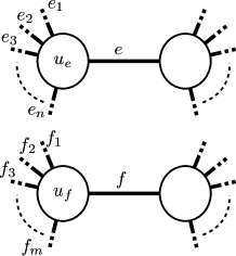
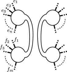
   $$\longrightarrow \longrightarrow$$         

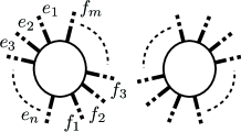
Figure 1.

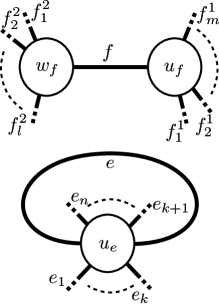
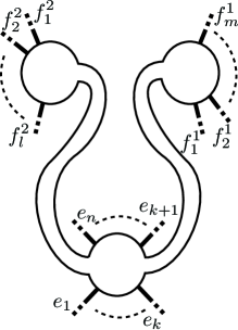
   $$\longrightarrow \longrightarrow$$         

Figure 2.

Definition 1.

Let $G=(V,E)$ be a (ribbon) graph and $\left\{A_{e}\right\}_{e\in E}$ be a set of (ribbon) graphs each of which has a specific non-loop edge distinguished. For each $e\in E$ take the 2-sum $G\oplus_{2}A_{e}$, along the edge $e$ and the distinguished edge in $A_{e}$, to obtain the (ribbon) graph $\widehat{G}$. For each $e\in E$ define $H_{e}=A_{e}\setminus\{e\}$. We will call the structure $\left(G,\{H_{e}\}_{e\in E}\right)$ a 2-decomposition for $\widehat{G}$. The (ribbon) graph $G$ is called the template.

Examples of 2-decomposition are given in Figures 3, 4, and 8.

Note that each of the (ribbon) graphs $H_{e}$ has two distinguished vertices: those which were joined by the distinguished edge in $A_{e}$. We will denote these two distinguished vertices of each $H_{e}$ as $u_{e}$ and $w_{e}$ throughout this paper, and we will also use $u_{e}$ and $w_{e}$ to denote the vertices of the edge $e$ of $G$. We will assume (without loss of generality) that the vertices $u_{e}$ and $w_{e}$ of $H_{e}$ are distinct, but we make no such assumption on the vertices $u_{e}$ and $w_{e}$ of $G$, so $e$ may be a loop. This means that the 2-sum of ribbon graphs may be a 1-sum of graphs.

If each of the (ribbon) graphs $H_{e}$ in a $2$-decomposition are equal to a (ribbon) graph $H$, and if $u_{e}$ and $w_{e}$ lie in the same connected component, then $\widehat{G}$ is the tensor product of $G$ with $A$, written $\widehat{G}=G\otimes A$.

Finally, if $G=C_{2}$, the 2-cycle with edges $e$ and $f$, then $\widehat{G}$ is the 2-sum $A_{e}\oplus_{2}A_{f}$.

2.2. Tutte and Bollobás-Riordan polynomials

Again let $G=(V,E)$ be a (ribbon) graph. A state of $G$ is a spanning (ribbon) subgraph $(V,E^{\prime})$ where $E^{\prime}\subseteq E$. We denote the set of states by $\mathcal{S}(G)$. We will often abuse notation and write “state” when we mean “a subset $E^{\prime}\subset E$” and vice versa. In particular, we will often write “$e\in s$” rather than “$e\in E(s)$”. This abuse of notation should cause no confusion. If $s=(V,E^{\prime})\in\mathcal{S}(G)$ then we define $v(s):=|V|$, $e(s):=|E^{\prime}|$, $\neg e(E^{\prime}):=|E|-e(E^{\prime})$, $r(s):=|V|-k(s)$ and $n(s):=e(s)-r(s)$, where $k(s)$ denotes the number of connected components of $s$. Regarding a ribbon graph as a surface, we set $\partial(s):=|\partial(s)|$, the number of its boundary components. By a planar ribbon graph we mean one that can be regarded as a genus zero surface.

We are interested in expansions for the Tutte polynomial of a graph and the Bollobás-Riordan polynomial [2, 3], which is the natural generalization of the Tutte polynomial to ribbon (or embedded) graphs. The Bollobás-Riordan polynomial for ribbon graphs is defined as the sum

(1) $$R(G;\alpha,\beta,\gamma)=\sum_{s\in\mathcal{S}(G)}(\alpha-1)^{r(G)-r(s)}\beta^{n(s)}\gamma^{k(s)-\partial(s)+n(s)}.$$

For example,

$$R\left(\raisebox{-8.53581pt}{\psfig{height=22.76219pt}};\alpha,\beta,\gamma\right)=\beta^{2}\gamma^{2}+\alpha+2\beta+2.$$

Observe that when $\gamma=1$ this polynomial becomes the Tutte polynomial:

$$R(G;x,y-1,1)=T(G;x,y):=\sum_{s\in\mathcal{S}(G)}(x-1)^{r(G)-r(s)}(y-1)^{n(s)}.$$

This coincidence of polynomials also holds when the ribbon graph $G$ is planar. In fact the exponent of $\gamma$ is twice the genus of the state.

Before proceeding we also note that expanding the definitions of $r(s)$ and $n(s)$ in (1) yields the following equivalent form of the Bollobás-Riordan, and hence Tutte, polynomials:

(2) $$R(G;\alpha,\beta,\gamma)=(\alpha-1)^{-k(G)}(\beta\gamma)^{-v(G)}\sum_{s\in\mathcal{S}(G)}((\alpha-1)\beta\gamma^{2})^{k(s)}(\beta\gamma)^{e(s)}(\gamma)^{-\partial(s)}.$$

This rewriting of the polynomials is fundamental to our approach.

We need to consider multivariate generalizations of the Tutte and Bollobás-Riordan polynomials. (We will then specialize to the above polynomials where appropriate). The multivariate Tutte polynomial has been used extensively, and we refer the reader to Sokal’s survey article [19] for an exposition of its properties. The multivariate Bollobás-Riordan polynomial is the obvious extension of the multivariate Tutte polynomial. It has been used previously [6, 16, 17].

The multivariate Bollobás-Riordan polynomial of a ribbon graph $G=(V,E)$ is

(3) $$Z(G;a,{\bf x},c)=\sum_{s\in\mathcal{S}(G)}a^{k(s)}\left(\prod_{e\in s}x_{e}\right)c^{\partial(s)}\;\;\in\mathbb{Z}\left[a,\{x_{e}\}_{e\in E},c\right],$$

where ${\bf x}$ denotes the set $\{x_{e}\}_{e\in E}$. The multivariate Tutte polynomial ([19]) is then the specialization

(4) $$Z(G;a,{\bf x}):=Z(G;a,{\bf x},1)=\sum_{s\in\mathcal{S}(G)}a^{k(s)}\left(\prod_{e\in s}x_{e}\right).$$

When we set all of the variables $x_{e}$ equal to $b$, say, then we will denote the polynomial $Z(G;a,{\bf x},c)|_{x_{e}=b}$ simply by $Z(G;a,b,c)$. Notice that by equation (2),

(5) $$R(G;\alpha,\beta,\gamma)=(\alpha-1)^{-k(G)}(\beta\gamma)^{-v(G)}Z\left(G;(\alpha-1)\beta\gamma^{2},\,\beta\gamma,\,\gamma^{-1}\right),$$

so that the specialization is equivalent to the Bollobás-Riordan polynomial. A similar relation holds for (4) and the Tutte polynomial.

When the choice of variables is clear from the context we will just write $Z(G)$ instead of $Z(G;a,{\bf x},c)$ or its specializations (such as $x_{e}=b$ or $c=1$).

Notation 1.

Henceforth $\widehat{G}$ will always denote a (ribbon) graph with the 2-decomposition $\left(G,\{H_{e}\}_{e\in E}\right)$. Here $H_{e}$ denotes the graph $A_{e}$ with its distinguished edge (joining the vertices $u_{e}$ and $w_{e}$) deleted. We will often only need to pick out this distinguished edge in $Z(A_{e};a,{\bf x},c)$, so we denote by ${\bf b}$ the specialization of ${\bf x}$ which leaves $x_{e}$ as it is but for all $d\,(\neq e)\in E(A_{e})$ sets $x_{d}=b$. In a ribbon graph the distinguished edge will be between the marked points $m_{e}$ and $n_{e}$ described later in Subsection 4.1 and Figure 5.

2.3. Deletion and contraction for ribbon graphs

Later we will find it convenient to express our results in terms of the deletion and contraction of a ribbon in a ribbon graph. Here, we use the surface description of a ribbon graph. The deletion of a ribbon always makes sense, but we need to be more careful when we contract a ribbon.

Let $e$ be a ribbon of $F$. First suppose that $e$ is not a loop. Then $e$ is a ribbon between two distinct disks $u$ and $w$ of $F$. Suppose that the cyclic order of incident half-edges is $e_{u1},\ldots,e_{un},e$ at $u$, and $e,e_{w1},\ldots,e_{wn}$ at $w$. Then $F/e$ is the ribbon graph obtained by replacing the vertices $u$ and $v$ with a single vertex with cyclically ordered incident edges $e_{u1},\ldots,e_{un},e_{w1},\ldots,e_{wn}$.

Next suppose that $e$ is a loop. To describe the contraction of a loop we need a generalization of ribbon graphs, by allowing identifications of the boundary of any disk in a ribbon graph. We define a ribbon surface to be a surface with boundary represented as the union of $|V|$ closed surfaces with boundary, called nodes, and $|E|$ ribbons, $I\times I$, such that

1. the nodes and ribbons intersect in disjoint line segments $\{0,1\}\times I$;

2. each such line segment lies on the boundary of precisely one node and precisely one ribbon;

3. every ribbon contains exactly two such line segments.

The contraction of a loop $e$ is then defined by identifying the endpoints $\{0\}\times I$ and $\{1\}\times I$ of $e$ and then deleting $e$.

Note that if all of the nodes are disks, then an orientable ribbon surface is exactly a ribbon graph. We carry over all of our notation for ribbon graphs, except that by $v(F)$ we mean the number of nodes. With this inherited notation the Bollobás-Riordan polynomial of a ribbon surface makes sense. Moreover the following deletion-contraction relation now holds for any edge $e$:

(6) $$Z(F;a,{\bf x},c)=Z(F\backslash e;a,{\bf x},c)+x_{e}Z(F/e;a,{\bf x},c).$$

Notice that this generalizes the deletion-contraction relations for the Bollobás-Riordan polynomial given in [3] for ordinary edges and trivial loops.

We shall abuse notation and extend to ribbon surfaces without comment when the need arises. It is possible to avoid the generalization to ribbon surfaces, but it is much more convenient and concise to be able to use a deletion-contraction relation for loops.

2.4. Geometric ribbon graphs

A geometric ribbon graph is defined just as in the surface realization of a ribbon graph but without the condition of orientability, so we allow the ribbons between the disks to be twisted any number of times.

We carry over all of the notation for ribbon graphs, in particular that of Subsection 2.1, to geometric ribbon graphs. The one additional piece of information we need from a state of $F$ is whether it is orientable or not. Let $s\in\mathcal{S}(F)$; we set $t(s)=0$ if $s$ is orientable and $t(s)=1$ if $s$ is non-orientable.

The Bollobás-Riordan polynomial for geometric ribbon graphs (see [3]) is defined as follows.

$$R(F;\alpha,\beta,\gamma,\delta)=\sum_{s\in\mathcal{S}(F)}(\alpha-1)^{r(F)-r(s)}\beta^{n(s)}\gamma^{k(s)-\partial(s)+n(s)}\delta^{t(s)}\;\;\in\mathbb{Z}\left[\alpha,\beta,\gamma,\delta\right]/(\delta^{2}-\delta).$$

Observe that when $\delta=1$ or $F$ is orientable this polynomial coincides with the Bollobás-Riordan polynomial (1).

As with the ribbon graph polynomial, we need to use a multivariate version of this polynomial. The multivariate Bollobás-Riordan polynomial of a geometric ribbon graph $F=(V,E)$ is

$$Z(F;a,{\bf x},c,d)=\sum_{s\in\mathcal{S}(F)}a^{k(s)}\left(\prod_{e\in s}x_{e}\right)c^{\partial(s)}d^{t(s)}\;\;\in\mathbb{Z}\left[a,\{x_{e}\}_{e\in E},c,d\right]/(d^{2}-d),$$

where ${\bf x}$ denotes the set $\{x_{e}\}_{e\in E}$.

When we set all of the variables $x_{e}$ equal to $b$, say, then we will denote the polynomial by $Z(G;a,b,c,d)$. We then have

$$R(G;\alpha,\beta,\gamma,\delta)=(\alpha-1)^{-k(G)}(\beta\gamma)^{-v(G)}Z\left(G;(\alpha-1)\beta\gamma^{2},\,\beta\gamma,\,\gamma^{-1},\,\delta\right).$$

Remark 1.

Although we have favoured a surface description of geometric ribbon graphs here, everything could have been defined in terms of graphs with a fixed cyclic ordering of the incident half-edges at each vertex by adding a $+$ or $-$ sign on each edge to record the parity of the number of half-twists. We refer the reader to Bollobás and Riordan’s article [3] for details.

3. The Tutte polynomial

3.1. The Decomposition

Suppose we are given a state $\hat{s}\in\mathcal{S}(\widehat{G})$ and a 2-decomposition $\left(G,\{H_{e}\}_{e\in E}\right)$ of $\widehat{G}$. The state $\hat{s}$ is uniquely determined by a set of edges, but each of these edges also belongs to a graph in the set $\{H_{e}\}_{e\in E}$. Therefore the state $\hat{s}$ uniquely determines a set of states $\{s_{e}\in\mathcal{S}(H_{e})\}_{e\in E}$.

Now by the definition of 2-decomposition, each graph $H_{e}$ has two distinguished vertices $u_{e}$ and $w_{e}$ which are also vertices of $G$. For each $e$ we partition the states of $\mathcal{S}(H_{e})$ into two subsets: $\mathcal{S}^{1}(H_{e})$ consists of all states in $\mathcal{S}(H_{e})$ in which $u_{e}$ and $w_{e}$ lie in the same connected component, and $\mathcal{S}^{2}(H_{e})$ consists of all states in $\mathcal{S}(H_{e})$ in which $u_{e}$ and $w_{e}$ lie in different connected components.

We will use the partition of each set $\mathcal{S}(H_{e})$ to construct a state of $G$ from the states $\{s_{e}\}$ determined by $\hat{s}\in\mathcal{S}(\widehat{G})$ as above. To do this, start with the graph $G$ and then remove an edge $e=(u_{e},w_{e})$ if and only if the state $s_{e}$ determined by $\hat{s}$ lies in the set $\mathcal{S}^{2}(H_{e})$. An example is shown in Figure 3 where $\widehat{G}=C_{3}\otimes C_{3}$.

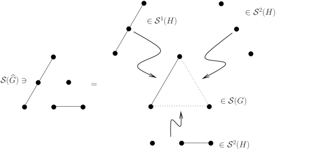
Figure 3.

If we replace the edges $e$ in a state $s\in\mathcal{S}(G)$ with elements of $\mathcal{S}^{1}(H_{e})$, and the edges $f$ which are not in $s$ by elements of $\mathcal{S}^{2}(H_{f})$, we obtain a state $\hat{s}\in\mathcal{S}(\widehat{G})$. Moreover, each state of $\widehat{G}$ is uniquely obtained in this way: we could start with $\hat{s}\in\mathcal{S}(\widehat{G})$ and from it determine an element of $\mathcal{S}^{1}(H_{e})\cup\mathcal{S}^{2}(H_{e})$ for each $e\in E$, and an element of $\mathcal{S}(G)$.

Lemma 1.

If a state $\hat{s}\in\widehat{G}$ is decomposed into states $s\in\mathcal{S}(G)$, $s_{e}\in\mathcal{S}^{1}(H_{e})\cup\mathcal{S}^{2}(H_{e})$, $e\in E$, then

$$k(\hat{s})=\sum_{e\in E}k(s_{e})-|\{s_{e}\in\mathcal{S}^{1}(H_{e})\}|-2|\{s_{e}\in\mathcal{S}^{2}(H_{e})\}|+k(s).$$

Proof.

Each component of $s$ corresponds to a component of $\hat{s}$, but $\hat{s}$ has extra components, arising from states $s_{e}\in\mathcal{S}^{1}(H_{e})\cup\mathcal{S}^{2}(H_{e})$ which have components not containing any vertices of $G$. For each $e\in E$ for which $s_{e}\in\mathcal{S}^{1}(H_{e})$ there are $k(s_{e})-1$ of these extra components, while if $s_{e}\in\mathcal{S}^{2}(H_{e})$ there are $k(s_{e})-2$ of them.

Therefore

$$k(\hat{s})=\sum_{e\in E}k(s_{e})-|\{s_{e}\in\mathcal{S}^{1}(H_{e})\}|-2|\{s_{e}\in\mathcal{S}^{2}(H_{e})\}|+k(s)$$

as required. ∎

3.2. An expansion for the Tutte polynomial

We work with the Tutte polynomial in the form

(7) $$Z(G;a,b)=\left(\frac{a}{b}\right)^{k(G)}b^{v(G)}T(G;\frac{a}{b}+1,b+1),$$

where $Z(G;a,b)=\sum_{s\in\mathcal{S}(G)}a^{k(s)}b^{e(s)}$.

Lemma 2.

Let $\left(G,\{H_{e}\}_{e\in E}\right)$ be a 2-decomposition of $\widehat{G}$. Then

$$Z(\widehat{G};a,b)=\sum_{s\in\mathcal{S}(G)}a^{k(s)}\left(\prod_{e\in s}\phi_{e}^{(1)}\right)\left(\prod_{e\notin s}\phi_{e}^{(2)}\right)$$

where

$$\begin{array}[]{l}\phi_{e}^{(1)}(a,b):=\sum_{s\in\mathcal{S}^{1}(H_{e})}a^{k(s)-1}b^{e(s)},\\ \phi_{e}^{(2)}(a,b):=\sum_{s\in\mathcal{S}^{2}(H_{e})}a^{k(s)-2}b^{e(s)}.\end{array}$$

Proof.

If a state $\hat{s}$ of $\widehat{G}$ is decomposed into states $s\in\mathcal{S}(G)$, $s_{e}\in\mathcal{S}^{1}(H_{e})$ and $t_{f}\in\mathcal{S}^{2}(H_{f})$, then by Lemma 1 we have

$$k(\hat{s})=k(s)+\sum(k(s_{e})-1)+\sum(k(t_{f})-2);$$

and clearly

$$e(\hat{s})=\sum e(s_{e})+\sum e(t_{f}).$$

Now pick a state $s\in\mathcal{S}(G)$. Then for each edge $e\in s$ pick a state $s_{e}\in\mathcal{S}^{1}(H_{e})$ and for each edge $f\notin s$ pick a state $t_{f}\in\mathcal{S}^{2}(H_{f})$. Each state in $\mathcal{S}(\widehat{G})$ is uniquely obtained in this way, and we obtain the term

$$a^{k(s)}\Pi_{e\in s}a^{k(s_{e})-1}b^{e(s_{e})}\Pi_{f\notin s}a^{k(t_{f})-2}b^{e(t_{f})}$$

$$= a^{k(s)+\sum(k(s_{e})-1)+\sum(k(t_{f})-2)}b^{\sum e(s_{e})+\sum e(t_{f})}$$

$$= a^{k(\hat{s})}b^{e(\hat{s})}$$

Summing over all of the states of $\widehat{G}$ then gives the result.

∎

Remark 2.

This proof is really just the composition and sum lemmas for certain ordinary generating series. Indeed much of this work may be expressed in terms of ordinary generating series.

Example 1.

As a simple example of Lemma 2, consider the 2-decomposition $\left(G,H_{f},H_{g}\right)$ of the graph $\widehat{G}$ shown in Figure 4.

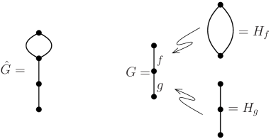
Figure 4.

We have

$$\sum_{s\in\mathcal{S}(G)}a^{k(s)}\left(\prod_{e\in s}\phi_{e}^{(1)}\right)\left(\prod_{e\notin s}\phi_{e}^{(2)}\right)=a\phi_{f}^{(1)}\phi_{g}^{(1)}+a^{2}\phi_{f}^{(1)}\phi_{g}^{(2)}+a^{2}\phi_{f}^{(2)}\phi_{g}^{(1)}+a^{3}\phi_{f}^{(2)}\phi_{g}^{(2)},$$

$$\phi_{f}^{(1)}(a,b)=b^{2}+2b,\quad\phi_{f}^{(2)}(a,b)=1,\quad\phi_{g}^{(1)}(a,b)=b^{2},\quad\phi_{g}^{(2)}(a,b)=2b+a.$$

Therefore

$$\sum_{s\in\mathcal{S}(G)}a^{k(s)}\left(\prod_{e\in s}\phi_{e}^{(1)}\right)\left(\prod_{e\notin s}\phi_{e}^{(2)}\right) = a(b^{2}+2b)b^{2}+a^{2}(b^{2}+2b)(2b+a)+a^{2}(1)b^{2}+a^{3}(1)(2b+a)$$

$$= ab^{4}+2ab^{3}+a^{2}b^{2}+2a^{2}b^{3}+a^{3}b^{2}+4a^{2}b^{2}+2a^{3}b+2a^{3}b+a^{4}$$

$$= \sum_{\hat{s}\in\mathcal{S}(\widehat{G})}a^{k(\hat{s})}b^{e(\hat{s})}$$

as required.

Recalling the definition of the multivariate Tutte polynomial (4), we see that Lemma 2 can be written as

(8) $$Z(\widehat{G};a,b)=\left(\prod_{e\in E}\phi_{e}^{(2)}\right)Z\left(G;a,\left\{\phi_{e}^{(1)}/\phi_{e}^{(2)}\right\}_{e\in E}\right).$$

It remains to express $\phi_{e}^{(1)}$ and $\phi_{e}^{(2)}$ in terms of the Tutte polynomials of certain graphs.

Consider the graph $A_{e}$, defined in Notation 1. The states of $A_{e}$ occur in pairs $s$ and $s\cup e$ where $e\notin s$. Suppose we have a state $s$ that does not contain $e$. Then $s$ contributes a term $a^{k(s)}b^{e(s)}$ to the polynomial $Z(A_{e};a,{\bf b})$, where ${\bf b}$ is as in Notation 1. Now $s\cup e$ has one additional edge with variable $x_{e}$ and it will either have $k$ connected components, if $u_{e}$ and $w_{e}$ are contained in the same connected component of the state $s$, or it will have $k-1$ connected components, if $u_{e}$ and $w_{e}$ lie in different components of $s$. Thus we may write

$$Z(A_{e};a,{\bf b}) =(1+x_{e})\sum_{s\in\mathcal{S}^{1}(H_{e})}a^{k(s)}b^{e(s)}+(1+a^{-1}x_{e})\sum_{s\in\mathcal{S}^{2}(H_{e})}a^{k(s)}b^{e(s)}$$

$$=(1+x_{e})a\phi_{e}^{(1)}+(1+a^{-1}x_{e})a^{2}\phi_{e}^{(2)}.$$

By separating the terms containing $x_{e}$ we can also write

$$Z(A_{e};a,{\bf b})=Z(H_{e};a,b)+x_{e}Z(A_{e}/e;a,b).$$

So we can determine $\phi_{e}^{(1)}$ and $\phi_{e}^{(2)}$ as the unique solution to the equations

$$a\phi_{e}^{(1)}+a^{2}\phi_{e}^{(2)} =Z(H_{e};a,b)$$

$$a\phi_{e}^{(1)}+a\phi_{e}^{(2)} =Z(A_{e}/e;a,b).$$

Collecting this together we have:

Theorem 1.

Let $\widehat{G}$ be a graph which has been obtained from the graph $G=(V,E)$ by taking successive two-sums along each edge $e=(u_{e},w_{e})\in E$ with graphs $A_{e}$. In addition, let $H_{e}$ be the graph $A_{e}$ with the edge $e=(u_{e},w_{e})$ deleted. Then

$$Z(\widehat{G};a,b)=\left(\prod_{e\in E}g_{e}\right)Z\left(G;a,\left\{f_{e}/g_{e}\right\}_{e\in E}\right).$$

where $f_{e}$ and $g_{e}$ are the solutions to

$$a(f_{e}+ag_{e}) =Z(H_{e};a,b)$$

$$a(f_{e}+g_{e}) =Z(A_{e}/e;a,b).$$

$\Box$

Remark 3.

We note that by making a few trivial changes to the argument, the 2-variable polynomial $Z(\widehat{G};a,b)$ can be replaced by the multivariate Tutte polynomial $Z(\widehat{G};a,{\bf x})$ in the theorem.

Since we were considering 2-decompositions of graphs where each $H_{e}$ was allowed to be distinct we were forced into considering the multivariate Tutte polynomial: we needed some way of recording which $H_{e}$ went where. However, if we insist that all of the graphs $H_{e}$ are equal to $H$ say, then we do not need the multivariate Tutte polynomial and we have

Corollary 1.

$$Z(G\otimes A;a,b)=(g)^{e(G)}Z\left(a,f/g\right).$$

where $f$ and $g$ are the solutions to

$$a(f+ag) =Z(H;a,b)$$

$$a(f+g) =Z(A/e;a,b).$$

Example 2.

Let $A=C_{3}$, the 3-cycle. Then $g=a+2b$ and $f=b^{2}$ and we have

$$Z(G\otimes C_{3};a,b)=(a+2b)^{e(G)}Z(G;a,b^{2}/(a+2b)).$$

Since $Z(F)$ is just a rewriting of the Tutte polynomial we can use the above corollary to recover Brylawski’s theorem:

Corollary 2.

$$T(G\otimes A;x,y)=(h)^{n(G)}(h^{\prime})^{r(G)}T\left(G;T(H;x,y)/h^{\prime},T(A/e;x,y)/h\right),$$

where $h$ and $h^{\prime}$ are the unique solutions to

$$(x-1)h+h^{\prime} =T(H;x,y)$$

$$h+(y-1)h^{\prime} =T(A/e;x,y).$$

Proof.

First of all note the identity

(9) $$T(F;x,y)=(x-1)^{-k(F)}(y-1)^{-v(F)}Z(F;(x-1)(y-1),y-1),$$

for any graph $F$. This rewriting allows us to apply Corollary 1 to the Tutte polynomial $T(G\otimes A;x,y)$ as follows.

$$\begin{split}T(G\otimes A;x,y)&=(x-1)^{-k(G\otimes A)}(y-1)^{-v(G\otimes A)}Z(G\otimes A;(x-1)(y-1),y-1)\\ &=(x-1)^{-k(G\otimes A)}(y-1)^{-v(G\otimes A)}g^{e(G)}Z(G;(x-1)(y-1),f/g)\\ &=(x-1)^{-k(G\otimes A)}(y-1)^{-v(G\otimes A)}g^{e(G)}(f/g)^{v(G)}((x-1)(y-1)g/f)^{k(G)}\\ &\hskip 227.62204ptT\left(G;\frac{(x-1)(y-1)g+f}{f},\frac{f+g}{g}\right),\end{split}$$

where $f$ and $g$ are the solutions to the equations of Corollary 1.

Now we set

$$h:=(x-1)^{-k(H)+1}(y-1)^{-v(H)+2}g,\quad h^{\prime}:=(x-1)^{-k(H)+1}(y-1)^{-v(H)+1}f.$$

Our definition of the tensor product has the effect of making $k(H)=k(A/e)$. Also, $v(A/e)=v(H)-1$, and so by (9) the linear equations of Corollary 1 become

$$(x-1)h+h^{\prime} =T(H;x,y)$$

$$h+(y-1)h^{\prime} =T(A/e;x,y)$$

as required. The expression for the Tutte polynomial above becomes

$$T(G\otimes A;x,y)=(x-1)^{-k(G\otimes A)}(y-1)^{-v(G\otimes A)}(x-1)^{(k(H)-1)e(G)}(y-1)^{(v(H)-2)e(G)}\\ h^{e(G)}\left(\frac{(y-1)h^{\prime}}{h}\right)^{v(G)}\left(\frac{(x-1)h}{h^{\prime}}\right)^{k(G)}T\left(G;\frac{(x-1)(y-1)g+f}{f},\frac{f+g}{g}\right).$$

It is easily seen that $v(G\otimes A)=(v(H)-2)e(G)+v(G)$ and $k(G\otimes A)=(k(H)-1)e(G)+k(G)$, and the result follows by cancelling terms. ∎

Remark 4.

In the definition of the tensor product of two graphs we insisted that the vertices $u$ and $w$ of the distinguished edge $e$ of $A$ lay in the same connected component of $H$. This restriction was not used in the proof of Corollary 1, but it was needed in Corollary 2. However if we remove this condition, then we can improve Corollary 1 as follows:

$$T(G\otimes A;x,y)=(h)^{n(G)}(h^{\prime})^{r(G)}T\left(G;T(H;x,y)/h^{\prime},T(A/e;x,y)/((x-1)^{\varepsilon}h)\right),$$

where $h$ and $h^{\prime}$ are the unique solutions to

$$(x-1)h+h^{\prime} =T(H;x,y)$$

$$(x-1)^{\varepsilon}\left(h+(y-1)h^{\prime}\right) =T(A/e;x,y),$$

and $\varepsilon:=k(H)-k(A/e)$. Similar statements will hold for Corollary 3.

4. The Bollobás-Riordan polynomial I: embedding in a neighbourhood

We will begin our study of the Bollobás-Riordan polynomial of 2-decomposable ribbon graphs with a particularly pleasing special case.

Throughout this section $\widehat{G}$ will denote an embedded graph with a 2-decomposition $\left(G,\{H_{e}\}_{e\in E}\right)$, where $G$ is embedded. We will further assume that each graph $H_{e}$ is embedded in a neighbourhood of the edge $e$ of the embedded graph $G$ in the formation of $\widehat{G}$. This restriction on the embedding of $\widehat{G}$ imposes a very strong connection between the topology of $\widehat{G}$ and $G$ which we will use to our advantage.

4.1. Decomposing the states

We proceed as in the case of the Tutte polynomial. A state $\hat{s}\in\mathcal{S}(\widehat{G})$ uniquely determines and is uniquely determined by a set of states $\{s_{e}\in\mathcal{S}(H_{e})\}_{e\in E}$. Again each graph $H_{e}$ has two distinguished vertices $u_{e}$ and $w_{e}$ which are also vertices of $G$. For each $e\in E$ we partition the states of $\mathcal{S}(H_{e})$ into two subsets: $\mathcal{S}^{1}(H_{e})$, which consists of all states in $\mathcal{S}(H_{e})$ in which $u_{e}$ and $w_{e}$ lie in the same connected component; and $\mathcal{S}^{2}(H_{e})$, which consists of all states in $\mathcal{S}(H_{e})$ in which $u_{e}$ and $w_{e}$ lie in different connected components.

Given a state $\hat{s}\in\mathcal{S}(\widehat{G})$, which determines a unique set of states $\{s_{e}\in\mathcal{S}(H_{e})\}_{e\in E}$, construct a state of $G$ by removing an edge $e=(u_{e},w_{e})$ from $G$ if and only if the state $s_{e}$ belongs to the partition $\mathcal{S}^{2}(H_{e})$. This is exactly the construction used in Section 3 to study the Tutte polynomial.

Conversely, given a state $s\in\mathcal{S}(G)$ and a copy of the template $G$, if we replace the edges of $G$ which are also in the state $s$ with elements of $\mathcal{S}^{1}(H_{e})$, and the other edges of $G$ with elements of $\mathcal{S}^{2}(H_{e})$, we obtain a state in $\mathcal{S}(\widehat{G})$. Clearly, each state of $\widehat{G}$ is uniquely obtained in this way.

Lemma 3.

If a state $\hat{s}$ of the embedded graph $\widehat{G}$ is decomposed into states $s\in\mathcal{S}(G)$, $s_{e}\in\mathcal{S}^{1}(H_{e})\cup\mathcal{S}^{2}(H_{e})$, $e\in E$ by the decomposition above, then

$$k(\hat{s})=\sum_{e\in E}k(s_{e})-|\{s_{e}\in\mathcal{S}^{1}(H_{e})\}|-2|\{s_{e}\in\mathcal{S}^{2}(H_{e})\}|+k(s)$$

and

$$\partial(\hat{s})=\sum_{e\in E}\partial(s_{e})-|\{s_{e}\in\mathcal{S}^{1}(H_{e})\}|-2|\{s_{e}\in\mathcal{S}^{2}(H_{e})\}|+\partial(s),$$

where $\partial$ counts the boundary components of the associated ribbon graphs.

To prove this lemma we introduce some notation, which is also useful later. The ribbon graph $\widehat{G}$ is obtained from $G$ by replacing each ribbon $e$ with $H_{e}$. The two ends $\{0,1\}\times I$ of a ribbon $e$ induce two arcs on the incident discs $u_{e}$ and $w_{e}$ ($u_{e}$ and $w_{e}$ may be the same vertex). Denote these two arcs by $m_{e}$ and $n_{e}$. We may then view the replacement of the ribbon $e$ with $H_{e}$ as the operation which identifies an arc on the disc $u_{e}$ of $H_{e}$ with one of the arcs $n_{e}$ or $m_{e}$, and an arc on $w_{e}$ of $H_{e}$ with the other. We also denote these two arcs in $H_{e}$ by $n_{e}$ and $m_{e}$ according to their identification. (Note that by definition the discs $u_{e}$ and $w_{e}$ in $H_{e}$ are distinct.) An example is shown in Figure 5.

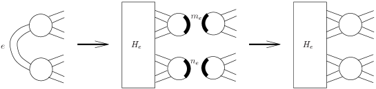
Figure 5.

When the vertices $u_{e}$ and $w_{e}$ of $H_{e}$ and $G$ are identified in the formation of $\widehat{G}$, the boundary components and the connected components containing the marked points $m_{e}$ are merged, and the boundary and connected components containing the marked points $n_{e}$ are merged.

Notice that in the ribbon graph $H_{e}$, either $m_{e}$ and $n_{e}$ belong to the same boundary component, in which case they also belong to the same connected component; or $m_{e}$ and $n_{e}$ belong to distinct boundary components and may or may not belong to the same connected component. For example, in the ribbon graph $T-e$ of Figure 7, $m_{e}$ and $n_{e}$ will belong to different boundary components but the same connected component. In this section we insist that each ribbon graph $H_{e}$ embeds into a neighbourhood of the edge $e$. This means that $H_{e}$ and $A_{e}$ are planar. We then have

$$2k(A_{e})-\partial(A_{e})+e(A_{e})-v(A_{e})=0=2k(H_{e})-\partial(H_{e})+e(H_{e})-v(H_{e}).$$

This gives the relation

$$2k(A_{e})-\partial(A_{e})=2k(H_{e})-\partial(H_{e})-1.$$

Then if $m_{e}$ and $n_{e}$ belong to distinct boundary components in $H_{e}$, we have $\partial(A_{e})=\partial(H_{e})-1$. Therefore $k(A_{e})=k(H_{e})-1$ so $m_{e}$ and $n_{e}$ belong to distinct connected components.

This tells us that (under the embedding condition used in this section) the marked points $m_{e}$ and $n_{e}$ in $H_{e}$ belong to the same boundary component if and only if they belong to the same connected component.

Proof of Lemma 3..

The connectivity relation follows from Lemma 1.

As for the second identity, each boundary component of $s\in\mathcal{S}(G)$ corresponds to a boundary component of $\hat{s}\in\mathcal{S}(\widehat{G})$. To see why this is, with reference to Figure 5, let $a_{e}$ and $a_{e}^{\prime}$ be the two endpoints of the arcs $m_{e}$ and $b_{e}$ and $b_{e}^{\prime}$ be the endpoints of the arcs $n_{e}$. The points $a_{e},a_{e}^{\prime},b_{e},b_{e}^{\prime}$ induce points on the boundary of $G$, $\widehat{G}$, and $H_{e}$, and on the states $\hat{s},s$, and $s_{e}$. Now consider a boundary component of $s$. If this boundary component does not contain any of the points $a_{e},a_{e}^{\prime},b_{e},b_{e}^{\prime}$ then there is a naturally corresponding boundary component in $\hat{s}$. If the boundary cycle contains any of the points $a_{e},a_{e}^{\prime},b_{e},b_{e}^{\prime}$ then there is a corresponding boundary cycle in $\hat{s}$ that contains the same set of points. This sets up a natural correspondence between the boundary components in $s$ and a set of boundary components of $\hat{s}$. However, $\hat{s}$ has extra boundary components arising from the states $s_{e}\in\mathcal{S}^{1}(H_{e})\cup\mathcal{S}^{2}(H_{e})$. These extra boundary components are precisely the unmarked boundary components in the states $s_{e}\in\mathcal{S}^{1}(H_{e})\cup\mathcal{S}^{2}(H_{e})$, $e\in E$. Since the points $a_{e},a_{e}^{\prime},b_{e},b_{e}^{\prime}$ belong to the same boundary component if and only if they belong to the same connected component, we have that for each $e\in E$ for which $s_{e}\in\mathcal{S}^{1}(H_{e})$, there are $\partial(s_{e})-1$ unmarked boundary components; and for each $e\in E$ for which $s_{e}\in\mathcal{S}^{2}(H_{e})$, there are $\partial(s_{e})-2$ unmarked boundary components. Therefore

$$\partial(\hat{s})=\partial(s)+\sum_{\begin{subarray}{c}e\in E\\ s_{e}\in\mathcal{S}^{1}(H_{e})\end{subarray}}(\partial(s_{e})-1)+\sum_{\begin{subarray}{c}e\in E\\ s_{e}\in\mathcal{S}^{2}(H_{e})\end{subarray}}(\partial(s_{e})-2).$$

The lemma then follows. ∎

4.2. An expansion for the Bollobás-Riordan polynomial

We will consider the following state sums:

(10) $$\begin{array}[]{l}\eta_{e}^{(1)}(a,b,c):=\sum_{s\in\mathcal{S}^{1}(H_{e})}a^{k(s)-1}b^{e(s)}c^{\partial(s)-1},\\ \eta_{e}^{(2)}(a,b,c):=\sum_{s\in\mathcal{S}^{2}(H_{e})}a^{k(s)-2}b^{e(s)}c^{\partial(s)-2}.\end{array}$$

The following lemma is analogous to Lemma 2.

Lemma 4.

Let $\left(G,\{H_{e}\}_{e\in E}\right)$ be a 2-decomposition of $\widehat{G}$ then

(11) $$Z(\widehat{G};a,b,c)=\left(\prod_{e\in E}(\eta_{e}^{(2)})\right)Z\left(G;a,\left\{\eta_{e}^{(1)}/\eta_{e}^{(2)}\right\}_{e\in E},c\right).$$

The proof of this lemma is a direct generalization of the proof of Lemma 2 (using the additional relation $\partial(\hat{s})=\partial(s)+\sum(\partial(s_{e})-2)+\sum(\partial(t_{e})-1)$ arising from Lemma 3), and is therefore omitted.

To find a formula for $Z(\widehat{G})$ it remains to determine $\eta_{e}^{(2)}$ and $\eta_{e}^{(1)}$.

Since the edge set of $H_{e}$ is a subset of the edge set of $A_{e}$, we may view states of $H_{e}$ as states of $A_{e}$. The states of $A_{e}$ can then be partitioned into four subsets

(12) $$\begin{array}[]{ll}\mathcal{S}^{1}(H_{e}),&\mathcal{T}^{1}(H_{e}):=\{s\cup e|s\in\mathcal{S}^{1}(H_{e})\}\\ \mathcal{S}^{2}(H_{e}),&\mathcal{T}^{2}(H_{e}):=\{s\cup e|s\in\mathcal{S}^{2}(H_{e})\}.\end{array}$$

Consider the effect of the insertion of the edge $e$ in a state of $H_{e}$ on the numbers of connected components, edges, and boundary cycles. There are two cases. If $s_{e}\in\mathcal{S}^{1}(H_{e})$ then the insertion of $e$ increases the number of boundary cycles by one, so that if $s_{e}$ contributes the term $a^{k}b^{e}c^{\partial}$ to the Bollobás-Riordan polynomial then the state obtained by inserting $e$ contributes $a^{k}(b^{e}x_{e})c^{\partial+1}$. If $s_{e}\in\mathcal{S}^{2}(H_{e})$ then the insertion of $e$ also decreases the number of boundary cycles by one and the number of connected components by one. This means that if $s_{e}$ contributes the term $a^{k}b^{e}c^{\partial}$ to the Bollobás-Riordan polynomial then the state obtained by inserting $e$ contributes $a^{k-1}(b^{e}x_{e})c^{\partial-1}$.

We can now separate the terms in $Z(A_{e};a,{\bf b},c)$ (with ${\bf b}$ as in Notation 1) arising from the four subsets in the partition and write

$$Z(A_{e};a,{\bf b},c)=(x_{e}c+1)\sum_{s\in\mathcal{S}^{1}(H_{e})}a^{k(s)}b^{e(s)}c^{\partial(s)}+(x_{e}a^{-1}c^{-1}+1)\sum_{s\in\mathcal{S}^{2}(H_{e})}a^{k(s)}b^{e(s)}c^{\partial(s)},$$

or

$$Z(A_{e};a,{\bf b},c)=(x_{e}c+1)ac\;\eta_{e}^{(1)}+(x_{e}a^{-1}c^{-1}+1)a^{2}c^{2}\;\eta_{e}^{(2)}.$$

Writing this as a linear equation in $x_{e}$, and using the deletion-contraction relation (6), we have

(13) $$ac\left(\eta_{e}^{(1)}+ac\eta_{e}^{(2)}\right)+ac\left(c\eta_{e}^{(1)}+\eta_{e}^{(2)}\right)x_{e}=Z(H_{e};a,b,c)+x_{e}Z(A_{e}/e;a,b,c).$$

This gives rise to a system of equations

(14) $$\begin{split}ac\left(\eta_{e}^{(1)}+ac\eta_{e}^{(2)}\right)&=Z(H_{e};a,b,c)\\ ac\left(c\eta_{e}^{(1)}+\eta_{e}^{(2)}\right)&=Z(A_{e}/e;a,b,c).\end{split}$$

This pair of linear equations uniquely determines $\eta_{e}^{(1)}$ and $\eta_{e}^{(2)}$. Substitution into equation (11) then gives the following theorem.

Theorem 2.

Let $\widehat{G}$ be an embedded graph with a 2-decomposition $\left(G,\{H_{e}\}_{e\in E}\right)$, such that each graph $H_{e}$ is embedded in a neighbourhood of the edge $e$ of the embedded graph $G$. In addition let $A_{e}$ be the ribbon graph $H_{e}$ with an additional ribbon $e$ joining the vertices $u_{e}$ and $w_{e}$. Then

$$Z(\widehat{G};a,b,c)=(ac)^{-e(G)}\left(\prod_{e\in E}g_{e}\right)Z\left(G;a,\left\{f_{e}/g_{e}\right\}_{e\in E},c\right).$$

where $f_{e}$ and $g_{e}$ are the solutions to

$$acg_{e}+f_{e} =Z(H_{e};a,b,c)$$

$$g_{e}+cf_{e} =Z(A_{e}/e;a,b,c).$$

$\Box$

We may use this to find a result analogous to Corollary 2.

Corollary 3.

Let $G=(V,E)$ be a ribbon graph, $A$ be a planar ribbon graph, and $H=A\backslash e$. Then

$$R(G\otimes A;\alpha,\beta,\gamma)=(h)^{n(G)}(h^{\prime})^{r(G)}R\left(G;\frac{R(H;\alpha,\beta,\gamma)}{h^{\prime}},\frac{\beta h^{\prime}}{h},\gamma\right),$$

where $h$ and $h^{\prime}$ are the unique solutions to

$$h+\beta h^{\prime} =R(A/e;\alpha,\beta,\gamma)$$

$$(\alpha-1)h+h^{\prime} =R(H;\alpha,\beta,\gamma).$$

Proof.

The proof is similar to that of Corollary 2. By (5) we have

$$R(G\otimes A;\alpha,\beta,\gamma)=(\alpha-1)^{-k(G\otimes A)}(\beta\gamma)^{-v(G\otimes A)}Z\left(G\otimes A;(\alpha-1)\beta\gamma^{2},\beta\gamma,\gamma^{-1}\right).$$

An application of the theorem gives

$$R(G\otimes A;\alpha,\beta,\gamma)=(\alpha-1)^{-k(G\otimes A)}(\beta\gamma)^{-v(G\otimes A)}g^{e(G)}Z\left(G;(\alpha-1)\beta\gamma^{2},f/g,\gamma^{-1}\right),$$

where $f$ and $g$ are the solutions to

$$(\alpha-1)\beta\gamma(f+(\alpha-1)\beta\gamma g) =Z\left(H;(\alpha-1)\beta\gamma^{2},\beta\gamma,\gamma^{-1}\right),$$

$$(\alpha-1)\beta\gamma(\gamma^{-1}f+g) =Z\left(A/e;(\alpha-1)\beta\gamma^{2},\beta\gamma,\gamma^{-1}\right).$$

(Note that the $(ac)^{-e(G)}=((\alpha-1)\beta\gamma)^{-e(G)}$ factor has been incorporated into these equations.)

By a second application of (5) we can rewrite the above as

$$R(G\otimes A;\alpha,\beta,\gamma)=(\alpha-1)^{-k(G\otimes A)}(\beta\gamma)^{-v(G\otimes A)}g^{e(G)}\left(\frac{(\alpha-1)\beta\gamma g}{f}\right)^{k(G)}\left(\frac{f}{g}\right)^{v(G)}R\left(G;\frac{(\alpha-1)\beta\gamma g+f}{f},\frac{f}{\gamma g},\gamma\right).$$

Then, just as in the proof of Corollary 2, making the substitution

$$h:=(\alpha-1)^{-k(H)+1}(\beta\gamma)^{-v(H)+2}g,\quad h^{\prime}:=(\alpha-1)^{-k(H)+1}(\beta\gamma)^{-v(H)+1}f,$$

remembering that $v(G\otimes A)=(v(H)-2)e(G)+v(G)$ and $k(G\otimes A)=(k(H)-1)e(G)+k(G)$, and cancelling terms, we have

$$R(G\otimes A;\alpha,\beta,\gamma)=(h)^{n(G)}(h^{\prime})^{r(G)}R\left(G;((\alpha-1)h+h^{\prime})/h^{\prime},\beta h^{\prime}/h,\gamma\right).$$

Now using (5) and noting that $k(H)=k(A/e)$ and $v(A/e)=v(H)-1$, the linear equations can be written as

$$h+\beta h^{\prime}=R(A/e;\alpha,\beta,\gamma),\quad(\alpha-1)h+h^{\prime}=R(H;\alpha,\beta,\gamma).$$

∎

We use this corollary to extend our Example 2.

Example 3.

Let $A=C_{3}$, the 3-cycle. Then $h=\alpha+1$ and $h^{\prime}=1$ and we have $R(G\otimes C_{3};\alpha,\beta,\gamma)=(\alpha+1)^{n(G)}R(G;\alpha^{2},\beta/(\alpha+1),\gamma)$. See also [17] for a proof of this fact using knot theory.

The following is an important application of our results. It provides a method for constructing infinitely many pairs of distinct ribbon graphs with the same Bollobás-Riordan polynomial.

Corollary 4.

Let $G\otimes H$ and $G^{\prime}\otimes H$ be two embedded graphs with the property that each copy of $H$ is embedded in the neighbourhood of an edge. Then if $R(G;a,b,c)=R(G^{\prime};a,b,c)$, $R(G\otimes H;a,b,c)=R(G^{\prime}\otimes H;a,b,c)$.

Proof.

This follows from the previous corollary because if $R(G)=R(G^{\prime})$ then, by setting $c=1$, $T(G)=T(G^{\prime})$, and since the rank and nullity of a graph can be recovered from its Tutte polynomial, we have $r(G)=r(G^{\prime})$ and $n(G)=n(G^{\prime})$. ∎

5. The Bollobás-Riordan polynomial II: the general case

We begin with an informal discussion of the main ideas in this section. Consider the construction of a ribbon graph $\widehat{G}$ from the 2-decomposition $\left(G,\{H_{e}\}_{e\in E}\right)$ locally at an edge $e=(u,w)$ of the template $G$. We will think of the construction of $\widehat{G}$ as the identification of the marked points $m$ and $n$ on the vertices $u$ and $w$ of $H_{e}$ with the corresponding marked points $m$ and $n$ on the vertices $u$ and $w$ of the template $G\backslash e$.

Begin by partitioning $\mathcal{S}(H_{e})$ according to the boundary and connected components containing the marked points $m$ and $n$ on the vertices $u$ and $v$: we let $\ddot{\mathcal{S}}^{2}(H_{e})$ be the set of states of $H_{e}$ in which $m$ and $n$ lie in different connected and different boundary components; $\bar{\mathcal{S}}^{1}(H_{e})$ the states in which $m$ and $n$ lie in the same connected and same boundary components; and $\ddot{\mathcal{S}}^{1}(H_{e})$ the states in which $m$ and $n$ lie in the same connected component but different boundary components.

We would like to define a replacement operation on $\mathcal{S}(G)$ to construct $\mathcal{S}(\widehat{G})$, but we run into a problem. The edge $e$ is either in a state of $G$, in which case we can glue in states from $\bar{\mathcal{S}}^{1}(H_{e})$ (reflecting the fact that $m$ and $n$ lie in the same connected and same boundary components), or $e$ is not in a state of $G$, in which case we can glue in states from $\ddot{\mathcal{S}}^{2}(H_{e})$ (reflecting the fact that $m$ and $n$ lie in different connected and different boundary components). No states of $G$ ever reflect the fact that the markings $m$ and $n$ in $H_{e}$ can lie in different boundary components and the same connected component, so in this construction we never glue in any states from $\ddot{\mathcal{S}}^{1}(H_{e})$.

To get around this problem we replace each edge $e$ in $G$ with an edge $g_{e}$ and a loop $f_{e}$ as in Figure 7, to obtain a graph $\widetilde{G}$. Then there is a subset of the edges $\{f_{e},g_{e}\}$ for each choice of $e\in E$, such that the connectivity and boundary connectivity of the markings $m_{e}$ and $n_{e}$ in $\widetilde{G}$ correspond to the connectivity and boundary connectivity of the markings $m_{e}$ and $n_{e}$ in each of $\ddot{\mathcal{S}}^{2}(H_{e})$, $\ddot{\mathcal{S}}^{1}(H_{e})$ and $\bar{\mathcal{S}}^{1}(H_{e})$. Define a replacement operation as follows: $\{g_{e}\}$ is replaced by states from $\bar{\mathcal{S}}^{1}(H_{e})$; $\{f_{e},g_{e}\}$ by states from $\ddot{\mathcal{S}}^{1}(H_{e})$; and the states $\emptyset$ and $\{f_{e}\}$ are replaced by states from $\ddot{\mathcal{S}}^{2}(H_{e})$. The considerations above show that every element of $\mathcal{S}(\widehat{G})$ is obtained from $\mathcal{S}(\widetilde{G})$ by this operation. However, the states are not obtained uniquely: we have two configurations, $\emptyset$ and $\{f_{e}\}$, for which we substitute states from $\ddot{\mathcal{S}}^{2}(H_{e})$. So rather than dealing with $\mathcal{S}(\widetilde{G})$ we will deal with equivalence classes in this set in which we identify the states containing $f_{e}$ but not $g_{e}$, or neither $f_{e}$ or $g_{e}$. Our replacement operation will then give a construction of $\mathcal{S}(\widehat{G})$ from the sets $\mathcal{S}(\widetilde{G})/\sim$ and $\ddot{\mathcal{S}}^{2}(H_{e})$, $\ddot{\mathcal{S}}^{1}(H_{e})$ and $\bar{\mathcal{S}}^{1}(H_{e})$, $e\in E$. We will now do this formally.

5.1. Decomposing the ribbon graph

We view the construction of $\widehat{G}$ in terms of the identification of arcs $n_{e}$ and $m_{e}$ as described in Subsection 4.1 and by Figure 5.

Given a state $\hat{s}\in\mathcal{S}(\widehat{G})$ and a 2-decomposition $\left(G,\{H_{e}\}_{e\in E}\right)$ for the ribbon graph $\widehat{G}$, the state $\hat{s}$ uniquely determines a set of states $\{s_{e}\in\mathcal{S}(H_{e})\}_{e\in E}$. Partition each $\mathcal{S}(H_{e})$ as follows. Let $s_{e}\in\mathcal{S}(H_{e})$, then $s_{e}\in\bar{\mathcal{S}}(H_{e})$ if and only if $m_{e}$ and $n_{e}$ belong to the same boundary component. Otherwise $s_{e}\in\ddot{\mathcal{S}}(H_{e})$. (So the accent on $\mathcal{S}$ has one component if and only if $m_{e}$ and $n_{e}$ belong to one boundary component.) These two situations are indicated in Figure 6.

$$\psfig{width=113.81102pt}\;\;,\hskip 56.9055pt\psfig{width=113.81102pt}$$

Figure 6.

We want to include connectivity information in the above partition. We do this by taking its intersection with the partition of Subsection 3.1. Let $\left(G,\{H_{e}\}_{e\in E}\right)$ be a 2-decomposition for the ribbon graph $\widehat{G}$ and $\mathcal{S}^{1}(H_{e})$, $\mathcal{S}^{2}(H_{e})$, $\ddot{\mathcal{S}}(H_{e})$ and $\bar{\mathcal{S}}(H_{e})$ be the sets described in Subsections 3.1 and above. Define

$$\begin{array}[]{ll}\bar{\mathcal{S}}^{1}(H_{e}):=\mathcal{S}^{1}(H_{e})\cap\bar{\mathcal{S}}(H_{e}),&\ddot{\mathcal{S}}^{1}(H_{e}):=\mathcal{S}^{1}(H_{e})\cap\ddot{\mathcal{S}}(H_{e}),\\ \bar{\mathcal{S}}^{2}(H_{e}):=\mathcal{S}^{2}(H_{e})\cap\bar{\mathcal{S}}(H_{e}),&\ddot{\mathcal{S}}^{2}(H_{e}):=\mathcal{S}^{2}(H_{e})\cap\ddot{\mathcal{S}}(H_{e}).\end{array}$$

Notice that $\bar{\mathcal{S}}^{2}(H_{e})=\emptyset$ and $\ddot{\mathcal{S}}^{1}(H_{e})\cup\ddot{\mathcal{S}}^{2}(H_{e})=\ddot{\mathcal{S}}(H_{e})$. We have

Lemma 5.

$\bar{\mathcal{S}}^{1}(H_{e})$, $\ddot{\mathcal{S}}^{1}(H_{e})$ and $\ddot{\mathcal{S}}^{2}(H_{e})$ partition the sets $\mathcal{S}(H_{e})$, $e\in E$. Moreover every state of $\widehat{G}$ can be uniquely obtained by the replacement of an edge in a state of $G$ by an element of $\bar{\mathcal{S}}^{1}(H_{e})$ and the replacement of a non-edge in that state of $G$ with an element of $\ddot{\mathcal{S}}^{1}(H_{e})\cup\ddot{\mathcal{S}}^{2}(H_{e})$. $\Box$

Rather than considering states of the template $G$, we need to consider states of a slightly more complex ribbon graph. We define the ribbon graph $\widetilde{G}$ to be the tensor product (along $e$) of the template $G$ with the ribbon graph $T$ defined by Figure 7(a), having the specified edge-labels. We will see that it does not matter if the loop is at the vertex labelled $u_{e}$ or $w_{e}$. An example of $\widetilde{G}$ is shown in Figure 7(b).

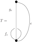
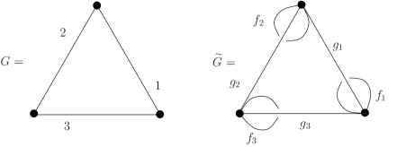
Figure 7.

We want to construct the set of states $\mathcal{S}(\widehat{G})$ by replacing states in $\mathcal{S}(\widetilde{G})$ by states from $\mathcal{S}(H_{e})=\bar{\mathcal{S}}^{1}(H_{e})\cup\ddot{\mathcal{S}}^{1}(H_{e})\cup\ddot{\mathcal{S}}^{2}(H_{e})$.

We will say that two states of $\widetilde{G}=G\otimes T$ are equivalent if for some choice of $e$, one state contains neither of the edges $f_{e}$ or $g_{e}$, the other state contains the edge $f_{e}$ but not $g_{e}$, and all of the other edges contained in the two states are the same. This defines an equivalence relation $\sim$ on $\mathcal{S}(\widetilde{G})$. We are interested in the set $\mathcal{S}(\widetilde{G})/\sim$.

We can construct the set of states $\mathcal{S}(\widehat{G})$ by replacing equivalence classes of $\mathcal{S}(\widetilde{G})/\sim$ with $\{\mathcal{S}(H_{e})\}_{e\in E(G)}$ as follows. Given an equivalence class $[s]\in\mathcal{S}(\widetilde{G})/\sim$ choose a representative $s\in[s]$. Then for each choice of $e$, we have the following possibilities in the equivalence class: $s$ contains both $f_{e}$ and $g_{e}$; or $g_{e}$ but not $f_{e}$; or it does not contain $g_{e}$ and may or may not contain $f_{e}$ (these two situations being equivalent).

Construct a state of $\widehat{G}$ using the replacement operation:

• if $s$ contains both of $f_{e}$ and $g_{e}$, remove both of these two edges and glue in a state from $\ddot{\mathcal{S}}^{1}(H_{e})$;

• if a state contains the edge $g_{e}$ but not $f_{e}$, remove the edge $g_{e}$ and glue in a state from $\bar{\mathcal{S}}^{1}(H_{e})$;

• if a state contains the edge $f_{e}$ but not $g_{e}$, remove the edge $f_{e}$ and glue in a state from $\ddot{\mathcal{S}}^{2}(H_{e})$, or if the original state contains neither of the edges $f_{e}$ or $g_{e}$ then glue in a state from $\ddot{\mathcal{S}}^{2}(H_{e})$.

An example of the decomposition of a state of $\widehat{G}$ is shown in Figure 8 where $G=C_{4}$.

The following lemma is clear.

Lemma 6.

$\bar{\mathcal{S}}^{1}(H_{e})$, $\ddot{\mathcal{S}}^{1}(H_{e})$ and $\ddot{\mathcal{S}}^{2}(H_{e})$ partition the sets $\mathcal{S}(H_{e})$, $e\in E$. Moreover every state of $\widehat{G}$ can be uniquely obtained by replacing classes in $\mathcal{S}(\widetilde{G})/\sim$ with elements of $\bar{\mathcal{S}}^{1}(H_{e})$, $\ddot{\mathcal{S}}^{1}(H_{e})$ and $\ddot{\mathcal{S}}^{2}(H_{e})$ in the manner described above. $\Box$

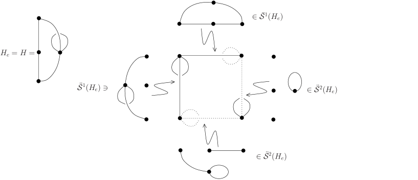
Figure 8.

5.2. An expansion for the Bollobás-Riordan polynomial

We consider the following state sums:

(15) $$\begin{array}[]{l}\Phi_{\widetilde{G}}(a,\{f_{e},g_{e}\}_{e\in E},c):=\sum_{[s]\in\mathcal{S}(\widetilde{G})/\sim}a^{k(s)}\left(\prod_{e\in s}x_{e}\right)c^{\partial(s)},\\ \ddot{\eta}_{e}^{(1)}(a,b,c):=\sum_{s\in\ddot{\mathcal{S}}^{1}(H_{e})}a^{k(s)-1}b^{e(s)}c^{\partial(s)-2},\\ \ddot{\eta}_{e}^{(2)}(a,b,c):=\sum_{s\in\ddot{\mathcal{S}}^{2}(H_{e})}a^{k(s)-2}b^{e(s)}c^{\partial(s)-2},\\ \bar{\eta}_{e}^{(1)}(a,b,c):=\sum_{s\in\bar{\mathcal{S}}^{1}(H_{e})}a^{k(s)-1}b^{e(s)}c^{\partial(s)-1},\end{array}$$

where in the expression for $\Phi_{\widetilde{G}}$ the product is taken over the edges of a representative $s\in[s]$ such that $s$ has the fewest edges in its equivalence class, and $\{x_{e}\}$ denotes the set of labels $\{f_{e},g_{e}\}$ of the edges in $\widetilde{G}$.

We emphasize that we are abusing notation by using $\{f_{e},g_{e}\}$ to denote both the set of edge labels and the set of edge weights. This abuse of notation should cause no confusion.

Lemma 7.

Suppose that a state $\hat{s}$ of $\widehat{G}$ is obtained by replacement from the states $[s]\in\mathcal{S}(\widetilde{G})$, $s_{e}\in\ddot{\mathcal{S}}^{1}(H_{e})$, $t_{e}\in\ddot{\mathcal{S}}^{2}(H_{e})$, and $u_{e}\in\bar{\mathcal{S}}^{1}(H_{e})$ using the decomposition. Then

$$\begin{array}[]{ll}\partial(\hat{s})=&\partial(s)+\sum(\partial(s_{e})-2)+\sum(\partial(t_{e})-2)+\sum(\partial(u_{e})-1),\\ k(\hat{s})=&k(s)+\sum(k(s_{e})-1)+\sum(k(t_{e})-2)+\sum(k(u_{e})-1),\\ e(\hat{s})=&\sum e(s_{e})+\sum e(t_{e})+\sum e(u_{e}),\end{array}$$

where the representative $s\in[s]$ is chosen so that it has the fewest edges in its class.

Proof.

For the first identity, since our representative $s\in[s]\in\mathcal{S}(\widetilde{G})/\sim$ was chosen so that it has the fewest edges in its class, the state $s$ contains an edge $f_{e}$ if and only if it contains the edge $g_{e}$. The argument now follows the proof of Lemma 3: each boundary component of $s\in\mathcal{S}(\widetilde{G})$ corresponds to a boundary component of $\hat{s}\in\mathcal{S}(\widehat{G})$. These are easily seen to be the boundary components of $\hat{s}$ which contain a point $a_{e},a_{e}^{\prime},b_{e},b_{e}^{\prime}$ (with these points defined as in Lemma 3). However $\hat{s}$ has additional boundary components arising from the states $s_{e}$. These extra boundary components of $\hat{s}$ are precisely the boundary components of the $s_{e}$ which do not contain a point $a_{e},a_{e}^{\prime},b_{e},b_{e}^{\prime}$. For each $e$ there are $(\partial(s_{e})-2)$ of these if $s_{e}\in\ddot{\mathcal{S}}^{1}(H_{e})$, $(\partial(t_{e})-2))$ of these if $t_{e}\in\ddot{\mathcal{S}}^{2}(H_{e})$, and $(\partial(u_{e})-1))$ of these if $u_{e}\in\bar{\mathcal{S}}^{1}(H_{e})$. The result follows.

The remaining identities follow similarly (see also the proofs of Lemmas 1 and 3). ∎

We define the linear map $\mathcal{F}:\mathbb{Z}[\{f_{e},g_{e}\}_{e\in E}]\rightarrow\mathbb{Z}[\{\ddot{\eta}_{e}^{(1)},\ddot{\eta}_{e}^{(2)},\bar{\eta}_{e}^{(1)}\}_{e\in E}]$ to be the linear extension of the map

$$\mathcal{F}:\prod_{e\in E}f_{e}^{\alpha_{e}}g_{e}^{\beta_{e}}\mapsto\prod_{e\in E}\left(\ddot{\eta}_{e}^{(1)}\right)^{\alpha_{e}\beta_{e}}\left(\ddot{\eta}_{e}^{(2)}\right)^{(1-\beta_{e})}\left(\bar{\eta}_{e}^{(1)}\right)^{(\beta_{e}-\alpha_{e}\beta_{e})}.$$

For example, $\mathcal{F}$ sends the monomial $f_{1}g_{1}g_{2}\in\mathbb{Z}[f_{1},f_{2},f_{3},g_{1},g_{2},g_{3}]$ to $\ddot{\eta}_{1}^{(1)}\bar{\eta}_{2}^{(1)}\ddot{\eta}_{3}^{(2)}$.

Lemma 8.

$$Z(\widehat{G};a,b,c)=\mathcal{F}\left(\Phi_{\widetilde{G}}\right).$$

Proof.

Let $[s]\in\mathcal{S}(\widetilde{G})/\sim$ and $s\in[s]$ be the representative with the fewest edges in its class. We then know that for each index $e\in E$, $s$ contains both $f_{e}$ and $g_{e}$; or $g_{e}$ but not $f_{e}$; or neither $f_{e}$ nor $g_{e}$. We construct a state of $\widehat{G}$ by replacing the three edge configurations $\{f_{e},g_{e}\}$, $\{g_{e}\}$, and $\emptyset$ of the pair of edges $\{f_{e},g_{e}\}$, with states $s_{e}$ of $\ddot{\mathcal{S}}^{1}(H_{e})$, $\bar{\mathcal{S}}^{1}(H_{e})$, and $\ddot{\mathcal{S}}^{2}(H_{e})$ respectively. Each state of $\widehat{G}$ is uniquely obtained in this way, and the corresponding contribution to $Z(\widehat{G})$ will be

(16) $$a^{k(s)}c^{\partial(s)}\prod_{e\in E}\left(a^{k(s_{e})-1}b^{e(s_{e})}c^{\partial(s_{e})-2}\right)^{\alpha_{e}\beta_{e}}\left(a^{k(s_{e})-2}b^{e(s_{e})}c^{\partial(s_{e})-2}\right)^{1-\beta_{e}}\left(a^{k(s_{e})-1}b^{e(s_{e})}c^{\partial(s_{e})-1}\right)^{\beta_{e}-\alpha_{e}\beta_{e}},$$

where $\alpha_{e}=\left\{\begin{array}[]{ll}1&\text{ if }f_{e}\in s\\ 0&\text{ otherwise}\end{array}\right.$ and $\beta_{e}=\left\{\begin{array}[]{ll}1&\text{ if }g_{e}\in s\\ 0&\text{ otherwise}\end{array}\right.$.

Clearly expression (16) is equal to $\mathcal{F}\left(a^{k(s)}(\prod_{e\in s}x_{e})c^{\partial(s)})\right)$, the contribution of the state $s$ to $\Phi_{\widetilde{G}}$. But it is also equal to

$$a^{k(s)+\sum_{s_{e}\in\ddot{\mathcal{S}}^{1}(H_{e})}(k(s_{e})-1)+\sum_{s_{e}\in\ddot{\mathcal{S}}^{2}(H_{e})}(k(s_{e})-2)+\sum_{s_{e}\in\bar{\mathcal{S}}^{1}(H_{e})}(k(s_{e})-1)}\\ b^{\sum_{s_{e}\in\ddot{\mathcal{S}}^{1}(H_{e})}e(s_{e})+\sum_{s_{e}\in\ddot{\mathcal{S}}^{2}(H_{e})}e(s_{e})+\sum_{s_{e}\in\bar{\mathcal{S}}^{1}(H_{e})}e(s_{e})}\\ c^{\partial(s)+\sum_{s_{e}\in\ddot{\mathcal{S}}^{1}(H_{e})}(\partial(s_{e})-2)+\sum_{s_{e}\in\ddot{\mathcal{S}}^{2}(H_{e})}(\partial(s_{e})-2)+\sum_{s_{e}\in\bar{\mathcal{S}}^{1}(H_{e})}(\partial(s_{e})-1)}.$$

From Lemma 7, this sum is equal to $a^{k(\hat{s})}b^{e(\hat{s})}c^{\partial(\hat{s})}$. By the uniqueness of the decomposition of the states $\hat{s}\in\mathcal{S}(\widehat{G})$ into states of $\mathcal{S}(\widetilde{G})/\sim$ and $\mathcal{S}(H_{e})$, $e\in E$, the result follows on summing over the states. ∎

Notice that the polynomial $Z(\widetilde{G};a,{\bf x},c)$ enumerates all of the states of $\widetilde{G}$. Our next result uses this observation to replace $\Phi_{\widetilde{G}}$ in the above lemma with $Z(\widetilde{G})$.

Lemma 9.

Let $\left(G,\{H_{e}\}_{e\in E}\right)$ be a 2-decomposition of $\widehat{G}$, and $\mathcal{G}:\mathbb{Z}[\{f_{e},g_{e}\}_{e\in E}]\rightarrow\mathbb{Z}[\{\ddot{\eta}_{e}^{(1)},\ddot{\eta}_{e}^{(2)},\bar{\eta}_{e}^{(1)}\}_{e\in E}]$ be the linear extension of the map

$$\mathcal{G}:\prod_{e\in E}f_{e}^{\alpha_{e}}g_{e}^{\beta_{e}}\mapsto\prod_{e\in E}\left(\ddot{\eta}_{e}^{(1)}\right)^{\alpha_{e}\beta_{e}}\left(\frac{1}{2}\ddot{\eta}_{e}^{(2)}\right)^{(1-\beta_{e})}c^{(\alpha_{e}\beta_{e}-\alpha_{e})}\left(\bar{\eta}_{e}^{(1)}\right)^{(\beta_{e}-\alpha_{e}\beta_{e})}.$$

Then

$$Z(\widehat{G};a,b,c)=\mathcal{G}\left(Z(\widetilde{G};a,{\bf x},c)\right).$$

Proof.

We can write the polynomial

$$Z(\widetilde{G};a,{\bf x},c)=\sum_{\tilde{s}\in\widetilde{G}}a^{k(\tilde{s})}c^{\partial(\tilde{s})}\left(\prod_{e\in\tilde{s}}x_{e}\right)$$

as

$$\sum_{\tilde{s}\in\widetilde{G}}a^{k(\tilde{s})}c^{\partial(\tilde{s})}\prod_{e\in\tilde{s}}\left((f_{e}g_{e})^{\alpha_{e}}(f_{e})^{\beta_{e}}(g_{e})^{\gamma_{e}}(1)^{\delta_{e}}\right),$$

where exactly one of $\alpha_{e}$, $\beta_{e}$, $\gamma_{e}$, $\delta_{e}$ is one and all of the others are zero for each $e\in E$.

Now suppose that a state $\tilde{s}$ decomposes into states $s_{e}\in\mathcal{S}(H_{e})$, $e\in E$. Then for any $e$, if $\beta_{e}=1$ or $\delta_{e}=1$ we know that $s_{e}\in\ddot{\mathcal{S}}^{2}(H_{e})$ and since a state containing only $f_{e}$ will have exactly one more boundary component than a state containing neither $f_{e}$ or $g_{e}$, for some $e$, we may write the above formula as

(17) $$\sum_{[\tilde{s}]\in\widetilde{G}/\sim}a^{k(\tilde{s})}c^{\partial(\tilde{s})}\prod_{e\in\tilde{s}}\left((f_{e}g_{e})^{\alpha_{e}}(1+cf_{e})^{\beta_{e}}(g_{e})^{\gamma_{e}}\right),$$

where the representative $\tilde{s}$ is chosen so that it has the fewest edges in its class.

We need to show that the map $\mathcal{G}$ applied to (17) is equal to $\mathcal{F}(\Phi_{\widetilde{G}})$. The state sum $\Phi_{\widetilde{G}}$ can be expressed as

(18) $$\Phi_{\widetilde{G}}=\sum_{[\tilde{s}]\in\widetilde{G}/\sim}a^{k(\tilde{s})}c^{\partial(\tilde{s})}\prod_{e\in\tilde{s}}\left((f_{e}g_{e})^{\alpha_{e}}(1)^{\beta_{e}}(g_{e})^{\gamma_{e}}\right),$$

where the representative $\tilde{s}$ is chosen so that it has the fewest edges in its class, and exactly one of $\alpha_{e}$, $\beta_{e}$, $\gamma_{e}$, $\delta_{e}$ is one and all of the others are zero for each $e\in E$.

There is a clear correspondence between the summands of (17) and (18). In particular, if for some $e$, a summand of (17) contains the expression $(f_{e}g_{e})^{1}(1+cf_{e})^{0}(g_{e})^{0}$ then the corresponding summand of (18) contains a term $(f_{e}g_{e})^{1}(1)^{0}(g_{e})^{0}$ and these terms are mapped by $\mathcal{G}$ and $\mathcal{F}$ respectively to $\ddot{\eta}_{e}^{(1)}$. Also if for some $e$, a summand of (17) contains the expression $(f_{e}g_{e})^{0}(1+cf_{e})^{0}(g_{e})^{1}$ then the corresponding summand of (18) contains a term $(f_{e}g_{e})^{0}(1)^{0}(g_{e})^{1}$ and these terms are mapped by $\mathcal{G}$ and $\mathcal{F}$ respectively to $\bar{\eta}_{e}^{(1)}$. Finally, if for some $e$, a summand of (17) contains the expression $(f_{e}g_{e})^{0}(1+cf_{e})^{1}(g_{e})^{0}$ then the corresponding summand of (18) contains a term $(f_{e}g_{e})^{0}(1)^{1}(g_{e})^{0}$. In this case

$$\mathcal{G}((f_{e}g_{e})^{0}(1+cf_{e})^{1}(g_{e})^{0})=\frac{1}{2}\ddot{\eta}_{e}^{(2)}+c(c^{-1}\frac{1}{2}\ddot{\eta}_{e}^{(2)})=\ddot{\eta}_{e}^{(2)}=\mathcal{F}((f_{e}g_{e})^{0}(1)^{1}(g_{e})^{0}).$$

Hence we see that applying the map $\mathcal{G}$ to (17) will give $\mathcal{F}(\Phi_{\widetilde{G}})$, and then an application of Lemma 8 will give the required identity

$$\mathcal{G}\left(Z(\widetilde{G};a,{\bf x},c)\right)=Z(\widehat{G};a,b,c).$$

∎

It remains to determine $\bar{\eta}_{e}^{(1)}$ , $\ddot{\eta}_{e}^{(1)}$ and $\ddot{\eta}_{e}^{(2)}$.

5.3. Using ribbon graphs

We may view states of $H_{e}$ as states of $A_{e}$. The states of $A_{e}$ can be partitioned into six subsets

(19) $$\begin{array}[]{ll}\ddot{\mathcal{S}}^{1}(H_{e}),&\ddot{\mathcal{T}}^{1}(H_{e}):=\{s\cup e|s\in\ddot{\mathcal{S}}^{1}(H_{e})\}\\ \ddot{\mathcal{S}}^{2}(H_{e}),&\ddot{\mathcal{T}}^{2}(H_{e}):=\{s\cup e|s\in\ddot{\mathcal{S}}^{2}(H_{e})\}\\ \bar{\mathcal{S}}^{1}(H_{e}),&\bar{\mathcal{T}}^{1}(H_{e}):=\{s\cup e|s\in\bar{\mathcal{S}}^{1}(H_{e})\}.\end{array}$$

Consider the effect of the insertion of the edge $e$ into a state of $H_{e}$ on the number of connected components, edges, and boundary components, and the corresponding terms in $Z(H_{e};a,{\bf b},c)$. There are three cases. If $s_{e}\in\ddot{\mathcal{S}}^{1}(H_{e})$ then the insertion of $e$ decreases the number of boundary cycles by one. This means that if $s_{e}$ contributes the term $a^{k}b^{e}c^{\partial}$ to the Bollobás-Riordan polynomial then the state obtained by inserting $e$ contributes $a^{k}(b^{e}x_{e})c^{\partial-1}$. If $s_{e}\in\ddot{\mathcal{S}}^{2}(H_{e})$ then the insertion of $e$ decreases the number of boundary cycles by one and the number of connected components by one. This means that if $s_{e}$ contributes the term $a^{k}b^{e}c^{\partial}$ to the Bollobás-Riordan polynomial then the state obtained by inserting $e$ contributes $a^{k-1}(b^{e}x_{e})c^{\partial-1}$. Finally, if $s_{e}\in\bar{\mathcal{S}}^{1}(H_{e})$ then the insertion of $e$ also increases the number of boundary cycles by one. This means that if $s_{e}$ contributes the term $a^{k}b^{e}c^{\partial}$ to the Bollobás-Riordan polynomial then the state obtained by inserting $e$ contributes $a^{k}(b^{e}x_{e})c^{\partial+1}$.

We can then separate the terms in $Z(A_{e};a,{\bf b},c)$, ${\bf b}$ as in Notation 1, arising from the six subsets in the partition and write:

$$Z(A_{e};a,{\bf b},c)=(x_{e}c^{-1}+1)\sum_{s\in\ddot{\mathcal{S}}^{1}(H_{e})}a^{k(s)}b^{e(s)}c^{\partial(s)}+(x_{e}a^{-1}c^{-1}+1)\sum_{s\in\ddot{\mathcal{S}}^{2}(H_{e})}a^{k(s)}b^{e(s)}c^{\partial(s)}\\ +(x_{e}c+1)\sum_{s\in\bar{\mathcal{S}}^{1}(H_{e})}a^{k(s)}b^{e(s)}c^{\partial(s)}.$$

Rewriting in terms of $\ddot{\eta}_{e}^{(1)},\ddot{\eta}_{e}^{(2)}$, and $\bar{\eta}_{e}^{(1)}$ gives

$$Z(A_{e};a,{\bf b},c)=(x_{e}c^{-1}+1)ac^{2}\;\ddot{\eta}_{e}^{(1)}+(x_{e}a^{-1}c^{-1}+1)a^{2}c^{2}\;\ddot{\eta}_{e}^{(2)}+(x_{e}c+1)ac\;\bar{\eta}_{e}^{(1)}.$$

Writing this as a linear equation in $x_{e}$, and using the deletion-contraction relation (6), we have

(20) $$ac\left(c\ddot{\eta}_{e}^{(1)}+ac\ddot{\eta}_{e}^{(2)}+\bar{\eta}_{e}^{(1)}\right)+ac\left(\ddot{\eta}_{e}^{(1)}+\ddot{\eta}_{e}^{(2)}+c\bar{\eta}_{e}^{(1)}\right)x_{e}=Z(H_{e};a,b,c)+x_{e}Z(A_{e}/e;a,b,c).$$

giving rise to a system of equations

(21) $$\begin{split}ac\left(c\ddot{\eta}_{e}^{(1)}+ac\ddot{\eta}_{e}^{(2)}+\bar{\eta}_{e}^{(1)}\right)&=Z(H_{e};a,b,c)\\ ac\left(\ddot{\eta}_{e}^{(1)}+\ddot{\eta}_{e}^{(2)}+c\bar{\eta}_{e}^{(1)}\right)&=Z(A_{e}/e;a,b,c).\end{split}$$

We need to be able to determine the polynomials $\bar{\eta}_{e}^{(1)}$ , $\ddot{\eta}_{e}^{(1)}$ and $\ddot{\eta}_{e}^{(2)}$ uniquely. When $a=1$ we can solve (21) for $c$ and obtain a formula for $Z(\widehat{G};1,b,c)$, and when $c=1$, we can solve for $a$ to obtain a formula for the Tutte polynomial $Z(\widehat{G};a,b)$. However, in general the system (21) does not have a unique solution. In Section 4 we got around this difficulty by restricting the topology of the ribbon graphs $H_{e}$. In Section 5.4 we will determine the polynomials $\bar{\eta}_{e}^{(1)}$ , $\ddot{\eta}_{e}^{(1)}$ and $\ddot{\eta}_{e}^{(2)}$ by considering geometric ribbon graphs. But before we do this we observe that we could determine these polynomials uniquely if we used multivariate polynomials $Z(H_{e};a,{\bf x},c)$.

Label all of the edges of $A_{e}$ with elements of a set ${\bf x}$ and consider the multivariate Bollobás-Riordan polynomial $Z(A_{e};a,{\bf x},c)$. Each state $s$ of $H_{e}$ is uniquely determined by the set of edges it contains and therefore gives rise to a unique monomial $\prod_{e\in E(s)}x_{e}$ in ${\bf x}$. This in turn determines a unique term of $Z(A_{e};a,{\bf x},c)$. This means that each monomial term in $Z(A_{e};a,{\bf x},c)$ appears exactly once on each side of equation (20) and we can therefore solve (21) by comparing terms. Lemma 9 then gives:

Theorem 3.

Let $\widehat{G}$ be a ribbon graph with the 2-decomposition $\left(G,\{H_{e}\}_{e\in E}\right)$, and let $A_{e}$ be the ribbon graph $H_{e}$ with an additional ribbon $e$ joining the vertices $u_{e}$ and $w_{e}$. Then

$$Z(\widehat{G};a,{\bf x},c)=\mathcal{G}\left(Z\left(\widetilde{G};a,{\bf x},c\right)\right),$$

where $p_{e}$, $q_{e}$ and $r_{e}$ are uniquely determined by the pair of equations

$$cp_{e}+q_{e}+r_{e} =Z(A_{e}/e;a,{\bf x},c)$$

$$p_{e}+acq_{e}+cr_{e} =Z(H_{e};a,{\bf x},c),$$

and $\mathcal{G}$ is induced by

$$\mathcal{G}:\prod_{e\in E}f_{e}^{\alpha_{e}}g_{e}^{\beta_{e}}\mapsto\prod_{e\in E}\left(\frac{r_{e}}{ac}\right)^{\alpha_{e}\beta_{e}}\left(\frac{q_{e}}{2ac}\right)^{(1-\beta_{e})}c^{(\alpha_{e}\beta_{e}-\alpha_{e})}\left(\frac{p_{e}}{ac}\right)^{(\beta_{e}-\alpha_{e}\beta_{e})}.$$

$\Box$

5.4. Geometric ribbon graphs

Let $H_{e}$ be a ribbon graph (so that $t(H_{e})=0$). Previously we considered the ribbon graph $A_{e}$, which consisted of $H_{e}$ with an additional untwisted ribbon $e=(u_{e},w_{e})$. Here we consider the geometric ribbon graph $A_{\tilde{e}}$, which is obtained from $H_{e}$ by inserting a half-twisted ribbon $\tilde{e}$ between the vertices $u_{e}$ and $w_{e}$. This ribbon is inserted into the ribbon graph $H_{e}$ according to the conventions of Notation 1. $A_{\tilde{e}}$ will always denote a geometric ribbon graph constructed from $H_{e}$ in this way. We will only need to distinguish the edge $\tilde{e}$ in $Z(a,{\bf x},c,d)$ so as before, we will denote by ${\bf b}$ the specialization of ${\bf x}$ which sets $x_{e}=b$ for $e\neq q$.

The insertion of the ribbon $\tilde{e}$ into a state $s\in\mathcal{S}(H_{e})$ determines a unique state $\tilde{s}\in\mathcal{S}(A_{\tilde{e}})$. Notice that since $s$ is orientable, $\tilde{s}$ is non-orientable (and $t(\tilde{s})=1$) if and only if the vertices $u_{e}$ and $w_{e}$ lie in the same connected component in $s$. We will use this observation in the proof of the following theorem.

Theorem 4.

Let $\widehat{G}$ be a ribbon graph with the 2-decomposition $\left(G,\{H_{e}\}_{e\in E}\right)$, and let $A_{\tilde{e}}$ be the ribbon graph $H_{e}$ with a half-twisted edge $\tilde{e}=(u_{e},w_{e})$ inserted. Then

$$Z(\widehat{G};a,b,c)=\mathcal{G}\left(Z\left(\widetilde{G};a,{\bf x},c\right)\right)$$

where

$$q_{e}=Z\left(A_{\tilde{e}}/\tilde{e};a,b,c,0\right);$$

$p_{e}$ and $r_{e}$ are uniquely determined by the pair of equations

$$cp_{e}+r_{e} =Z(A_{\tilde{e}}/\tilde{e};a,b,c,1)-Z(A_{\tilde{e}}/\tilde{e};a,b,c,0)$$

$$p_{e}+cr_{e} =Z(H_{e};a,b,c)-acZ(A_{\tilde{e}}/\tilde{e};a,b,c,0);$$

and $\mathcal{G}$ is induced by

$$\mathcal{G}:\prod_{e\in E}f_{e}^{\alpha_{e}}g_{e}^{\beta_{e}}\mapsto\prod_{e\in E}\left(\frac{r_{e}}{ac}\right)^{\alpha_{e}\beta_{e}}\left(\frac{q_{e}}{2ac}\right)^{(1-\beta_{e})}c^{(\alpha_{e}\beta_{e}-\alpha_{e})}\left(\frac{p_{e}}{ac}\right)^{(\beta_{e}-\alpha_{e}\beta_{e})}.$$

Proof.

Just as in the derivation of (21), we consider the effect of the insertion of the edge $\tilde{e}$ into a state of $H_{e}$ on the number of connected components, edges, boundary cycles, and the orientability of the surface. Let $\ddot{\mathcal{S}}^{1}(H_{e})$, $\ddot{\mathcal{S}}^{2}(H_{e})$ and $\bar{\mathcal{S}}^{1}(H_{e})$ be the partition of $\mathcal{S}(H_{e})$ described in Subsection 5.1. Suppose that $s\in\mathcal{S}(H_{e})$. Then if $s\in\ddot{\mathcal{S}}^{1}(H_{e})$ the insertion of $\tilde{e}$ reduces the number of boundary cycles by one and makes the surface non-orientable; if $s\in\ddot{\mathcal{S}}^{2}(H_{e})$ the insertion of $\tilde{e}$ reduces the number of boundary cycles by one and decreases the number of connected components by one; if $s\in\bar{\mathcal{S}}^{1}(H_{e})$ the insertion of $\tilde{e}$ makes the surface non-orientable but the number of boundary cycles and connected components is unchanged.

Now since every state in $\mathcal{S}(A_{\tilde{e}})$ is either a state in $\mathcal{S}(H_{e})$ or a state determined by the insertion of the ribbon $\tilde{e}$ into a state in $\mathcal{S}(H_{e})$, we have

$$Z(A_{\tilde{e}};a,{\bf b},c,t)=(x_{\tilde{e}}c^{-1}t+1)\sum_{s\in\ddot{\mathcal{S}}^{1}(H_{e})}a^{k(s)}b^{e(s)}c^{\partial(s)}+(x_{\tilde{e}}a^{-1}c^{-1}+1)\sum_{s\in\ddot{\mathcal{S}}^{2}(H_{e})}a^{k(s)}b^{e(s)}c^{\partial(s)}\\ +(x_{\tilde{e}}t+1)\sum_{s\in\ddot{\mathcal{S}}^{1}(H_{e})}a^{k(s)}b^{e(s)}c^{\partial(s)}.$$

Rewriting this in terms of the state sums in (15) gives

$$Z(A_{\tilde{e}};a,{\bf b},c,t)=(x_{\tilde{e}}c^{-1}t+1)ac^{2}\;\ddot{\eta}_{e}^{(1)}+(x_{\tilde{e}}a^{-1}c^{-1}+1)a^{2}c^{2}\;\ddot{\eta}_{e}^{(2)}+(x_{\tilde{e}}t+1)ac\;\bar{\eta}_{e}^{(1)}.$$

Then, writing this as a linear equation in $x_{\tilde{e}}$, we have

(22) $$ac\left(c\ddot{\eta}_{e}^{(1)}+ac\ddot{\eta}_{e}^{(2)}+\bar{\eta}_{e}^{(1)}\right)+ac\left(t\ddot{\eta}_{e}^{(1)}+\ddot{\eta}_{e}^{(2)}+t\bar{\eta}_{e}^{(1)}\right)x_{\tilde{e}}=Z(H_{e};a,b,c)+x_{\tilde{e}}Z(A_{\tilde{e}}/{\tilde{e}};a,b,c,t),$$

where the right hand side is obtained from the deletion-contraction relation. Noting that $x_{\tilde{e}}ac\ddot{\eta}_{e}^{(2)}=x_{\tilde{e}}Z(A_{\tilde{e}}/{\tilde{e}};a,b,c,0)$, the theorem then follows easily from Lemma 9. ∎

As an application of our methods we prove that, just as with the Tutte polynomial, the Bollobás-Riordan polynomial is well defined with respect to the 2-sum of ribbon graphs. Given two ribbon graphs, each with a distinguished ribbon, there are four ways of forming the 2-sum, coming from the four ways in which the distinguished ribbons can be identified. The following result tells us that the Bollobás-Riordan polynomial cannot tell the difference, even if the two resulting ribbon graphs are non-isomorphic.

Proposition 1.

Let $F$ and $F^{\prime}$ be two ribbon graphs which are the 2-sums of the same pair of ribbon graphs along the same distinguished edges. Then $R(F)=R(F^{\prime})$.

Proof.

Both ribbon graphs have the same 2-decomposition $\left(C_{2},H_{1},H_{2}\right)$. The difference in the ribbon graph arises from the choices of which pairs of vertices are identified in the formation of $F$. The result then follows from Theorem 4 since all of the formulae are independent of this choice. ∎

Remark 5.

Ideally we would like to be able to extend our results to the calculation of the Bollobás-Riordan polynomial of any geometric ribbon graph, but the decompositions used here do not lend themselves well to non-orientable geometric ribbon graphs. The problem is that if $\widehat{G}$ non-orientable it does not follow that one of $G$ or the $H_{e}$ are non-orientable, therefore the decompositions of Subsections 5.1 do not record the orientability of the original states of $\widehat{G}$.

Remark 6.

The underlying ideas in this paper extend to $k$-sums (or more generally $k$-decompositions) of ribbon graphs and we believe that our results will also extend to $k$-sums of ribbon graphs. The main difficulty in generalizing the results appears to be in showing that the analogues of (22), which arise by considering $H_{e}\oplus_{k}K_{k}$, have a unique solution.

6. An application to knot theory

As mentioned previously, our main motivation for this work came from recent results connecting the Bollobás-Riordan polynomial and knot polynomials ([6, 7, 8, 17]) which generalize well known relations between the Tutte polynomial and knot polynomials ([12, 20]). In particular we were interested in generalizing connections between the behaviour of the Jones polynomial of an alternating link and the matroid properties of the Tutte polynomial discussed by the first author in [11]. As an application we will show how invariance of the Jones polynomial under the mutation of a link can be explained in terms of the behaviour of ribbon graph polynomials under the 2-sum. We will assume a familiarity with basic knot theory.

We will begin by reviewing the construction in [8] of a ribbon graph from a link diagram. Given a link diagram $D$, begin by replacing each crossing with its A-splicing as shown in Figure 9.

Figure 9.

This gives a collection of disjoint circles in the plane, which we will call cycles, and arcs which record the splicing. As noted in [8], there is a unique orientation of the cycles in such a way that the outermost cycles inherit their orientation from the plane and such that whenever two cycles are nested, they have the opposite orientation. We will denote the resulting diagram $\mathcal{D}$. We can then define a ribbon graph $F_{D}$ by associating a vertex with each cycle of $\mathcal{D}$ and putting an edge between two vertices whenever there is an arc in $\mathcal{D}$ connecting the corresponding cycles. The cyclic ordering of the incident half-edges at a vertex of $F_{D}$ is taken to be the cyclic order of the corresponding arcs on the corresponding cycle in $\mathcal{D}$. Figure 11 shows the diagram $\mathcal{D}$ and the associated ribbon graph for the Kinoshita-Terasaka knot shown in Figure 10(a).

Figure 10.

Figure 11.

Recall that the Kauffman bracket $\langle D\rangle\in\mathbb{Z}[A,A^{-1}]$ is a regular isotopy invariant of links [15]. It is related to the Jones polynomial $J(L)\in\mathbb{Z}[t,t^{-1}]$ through the identity

(23) $$J(L)=\left.\left(-A^{-3\omega(D)}\langle D\rangle\right)\right|_{A=t^{-1/4}},$$

where $D$ is any diagram for $L$ and $\omega(D)$ is the writhe of $D$.

The following result from [8] generalizes to all links Thistlethwaite’s well known result [20] relating the Tutte polynomial and the Jones polynomial of an alternating link.

Theorem 5.

Let $\langle D\rangle\in\mathbb{Z}[A,A^{-1}]$ be the Kauffman bracket of a link diagram $D$ and $F$ be its associated ribbon graph. Then

$$\langle D\rangle=A^{n(F)-r(F)}R\left(F;\,-A^{4},\,-1-A^{-4},\,(-A^{2}-A^{-2})^{-1}\right).$$

Consequently the Jones polynomial of a link can be obtained as the evaluation of the Bollobás-Riordan polynomial of an associated ribbon graph.

Two link diagrams $D$ and $D^{\prime}$ are said to be mutants if there exists a circle $C$ in the plane (regarded as $z=0$ in $\mathbb{R}^{3}$) which intersects $D$ transversally in exactly four points such that by rotating the interior $C$ by $\pi$ radians about the $x$-, $y$- or $z$-axis gives the diagram $D^{\prime}$. We say two links are mutants if they admit mutant diagrams. Figure 10 shows the Kinoshita-Terasaka (a) and Conway (b) knots, which are perhaps the most famous examples of mutant knots.

We use the results of Section 5 to provide a new perspective on the following well known result.

Proposition 2.

Let $L$ and $L^{\prime}$ be mutant links admitting mutant diagrams $D$ and $D^{\prime}$. Then $\langle D\rangle=\langle D^{\prime}\rangle$. Moreover when the mutation operation on $D$ respects the orientation of the diagrams, $J(L)=J(L^{\prime})$.

Proof.

We will show that the ribbon graphs associated with $D$ and $D^{\prime}$ are 2-sums of the same pair of ribbon graphs (which can differ due to the ambiguity in the 2-sum). The proposition will then follow by Proposition 1, Theorem 5 and Equation 23.

Since the Kauffman bracket is a regular isotopy invariant, we may assume that $D$ is of the form shown schematically in figure 12(a).

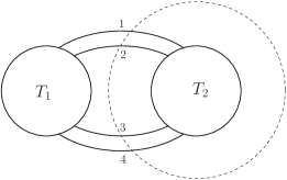
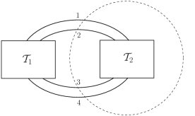
Figure 12.

In the figure, $T_{1}$ and $T_{2}$ denote some tangles and the dotted circle is the circle $C$ used in the definition of mutation. Consider the intersection points of $C$ and $D$ marked 1, 2, 3, and 4 in the figure. These points will lie on cycles in the diagram $\mathcal{D}$. Also, since $T_{1}$ and $T_{2}$ share no crossings, cutting $\mathcal{D}$ at these four points will disconnect the diagram $\mathcal{D}$. Therefore $\mathcal{D}$ can be represented schematically as in Figure 12(b), where all of the edges and other cycles are contained in the two boxes.

Since all of the cycles in $\mathcal{D}$ are closed, there exists a cycle which contains the pairs of points 1 and 2, 1 and 3, or 1 and 4.

If a cycle contains both the points 1 and 3, then since the cycles of $\mathcal{D}$ are disjoint, it must contain all of the points 1, 2, 3, and 4. This can be done in two ways: with cyclic order (1,2,3,4) or (1,4,3,2). Thus there are four cases to consider: when there is a cycle containing 1 and 2 but not 3 and 4; 1 and 4 but not 2 and 3; and the two cases when 1, 2, 3, and 4 are in the same cycle.

If a cycle contains 1 and 2 then there is also a cycle containing 3 and 4. Then, as is clear from Figure 12(a), there are vertices of the ribbon graph with cyclic ordering of the form $(1,\text{edges of }\mathcal{T}_{1},2,\text{edges of }\mathcal{T}_{2})$ and $(3,\text{edges of }\mathcal{T}_{1},4,\text{edges of }\mathcal{T}_{2})$ (or the inverse orders) and thus by cutting the discs of the ribbon graph along the interior arcs (1,2) and (3,4) we see that the ribbon graph is a 2-sum.

If a cycle contains 1 and 4 and another cycle contains 2 and 3 then in the ribbon graph there is a disc with cyclic ordering of the form $(1,\text{edges of }\mathcal{T}_{1},4,\text{edges of }\mathcal{T}_{2})$ and $(2,\text{edges of }\mathcal{T}_{1},3,\text{edges of }\mathcal{T}_{2})$ (or the inverse orders) and thus by cutting the discs of the ribbon graph along the interior arcs (1,4) and (2,3) we see that the ribbon graph is a 2-sum.

Similarly, when 1, 2, 3, and 4 are all points on the same cycle (with either order) then there is a single disc in the ribbon graph such that cutting along interior arcs (1,2) and (3,4) will separate the ribbon graph into its 2-sum components.

Finally, consider the rotation of the interior of $C$ on $D$. The corresponding effect on the diagram $\mathcal{D}$ is the same rotation of the interior of $C$. It is clear that in the ribbon graph, this corresponds to changing the way we form the 2-sum of the two ribbon graphs obtained above.

∎

References

- [1] B. Bollobás, Modern graph theory. Graduate Texts in Mathematics, 184, Springer-Verlag, New York, 1998.
- [2] B. Bollobás and O. Riordan, A polynomial for graphs on orientable surfaces, Proc. London Math. Soc. 83 (2001), 513-531.
- [3] B. Bollobás and O. Riordan, A polynomial of graphs on surfaces, Math. Ann. 323 (2002), no. 1, 81-96.
- [4] T. H. Brylawski, The Tutte Polynomial I: General Theory, in Matroid Theory and Its Applications, (ed. A Barlotti), Liguori, Naples, 1982.
- [5] T. H. Brylawski and J. G. Oxley, The Tutte polynomial and its applications, in Matroid applications (ed. N. White), 123–225, Encyclopedia Math. Appl., 40, Cambridge Univ. Press, Cambridge, 1992.
- [6] S. Chmutov and I. Pak, The Kauffman bracket of virtual links and the Bollob s-Riordan polynomial, Moscow Mathematical Journal 7 (3) (2007) 409–418, arXiv:math.GT/0609012.
- [7] S. Chmutov, J. Voltz, Thistlethwaite’s theorem for virtual links, to appear in Journal of Knot Theory and its Ramifications, 17 (2008), 1189-1198 arXiv:0704.1310 .
- [8] O. T. Dasbach, D. Futer, E. Kalfagianni, X.-S. Lin, N. W. Stoltzfus, The Jones polynomial and graphs on surfaces, Journal of Combinatorial Theory Series B, 98 (2) (2008), 384-399 arXiv:math.GT/0605571.
- [9] L. A. Goldberg and M. Jerrum, Inapproximability of the Tutte polynomial, Inform. and Comput. 206 (2008), no. 7, 908-929 arXiv:co.CC/0605140.
- [10] J. L. Gross and T. W. Tucker, Topological Graph Theory, Wiley-interscience publication, 1987.
- [11] S. Huggett, On tangles and matroids, J. Knot Theory Ramifications 14 (2005), no. 7, 919–929.
- [12] F. Jaeger, Tutte polynomials and link polynomials, Proc. Amer. Math. Soc. 103 (1988), no. 2, 647-654.
- [13] F. Jaeger, D. L. Vertigan and D. J. A. Welsh, On the computational complexity of the Jones and Tutte polynomials. Math. Proc. Cambridge Philos. Soc. 108 (1990), no. 1, 35–53.
- [14] M. Jerrum, Approximating the Tutte polynomial, Combinatorics, complexity, and chance: a tribute to Dominic Welsh, Oxford Lecture Series in Mathematics and Its Applications 34, ed. G. Grimmett and C. McDiarmid, Oxford University Press, 2007.
- [15] L. H. Kauffman, State models and the Jones polynomial, Topology 26 (1987), no. 3, 395-407.
- [16] M. Loebl and I. Moffatt, The chromatic polynomial of fatgraphs and its categorification, Advances in Math., 217 (2008) 1558-1587 arXiv:math.CO/0511557.
- [17] I. Moffatt, Knot polynomials and the Bollobás-Riordan polynomial of embedded graphs, European J. Combin., 29 (2008) 95-107 arXiv:math/0605466.
- [18] P. D. Seymour, Decomposition of regular matroids. J. Combin. Theory Ser. B 28 (1980), no. 3, 305-359.
- [19] A. D. Sokal, The multivariate Tutte polynomial (alias Potts model) for graphs and matroids, in Surveys in Combinatorics, ed. Bridget S. Webb, Cambridge University Press, 2005, pp. 173-226 arXiv:math.CO/0503607.
- [20] M. B. Thistlethwaite, A spanning tree expansion of the Jones polynomial, Topology 26 (1987), no. 3, 297-309.
- [21] L. Traldi, A dichromatic polynomial for weighted graphs and link polynomials, Proc. Amer. Math. Soc. 106 (1989), no. 1, 279-286.
- [22] D. R. Woodall, Tutte polynomial expansions for 2-separable graphs, Discrete Math. 247 (2002), 201-213.