Shape, size and robustness:
feasible regions in the parameter space of biochemical networks

Abstract

The concept of robustness of regulatory networks has been closely related to the nature of the interactions among genes, and the capability of pattern maintenance or reproducibility. Defining this robustness property is a challenging task, but mathematical models have often associated it to the volume of the space of admissible parameters. Not only the volume of the space but also its topology and geometry contain information on essential aspects of the network, including feasible pathways, switching between two parallel pathways or distinct/disconnected active regions of parameters. A general method is presented here to characterize the space of admissible parameters, by writing it as a semi-algebraic set, and then theoretically analyzing its topology and geometry, as well as volume. This method provides a more objective and complete measure of the robustness of a developmental module. As an illustration, the segment polarity gene network is analyzed.

1 Introduction

For biological networks, the concept of robustness often expresses the idea that the system’s regulatory functions should operate correctly under a variety of situations. The network should respond appropriately to various stimulii and recognize meaningful ones (either harmful or favorable), but it should also ignore small (not meaningful) variations in the environment as well as inescapable fluctuations in the abundances of biomolecules involved in the network  [1, 2, 3]. One might even speculate that if the networks malfunctions easily as a result of mutations then it has low chance of being selected by evolution. In that case one might expect a certain degree of mutational robustness [3, 4].

While it is difficult to define this robustness property in a precise form, it has been associated to the space of admissible kinetic parameters, its volume [3], and the effect of paramater perturbations on the qualitative behavior of the system [1, 2]. Some methods for parameter sensitivity have been developed  [5, 6], based essentially on derivatives of variables or fluxes with respect to the system’s parameters. The volume of the parameter space can be used as an indication of “how many” parameter combinations are possible, and these are related to the ability of the network to work under a variety of situations. For instance, parameters may range through different orders of magnitude, representing very different environments. However, size is often not a reliable measure for robustness; other quantities, such as shape, play a much more important role, as illustrated in Fig. 1. Analysis of the shape or geometry of the admissible parameter set gives an indication not only of its size, but also how far perturbations around each parameter disrupt the network. A robust biological network will admit small fluctuations in its parameters without changing its qualitative behavior. So, a robust network will be associated to a system whose parameter set has few “narrow pieces” and “sharp corners”. In such sets, reasonable parameter fluctuations may occur without leaving the set, hence maintaining the network’s qualitative behavior (compare Fig. 1 (a) and (b)). We can formalize a measure of robustness that is related to having low rate of exit from the region under random walk [4]. The rate of first exit is intrinsically connected to the geometry of the region and is particularly sensitive to narrow directions and not just the overall volume.

To illustrate the importance of parameter space geometry, and the insight it brings to understanding the network, the model of the segment polarity network developed by von Dassow and collaborators [3] will be analyzed. The segment polarity network is part of a cascade of gene families responsible for generating the segmentation of the fruit fly embryo [7]. Genes in earlier stages are transiently expressed, but the segment polarity genes maintain a stable pattern for about three hours. It has been suggested that the segment polarity genes constitute a robust developmental module, capable of autonomously reproducing the same behavior or generating the same gene expression pattern, in response to transient inputs [3, 8, 9]. This robustness would be due to the nature of interactions among genes, rather than the kinetic parameters of the reactions. The model [3] describes the interactions among the principal segment polarity genes, is continuous, and involves cell-to-cell communications and around 50 parameters which are essentially unknown. The authors of [3] explored the model by randomly choosing 240,000 parameter sets out of which about 1,192 (or $0.5\%$) sets were consistent with the generation (at steady state) of the wild type pattern. To explore the robustness of the network as a property of its interactions, Albert and Othmer [9] developed a Boolean model of the segment polarity network, a discrete logical model where each species has only two states (0 or 1; “OFF” or “ON”), but no kinetic parameters need to be defined. This Boolean model is amenable to various methods for systematic robustness analysis [10, 11, 12]. Ingolia [8] focused on the properties of the (slightly changed) model [3] in individual cells, such as bistability, and extrapolated necessary conditions on parameters to the full intercellular model.

We propose a different approach, that retains the information contained on the kinetic parameters but reduces the model to a logical form with various possible ON levels and species-dependent activation parameters. The admissible set of parameters of the model [3] is analyzed by constructing a cylindrical algebraic decomposition. Among other conclusions, our analysis completely explains the two “missing links” in von Dassow et. al. original model, namely: why the segment polarity pattern can not be recovered without the negative regulation of engrailed by Cubitus repressor protein, and why the autocatalytic wingless activation pathway vastly increases the network robustness. The present approach shows that, in contrast to volume only estimates, the topology and geometry of this set provide reliable quantitative measures of robustness of a system.

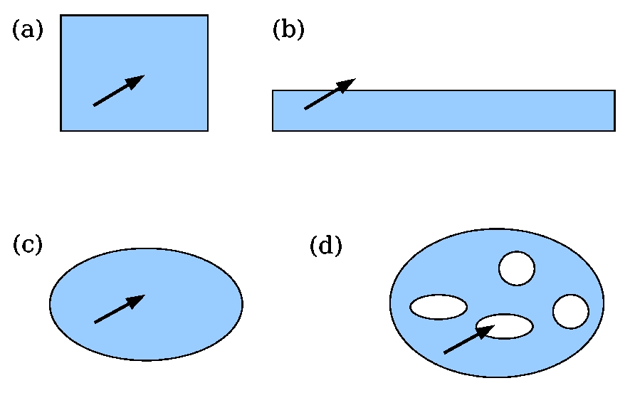
Figure 1: The role of geometry and topology in robustness. Regions (a) and (b) have the same volume, but (b) is less robust: the same perturbation leads out of the space. Regions (c) and (d) also have the same volume, but (d) is not a simply connected set, hence less robust.

2 Steady states define the feasible parameter space

Previous studies [3, 8] have tested the parameter space by randomly choosing sets of parameters and simulating the continuous model. If the corresponding trajectory reaches a steady state, and if this steady state is compatible with the experimentally observed wild type gene pattern, then the given set of parameters is said to be a “solution” to the modeling problem.

A more efficient and complete study of the parameter space can be devised, by first solving the algebraic equations of the model at steady state, and writing the steady state solutions as a function of the parameters. On the other hand, the steady state solutions are known – the set of elements representing the wild type pattern is denoted by $\mathcal{W}$ – so, one can then look for parameters that yield this pattern. Since many sets of parameters may be expected to yield the wild type pattern, this procedure provides a family of conditions defining regions of “good”or feasible parameters “$p$” for wild-type steady states $x\in\mathcal{W}$.

The von Dassow et. al. model

Before proceeding, recall that the model (Appendix B) describes the concentrations of various mRNAs and proteins in a four cell parasegment of the fly embryo, subject to periodic boundary conditions (see also Fig. 2). Here, each cell is assumed to have a square shape, with four faces (see Appendix E). We next very briefly recall the species involved. There are nine species with homogeneous concentration throughout each cell: engrailed mRNA and protein (en and EN), wingless mRNA and (internal) protein (wg and IWG), patched mRNA (ptc), cubitus mRNA, active and repressor proteins (ci, CI, and CN), and hedgehog mRNA (hh). Each of these species has a distinct concentration in each cell ($X_{i}$, $i=1,\ldots,4$). In addition, there are three other species whose concentration varies in each of the four cell faces: external wingless protein (EWG), patched protein (PTC) and hedgehog protein (HH). For each of these species, the concentration in cell $i$ at face $j$ is denoted $X_{i,j}$, $i=1,\ldots,4$, $j=1,\ldots,4$. Thus, overall there are: $n=9\times 4+3\times 4\times 4=84$ variables. Throughout the paper, the following notation will be used (prime denotes transpose):

$$X=(X_{1},X_{2},X_{3},X_{4})^{\prime},\mbox{ for }X\in\{\mbox{\it en},\mbox{EN},\mbox{\it wg},\mbox{IWG},\mbox{\it ptc},\mbox{\it ci},\mbox{CI},\mbox{CN},\mbox{\it hh}\}.$$

and

$$X=(X_{1,1},X_{1,2},X_{1,3},X_{1,4},X_{2,1},\ldots,X_{4,4})^{\prime},\mbox{ for }X\in\{\mbox{EWG},\mbox{PTC},\mbox{HH}\}.$$

The total vector of concentrations is:

$$x=(\mbox{\it en}^{\prime},\mbox{EN}^{\prime},\mbox{\it wg}^{\prime},\mbox{IWG}^{\prime},\mbox{EWG}^{\prime},\mbox{\it ptc}^{\prime},\mbox{PTC}^{\prime},\mbox{\it ci}^{\prime},\mbox{CI}^{\prime},\mbox{CN}^{\prime},\mbox{\it hh}^{\prime},\mbox{HH}^{\prime}).$$

Set of feasible parameters

In general, the problem can be formulated mathematically by writing a set of equations dependent on the vector of species concentrations ($x\in{\mathbb{R}^{n}_{\geq 0}}$) and the parameter vector ($p\in{\mathbb{R}}^{r}_{\geq 0}$), together with a set of outputs ($y\in{\mathbb{R}}^{m}_{\geq 0}$, the available gene expression levels). Introduce functions $f:{\mathbb{R}^{n}_{\geq 0}}\times{\mathbb{R}}^{r}_{\geq 0}\to{\mathbb{R}}^{n}$ and $h:{\mathbb{R}^{n}_{\geq 0}}\to{\mathcal{Y}}\subset{\mathbb{R}}^{m}_{\geq 0}$, where ${\mathbb{R}_{\geq 0}}=\{x\in{\mathbb{R}}:x_{i}\geq 0,\mbox{ for all $i$}\}$, and consider the system with outputs

$$\frac{dx}{dt} = f(x,p)$$ (1)

$$y = h(x)$$ (2)

where the function $h(x)$ could be, for instance, a vector listing the concentration of wingless, engrailed, hedgehog and cubitus, four of the segment polarity mRNAs which have been experimentally measured. Or, in other words, $y$ is “the phenotype corresponding to the genotype $x$”. The wild-type gene expression output set can be defined as:

$${\mathcal{Y}}^{\mbox{\tiny WT}}=\{y\in{\mathcal{Y}}:\ y=h(x),\ x\in\mathcal{W}\}.$$

The problem of characterizing the sets of feasible parameters is then reduced to finding all possible parameter vectors $p$ which lead the system to have an output in ${\mathcal{Y}}^{\mbox{\tiny WT}}$, at steady state. This will be the set of “good” parameters:

$$G=\{\ p\in{\mathbb{R}}^{r}_{\geq 0}:\ \exists x\mbox{ s.t. }f(x,p)=0\mbox{ and }h(x)\in{\mathcal{Y}}^{\mbox{\tiny WT}}\ \}.$$ (3)

Large Hill coefficients

A straightforward approach would be to solve the original system at steady state, obtain expressions for $x\in\mathcal{W}$ in terms of $p$, and compare these expressions to the outputs in ${\mathcal{Y}}^{\mbox{\tiny WT}}$:

$$f(x,p)=0\ \Leftrightarrow\ x=F(p)\ \ \ \mbox{and}\ \ \ F(p)\in\mathcal{W}\Leftrightarrow\ p\in G.$$

A possible drawback of this method is that explicit solutions $x=F(p)$ for the original system and then explicit formulas for $G$ may not be easy to compute. On the other hand, many of the equations in the model [3] involve terms of the form (see also Appendix B):

$$\phi(X,\kappa,\nu)=\frac{X^{\nu}}{\kappa^{\nu}+X^{\nu}},$$

meaning that the function $\phi$ is active (ON), if species $X$ is above a certain threshold $\kappa$. The exponent $\nu$, also known as the Hill coefficient, characterizes the steepness of an OFF/ON transition. For large enough exponents, this saturation function becomes very steep, and $\phi$ becomes practically insensitive to the actual value of $\nu$. As found in [13], coefficients $\nu$ must indeed be quite large for the network to achieve robustness: namely in the interval $[5.0,10.0]$. This is also the basis of the typical on/off logical interpretation of gene expression. Any such term $\phi(X,\kappa,\nu)$, for large $\nu$, may thus be replaced by a step function with two levels (0 or 1):

$$\theta(X-\kappa)=\left\{\begin{array}[]{ll}0,&X<\kappa\\ 1,&X>\kappa\ .\\ \end{array}\right.$$

Thus, when $\nu$ is large:

$$\lim_{\nu\to\infty}\,\phi(X,\kappa,\nu)=\theta(X-\kappa),\ \ \ \lim_{\nu\to\infty}\,\psi(X,\kappa,\nu)=1-\theta(X-\kappa)=\theta(\kappa-X).$$ (5)

A composite function of $\phi$ and $\psi$ also frequently appears in the continuous equations (Appendix B):

$$\phi(X_{a}\psi(X_{b}\kappa_{b},\nu_{b}),\kappa_{a},\nu_{a}).$$

This function can be simplified in terms of step functions to:

$$\theta(X_{a}\theta(\kappa_{b}-X_{b})-\kappa_{a})=\theta(X_{a}-\kappa_{a})\theta(\kappa_{b}-X_{b})$$

since

$$X_{b}>\kappa_{b}\Rightarrow\theta(\kappa_{b}-X_{b})=0\Rightarrow\theta(X_{a}\theta(\kappa_{b}-X_{b})-\kappa_{a})=\theta(-\kappa_{a})=0,$$

$$X_{b}<\kappa_{b}\Rightarrow\theta(\kappa_{b}-X_{b})=1\Rightarrow\theta(X_{a}\theta(\kappa_{b}-X_{b})-\kappa_{a})=\theta(X_{a}-\kappa_{a}).$$

As an example, consider the equation governing engrailed from the original model which can be found in [3, 13] (or in Appendix B). In this model the concentration of engrailed in cell $i$ ($\mbox{\it en}_{i}$), is positively regulated by external Wingless protein ($\mbox{EWG}_{\underline{i}}$) and negatively regulated by Cubitus repressor protein ($\mbox{CN}_{i}$) concentrations (further notation is found in Appendix A):

$$\frac{d\mbox{\it en}_{i}}{dt} = \frac{1}{H_{\mbox{\tiny\it en}}}\left(\phi(\mbox{EWG}_{\underline{i}}\psi(\mbox{CN}_{i},\kappa_{\mbox{\tiny CN}\mbox{\tiny\it en}},\nu_{\mbox{\tiny CN}\mbox{\tiny\it en}}),\kappa_{\mbox{\tiny WG}\mbox{\tiny\it en}},\nu_{\mbox{\tiny WG}\mbox{\tiny\it en}})-\mbox{\it en}_{i}\right).$$

For large exponents $\nu$, this simplifies to the equation:

$$\frac{d\mbox{\it en}_{i}}{dt} = \frac{1}{H_{\mbox{\tiny\it en}}}\left(\theta(\mbox{EWG}_{\underline{i}}-\kappa_{\mbox{\tiny WG}\mbox{\tiny\it en}})\theta(\kappa_{\mbox{\tiny CN}\mbox{\tiny\it en}}-\mbox{CN}_{i})-\mbox{\it en}_{i}\right).$$

To analyticaly study the space of feasible parameters for the segment polarity network model [3], we will thus consider that all exponents $\nu$ are large, and apply method (5) to simplify the original system of equations. The von Dassow et. al. model is then characterized by equations (32)-(43) (Appendix C). The parameters are as in [3], except $T_{i}$ and $U_{i}$, which represent the maximal values of ptc and ci (respectively), in each cell. These take values in the interval $[0,1]$ and generalize the possible ON values of ptc and ci (to be discussed later). In addition, as discussed, the system is assumed to be at steady state, in which case the gene expression pattern must satisfy:

$$\mbox{\it en}_{i}=\theta(\mbox{EWG}_{\underline{i}}-\kappa_{\mbox{\tiny WG}\mbox{\tiny\it en}})\theta(\kappa_{\mbox{\tiny CN}\mbox{\tiny\it en}}-\mbox{CN}_{i}).$$

Applying (5) and then solving the system at steady state yields the set of algebraic equations (44)-(55), which characterize the gene expression pattern of the segment polarity network according to the von Dassow et. al. model.

Maximal (ON) expression levels

While some of the species have a normalized maximal expression level (to 1), such as en or hh, other species may be more generally allowed to have any positive value (namely, ptc and ci). These maximal expression levels are also treated as parameters. When using (5) to simplify the patched equation (25) to (37), we have generalized the equation and added distinct maximal levels of expression in each cell, given by $T_{i}$ ($i=1,\ldots,4$). This allows a more accurate representation of experimental data, which shows that patched is strongly expressed in every second and fourth cells, weakly expressed in every first cell, and not expressed in every third cell (see [3] for more discussion). Thus we will consider $T_{1}<T_{2}=T_{4}$:

$$\mbox{\it ptc}_{1,2,3,4}^{\mbox{\tiny WT}}=(T_{1},T_{2},0,T_{2})^{\prime}.$$ (6)

A similar generalization was made to deal with the activation of cubitus interruptus. In von Dassow et. al. model, this is due to some external parameters $B_{i}$ (not governed by a dynamical equation), with a corresponding activity threshold $\kappa_{\mbox{\tiny B}\mbox{\tiny\it ci}}$. However, for more generality, and to allow distinct maximal levels of expression in each cell, we have replaced each of the terms $\theta(B_{i}-\kappa_{\mbox{\tiny B}\mbox{\tiny\it ci}})$ in (39) by a parameter $U_{i}$, $i=1,\ldots,4$ (51). Furthermore, in characterizing the set of feasible parameters, it will become clear that allowing distinct $U_{i}$ enlarges the space of possible parameters, by introducing the four regions $G_{\mbox{\tiny C,I}}$ to $G_{\mbox{\tiny C,IV}}$. Thus the steady state values for the cubitus mRNA are:

$$\mbox{\it ci}_{1,2,3,4}^{\mbox{\tiny WT}}=(U_{1},U_{2},0,U_{4})^{\prime}.$$ (7)

Asymmetry in cubitus expression (i.e., distinct values $U_{i}$) could be due, for instance, to some of the pair rule genes. Sloppy paired, or a combination of Runt and Factor X, regulate the transition from pair rule to segment polarity genes expression, and induce asymmetric anterior/posterior parasegment expression [14].

Finally, note that the maximal expression levels of wg are expressed in terms of the parameters $\alpha_{\mbox{\tiny CI}\mbox{\tiny\it wg}}$ and $\alpha_{\mbox{\tiny WG}\mbox{\tiny\it wg}}$. From equation (46), there are three possible combinations of the step functions, each leading to a different value for $\mbox{\it wg}_{2}$. These three possibilities are:

$$w_{\mbox{\tiny CI}}=\frac{\alpha_{\mbox{\tiny CI}\mbox{\tiny\it wg}}}{1+\alpha_{\mbox{\tiny CI}\mbox{\tiny\it wg}}},\ \ w_{\mbox{\tiny CI},\mbox{\tiny WG}}=\frac{\alpha_{\mbox{\tiny CI}\mbox{\tiny\it wg}}+\alpha_{\mbox{\tiny WG}\mbox{\tiny\it wg}}}{1+\alpha_{\mbox{\tiny CI}\mbox{\tiny\it wg}}+\alpha_{\mbox{\tiny WG}\mbox{\tiny\it wg}}},\ \ w_{\mbox{\tiny WG}}=\frac{\alpha_{\mbox{\tiny WG}\mbox{\tiny\it wg}}}{1+\alpha_{\mbox{\tiny WG}\mbox{\tiny\it wg}}},$$

and each reflects a different pathway for wingless activation. Indeed, wingless can be activated by Cubitus only (in which case the maximal amplitude is given by $w_{\mbox{\tiny CI}}$), by both Cubitus and Wingless ($w_{\mbox{\tiny CI},\mbox{\tiny WG}}$), or by Wingless only ($w_{\mbox{\tiny WG}}$).

Outputs

The next question concerns the choice of an appropriate output function. The gene expression patterns for engrailed, wingless, hedgehog, cubitus, and patched are among the most well documented, so we will consider the output function $h:{\mathbb{R}^{n}_{\geq 0}}\to{\mathbb{R}}_{\geq 0}^{20}$:

$$y=h(x)=\begin{pmatrix}h_{\mbox{\tiny\it en}}(x)\\ h_{\mbox{\tiny\it wg}}(x)\\ h_{\mbox{\tiny\it ptc}}(x)\\ h_{\mbox{\tiny\it ci}}(x)\\ h_{\mbox{\tiny\it hh}}(x)\end{pmatrix}.$$ (8)

At steady state, both en and hh are expressed in every third cell [15], which translates into

$$h_{\mbox{\tiny\it en}}(x)=(0,0,1,0)^{\prime},\ \ \ h_{\mbox{\tiny\it hh}}(x)=(0,0,1,0)^{\prime},\ \ \mbox{ for }x\in\mathcal{W}.$$ (9)

Further experimental observations show that cubitus is expressed in all but the third cell [16], and patched is strongly expressed in every second and fourth [15], but more weakly expressed in every first cell. So:

$$h_{\mbox{\tiny\it ci}}(x)=(U_{1},U_{2},0,U_{4})^{\prime},\ \ \ h_{\mbox{\tiny\it ptc}}(x)=(T_{1},T_{2},0,T_{2})^{\prime},\ \ \mbox{ for }x\in\mathcal{W}.$$ (10)

Finally, wingless (wg) is only expressed in every second cell [15], to the left of en, that is:

$$h_{\mbox{\tiny\it wg}}(x)=(0,w,0,0)^{\prime},\ \ \mbox{ for }x\in\mathcal{W}.$$ (11)

To summarize, in this example, the set of output values at steady state is:

$${\mathcal{Y}}^{\mbox{\tiny WT}}=\left\{((0,0,1,0),(0,w,0,0),(T_{1},T_{2},0,T_{2}),(U_{1},U_{2},0,U_{4}),(0,0,1,0))^{\prime}:\right.$$

$$\left.w,T_{1},T_{2},U_{1},U_{2},U_{4}>0,\ T_{1}<T_{2}\right\}.$$ (12)

The first result to be noted is that there is a unique steady state $x=x(p)\in\mathcal{W}$ for each set of parameters $p$:

Theorem 1.

Let $f$ be the function ${\mathbb{R}^{n}_{\geq 0}}\times{\mathbb{R}}^{r}_{\geq 0}\to{\mathbb{R}}^{n}$ given by (32)-(43), and $h$ be the function ${\mathbb{R}^{n}_{\geq 0}}\to{\mathcal{Y}}$ given by (8). Define $G$ as in (3). Then, there exists a function $F:G\to{\mathbb{R}^{n}_{\geq 0}}$ such that, for each $p\in{\mathbb{R}}^{r}_{\geq 0}$ and each $x\in{\mathbb{R}^{n}_{\geq 0}}$,

$$f(x,p)=0\ \ \mbox{and}\ \ h(x)\in{\mathcal{Y}}^{\mbox{\tiny WT}}\ \ \mbox{imply}\ \ x=F(p).$$

Proof.  Pick any $p\in G$, and an $x\in{\mathbb{R}^{n}_{\geq 0}}$ satisfying $f(x,p)=0$ and $h(x)\in{\mathcal{Y}}^{\mbox{\tiny WT}}$. The equations $f(x,p)=0$ can be simplified to yield (44)-(55). We must check that these equations are all consistent and admit only one solution. Since all mRNAs en, wg, ptc, ci, and hh are provided by $h(x)$, we must solve for the proteins, and then substitute these back into the equations for the mRNAs, to check consistency.

The Engrailed protein is straigthforward: $\mbox{EN}=\mbox{\it en}$. We start by solving for EWG, with $\mbox{\it wg}=(0,w,0,0)^{\prime}$ as given. First note that the matrix $M$ is diagonally dominant, by adding up the entries in any column:

$$-\left(H_{\mbox{\tiny IWG}}^{-1}+r_{\mbox{\tiny endo}}+r_{M}+2r_{LM}\right)+2r_{LM}+r_{M}+4h=-H_{\mbox{\tiny IWG}}^{-1}-r_{\mbox{\tiny endo}}\,\frac{1}{1+H_{\mbox{\tiny IWG}}r_{\mbox{\tiny exo}}}$$ (13)

which is always a negative quantity. By Geršgorin’s Theorem, all eigenvalues of $M$ are contained in the disk centered at $-d+h$ with radius $2r_{LM}+r_{M}+3h$, therefore all eigenvalues have negative real parts. Thus, the matrix $M$ is symmetric and negative definite, and since the right-hand-side vector in  (48) is also non-positive, there is a unique solution

$$\mbox{EWG}=-\frac{1}{4}\frac{r_{\mbox{\tiny exo}}}{1+H_{\mbox{\tiny IWG}}r_{\mbox{\tiny exo}}}\,M^{-1}\ \widetilde{\mbox{\it wg}}$$

which is real and positive, for each set of parameters $p$. Once we have EWG, we can immediately solve for IWG from (47).

The solution for PTC and HH can also be exactly and uniquely computed from (50) and (55), for any output $\mbox{\it ptc}=(T_{1},T_{2},0,T_{2})^{\prime}$ (this calculation is shown Appendix F).

Finally, one can now straightforwardly and uniquely compute the values of CI and CN, from (52) and (53), and the values of ci and PTC.

The last step is the substitution of EN, EWG, IWG, PTC, HH, CI and CN back into the equations for the mRNAs (44), (46), (49), (51), and (54). But, since $p\in G$, by definition we are guaranteed that these equalities are indeed satisfied.  

Missing link: engrailed regulation by Cubitus repressor

A second result from our model formulation is the explanation of a “missing link” in a first version of the model proposed by von Dassow et. al. [3]. In this first version, engrailed was regulated only by EWG, and no feasible parameter sets were found. Indeed, below (Theorem 2) we prove that, for any set of parameters, the mechanism for wingless regulation generates a strong symmetry in the steady state expression of external Wingless. This symmetry effectively prevents any asymmetry arising in en due to EWG only.

Theorem 2.

Let $w>0$ and assume $\mbox{\it wg}^{\mbox{\tiny WT}}=(0,w,0,0)^{\prime}$. Then, at steady state:

$$\mbox{EWG}_{\underline{4}}^{\mbox{\tiny WT}}<\mbox{EWG}_{\underline{1}}^{\mbox{\tiny WT}}=\mbox{EWG}_{\underline{3}}^{\mbox{\tiny WT}}<\mbox{EWG}_{\underline{2}}^{\mbox{\tiny WT}}.$$ (14)

 

The proof is based on a sequence of algebraic calculations, and is shown in Appendix E. Now, consider the steady state equation for engrailed, when no dependence on CN is assumed:

$$\mbox{\it en}_{i}^{\mbox{\tiny WT}}=\theta(\mbox{EWG}_{\underline{i}}^{\mbox{\tiny WT}}-\kappa_{\mbox{\tiny WG}\mbox{\tiny\it en}})$$

Compare to the output (9):

$$h_{\mbox{\tiny\it en}}(x)=(0,0,1,0)^{\prime}.$$

Then, from the definition of $\theta$, for consistency in our model it is necessary that:

$$\mbox{EWG}_{\underline{i}}^{\mbox{\tiny WT}}<\kappa_{\mbox{\tiny WG}\mbox{\tiny\it en}},\ \ \mbox{ for }i=1,2,4$$

$$\mbox{EWG}_{\underline{3}}^{\mbox{\tiny WT}}>\kappa_{\mbox{\tiny WG}\mbox{\tiny\it en}}.$$

However, by (14), the inequalities for $i=1,2$ and $i=3$ are incompatible. This means that, due to the symmetry in Wingless distribution, such a simple regulation of en can never lead to the segment polarity pattern. Thus engrailed requires regulation by some other factor, in this case repression by the Cubitus protein (CN), as in (44). In order to obtain repression of en in the first and second cells, one can now ask:

$$\mbox{CN}_{1}^{\mbox{\tiny WT}}>\kappa_{\mbox{\tiny CN}\mbox{\tiny\it en}},\ \ \mbox{CN}_{2}^{\mbox{\tiny WT}}>\kappa_{\mbox{\tiny CN}\mbox{\tiny\it en}}$$

$$\mbox{EWG}_{\underline{3}}^{\mbox{\tiny WT}}>\kappa_{\mbox{\tiny WG}\mbox{\tiny\it en}}\mbox{ and }\mbox{CN}_{3}^{\mbox{\tiny WT}}<\kappa_{\mbox{\tiny CN}\mbox{\tiny\it en}}$$

$$\mbox{EWG}_{\underline{4}}^{\mbox{\tiny WT}}<\kappa_{\mbox{\tiny WG}\mbox{\tiny\it en}}\mbox{ or }\mbox{CN}_{4}^{\mbox{\tiny WT}}>\kappa_{\mbox{\tiny CN}\mbox{\tiny\it en}}$$

that is, CN is responsible for repression in both the first and second cells. This means that, at steady state, CN must be expressed in both the first and second cells. This in turn requires the presence of Patched protein in both the first and second cells. On the other hand, from Appendix F, we know that a steady state $x\in\mathcal{W}$ with $h(x)\in{\mathcal{Y}}^{\mbox{\tiny WT}}$, implies $\mbox{\it ptc}_{1}^{\mbox{\tiny WT}}=\mbox{PTC}_{1}^{\mbox{\tiny WT}}$, and also $\mbox{PTC}_{2}^{\mbox{\tiny WT}}=\mbox{PTC}_{4}^{\mbox{\tiny WT}}$. This can be stated as:

Lemma 2.1.

Consider system (1) and assume that, at steady state, the output set is ${\mathcal{Y}}^{\mbox{\tiny WT}}$. Then $\mbox{\it ptc}_{1}^{\mbox{\tiny WT}}=\mbox{PTC}_{1}^{\mbox{\tiny WT}}\neq 0$. If $\mbox{\it ptc}^{\mbox{\tiny WT}}=(T_{1},T_{2},0,T_{2})^{\prime}$ with $T_{1}<T_{2}$, then $\mbox{PTC}_{1}^{\mbox{\tiny WT}}=T_{1}$ and $\mbox{PTC}_{2}^{\mbox{\tiny WT}}=\mbox{PTC}_{4}^{\mbox{\tiny WT}}>0$.  

While patched expression is typically weaker in the first than in second and fourth cells (see [3]), this shows that it is nevertheless necessary, that is, the segment polarity gene pattern obtains only when $T_{1}>0$. The discussion on CN leads to the following conclusion:

Lemma 2.2.

Consider system (1) and assume that, at steady state, the output set is ${\mathcal{Y}}^{\mbox{\tiny WT}}$. Let $\mbox{\it ptc}^{\mbox{\tiny WT}}=(T_{1},T_{2},0,T_{2})^{\prime}$ with $T_{1}<T_{2}$. Then $\mbox{PTC}_{1,2}^{\mbox{\tiny WT}}>\kappa_{\mbox{\tiny PTC}\mbox{\tiny CI}}$ and

$$\mbox{CI}_{i}^{\mbox{\tiny WT}}=U_{i}\,\frac{1}{1+H_{\mbox{\tiny CI}}C_{\mbox{\tiny CI}}},\ \ \ \mbox{CN}_{i}^{\mbox{\tiny WT}}=U_{i}\,\frac{H_{\mbox{\tiny CI}}C_{\mbox{\tiny CI}}}{1+H_{\mbox{\tiny CI}}C_{\mbox{\tiny CI}}},\ \ \ i=1,2,4,$$ (15)

and $\mbox{CI}_{3}^{\mbox{\tiny WT}}=\mbox{CN}_{3}^{\mbox{\tiny WT}}=\mbox{\it ci}_{3}^{\mbox{\tiny WT}}=0$.

Proof.  Theorem 2 and the subsequent discussion shows that $\mbox{CN}_{1,2}^{\mbox{\tiny WT}}\neq 0$ is needed. From (53), this can only be achieved by asking $\mbox{PTC}_{1,2}^{\mbox{\tiny WT}}>\kappa_{\mbox{\tiny PTC}\mbox{\tiny CI}}$. By Lemma 2.1, it also holds that $\mbox{PTC}_{2}^{\mbox{\tiny WT}}=\mbox{PTC}_{4}^{\mbox{\tiny WT}}>\kappa_{\mbox{\tiny PTC}\mbox{\tiny CI}}$. This means that both (52) and (53) can be simplified to (15), at steady state. On the third cell, $\mbox{CI}_{3}^{\mbox{\tiny WT}}=\mbox{CN}_{3}^{\mbox{\tiny WT}}=0$ because the output is zero.  

3 A cylindrical algebraic decomposition of the parameter space

The algebraic equations $f(x,p)=0$ together with $h(x)\in{\mathcal{Y}}^{\mbox{\tiny WT}}$ are a representation of the set of good parameters $G$, though not providing as yet explicit conditions on $p$. An explicit characterization of the parameters $p$ may be obtained by calculating a cylindrical algebraic decomposition (CAD) of $G$: this is a special type of representation of $G$ as a finite union of disjoint connected components. A CAD will provide a hierarchy of inequalities on $p_{1}$, $p_{2}$,$\ldots$, $p_{r}$, from which the volume of $G$, as well as its geometry and topology, may be deduced.

Computing the cylindrical algebraic decomposition of a semi-algebraic set is a complex problem, but various standard algorithms are available [17, 18]. Several software packages have been developed, for instance QEPAD [19], (based in [20]) and in Mathematica [21]. See also [22] for an overview of available software, current applications, and many other related references. Common applications of CADs include computation of the controllable or reachabable sets in hybrid systems [23]. Constructing a CAD involves the use of symbolic computation and, while various improvements have been achieved, it still is a time consuming problem. For instance, the estimated maximum time for the algorithm [17] is dominated by “$2^{2^{kN}}$”, where $N$ is the length of the input formula and $0<k\leq 8$. Fortunately, in view of these computational complexity difficulties, in the present example it is relatively easy to directly compute a CAD without using general methods, and we will do so.

For equations  (44)-(55), subject to (9)-(11), a cylindrical algebraic decomposition can be constructed in which several parameters (Table 6) are free to take any values (within physiological restrictions only). At the next level, parameters in Table 7 have constraints which depend only on those parameters given in Table 6. The last level is formed by the parameters in Table 8, whose constraints depend on parameters from both previous levels (Tables 6 and 7), thus defining a polyhedron.

Following the model of von Dassow et. al., there are two possible parallel pathways for wingless activation: either by the Cubitus interruptus protein (CI), or through auto-activation; both pathways could be simultaneously activating wingless production. Since the activation constants $\alpha_{\mbox{\tiny CI}\mbox{\tiny\it wg}}$ and $\alpha_{\mbox{\tiny WG}\mbox{\tiny\it wg}}$, are free parameters, in each of the three cases $\mbox{\it wg}_{2}^{\mbox{\tiny WT}}$ will have a different ON level (respectively, $w_{\mbox{\tiny CI}}$, $w_{\mbox{\tiny WG}}$, or $w_{\mbox{\tiny CI},\mbox{\tiny WG}}$). Computation of EWG and IWG depends on $\mbox{\it wg}_{2}^{\mbox{\tiny WT}}$, so each of these three cases must be separately analyzed for feasibility. For both pathways, exact analytic computation of $\mbox{PTC}_{i,j}$ and $\mbox{HH}_{i,j}$ ($i,j=1,\ldots,4$) is also carried out (see Appendix F). Several disconnected regions of parameters will be defined by the levels of cubitus, $U_{1,2,4}$.

Five disconnected regions

When only CI and CN regulate wingless expression, it is easy to see from (46), (11) and (15) that:

$$\left(U_{i}\frac{1}{1+H_{\mbox{\tiny CI}}C_{\mbox{\tiny CI}}}<\kappa_{\mbox{\tiny CI}\mbox{\tiny\it wg}}\ \ \mbox{ or }\ \ U_{i}\frac{H_{\mbox{\tiny CI}}C_{\mbox{\tiny CI}}}{1+H_{\mbox{\tiny CI}}C_{\mbox{\tiny CI}}}>\kappa_{\mbox{\tiny CN}\mbox{\tiny\it wg}}\right)\ \ \mbox{ and }\ \ \mbox{IWG}_{i}<\kappa_{\mbox{\tiny WG}\mbox{\tiny\it wg}}$$ (16)

for $i=1,3,4$, and

$$U_{2}\frac{1}{1+H_{\mbox{\tiny CI}}C_{\mbox{\tiny CI}}}>\kappa_{\mbox{\tiny CI}\mbox{\tiny\it wg}}\ \ \mbox{ and }\ \ U_{2}\frac{H_{\mbox{\tiny CI}}C_{\mbox{\tiny CI}}}{1+H_{\mbox{\tiny CI}}C_{\mbox{\tiny CI}}}<\kappa_{\mbox{\tiny CN}\mbox{\tiny\it wg}}\ \ \mbox{ and }\ \ \mbox{IWG}_{2}<\kappa_{\mbox{\tiny WG}\mbox{\tiny\it wg}}\ .$$ (17)

From observation of (16), (17) it is clear that the situations $U_{2}=U_{1}$ or $U_{2}=U_{4}$ are not well defined, since contradictory constraints are imposed on $\kappa_{\mbox{\tiny CI}\mbox{\tiny\it wg}}$ and $\kappa_{\mbox{\tiny CN}\mbox{\tiny\it wg}}$. So, the regions of parameters satisfying $U_{2}=U_{1}$ or $U_{2}=U_{4}$ are not feasible. This divides the set $G$ into at least four disconnected components, divided by the hyperplanes $U_{2}=U_{1}$ or $U_{2}=U_{4}$ ($G_{\mbox{\tiny C,I}}$, $G_{\mbox{\tiny C,II}}$, $G_{\mbox{\tiny C,III}}$, and $G_{\mbox{\tiny C,IV}}$ in Fig. 3). A similar argument holds for the case when both pathways contribute to activation of wingless on the second cell. The four disconnected regions of parameters are identified in Table 8.

Finally, the third case (auto-activation pathway only), introduces a fifth component of $G$ ($G_{\mbox{\tiny Auto}}$), which must be disconnected from either of the previous four components. This is clear, by contrasting the necessary conditions in the second cell for either case (compare to (17)):

$$\left(U_{2}\frac{1}{1+H_{\mbox{\tiny CI}}C_{\mbox{\tiny CI}}}<\kappa_{\mbox{\tiny CI}\mbox{\tiny\it wg}}\ \ \mbox{ or }\ \ U_{2}\frac{H_{\mbox{\tiny CI}}C_{\mbox{\tiny CI}}}{1+H_{\mbox{\tiny CI}}C_{\mbox{\tiny CI}}}>\kappa_{\mbox{\tiny CN}\mbox{\tiny\it wg}}\right)\ \ \mbox{ and }\ \ \mbox{IWG}_{2}>\kappa_{\mbox{\tiny WG}\mbox{\tiny\it wg}}.$$ (18)

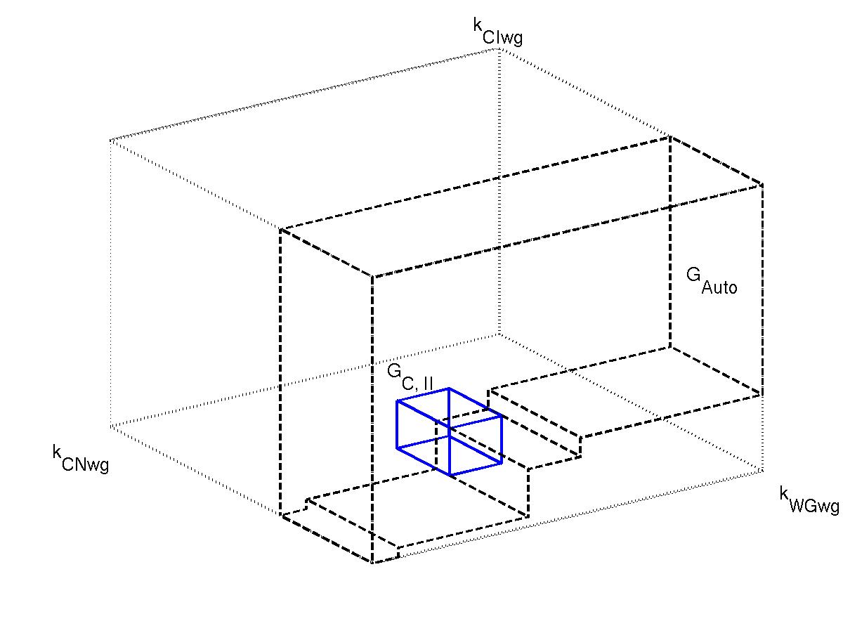
Figure 4: An example of regions $G_{\mbox{\tiny C,II}}$ (solid line rectangle) and $G_{\mbox{\tiny Auto}}$ (dashed line polyhedron). This is the projection on the space $(\kappa_{\mbox{\tiny CI}\mbox{\tiny\it wg}},(\kappa_{\mbox{\tiny CN}\mbox{\tiny\it wg}},(\kappa_{\mbox{\tiny WG}\mbox{\tiny\it wg}})$, of the fibre over the point represented by “$*$” in Fig. 3. This points corresponds to choosing values for $(U_{1},U_{2},U_{4})$ in region $G_{\mbox{\tiny C,II}}$.

The five disconnected components are thus first defined by $U_{1}$, $U_{2}$, and $U_{4}$, and then by $\kappa_{\mbox{\tiny CI}\mbox{\tiny\it wg}}$ and $\kappa_{\mbox{\tiny CN}\mbox{\tiny\it wg}}$. The projection on the ($\kappa_{\mbox{\tiny CI}\mbox{\tiny\it wg}}$,$\kappa_{\mbox{\tiny CN}\mbox{\tiny\it wg}}$,$\kappa_{\mbox{\tiny WG}\mbox{\tiny\it wg}}$)-dimensions compares two of these components ($G_{\mbox{\tiny C,II}}$ and $G_{\mbox{\tiny Auto}}$), both polyhedrons (Fig. 4).

The cylindrical algebraic decomposition is shown in detail in Appendix G, and summarized in Tables 6,7,8. Each of the five components, $G_{\gamma}\in\{G_{\mbox{\tiny C,I}},G_{\mbox{\tiny C,II}},G_{\mbox{\tiny C,III}},G_{\mbox{\tiny C,IV}},G_{\mbox{\tiny Auto}}\}$ is thus described by a hierarchy of sets of the form:

$$S_{1,\gamma} = (a_{\gamma},b_{\gamma})\subset{\mathbb{R}}$$

$$S_{i,\gamma} = \{(x,x_{i})\in{\mathbb{R}}^{i}:\ x\in S_{i-1,\gamma},\ \alpha_{i,\gamma}(x)<x_{i}<\beta_{i,\gamma}(x)\}\subset{\mathbb{R}}^{i}$$ (19)

for $i=2,\ldots,N$, where $\alpha_{i,\gamma},\beta_{i,\gamma}:S_{i-1,\gamma}\to{\mathbb{R}}_{>0}$ and $S_{N,\gamma}=G_{\gamma}$. It can be shown that each $G_{\gamma}$ is in fact topologically equivalent to the unitary open hypercube, and hence topologically trivial.

Theorem 3.

For each $G_{\gamma}$, the set $S_{N}=S_{N,\gamma}$, as obtained from (3), is homeomorphic to $(0,1)^{N}$.

Proof.  Pick any $G_{\gamma}$, and drop the subscript $\gamma$, for simplicity of notation. To argue by induction, note that the set $S_{1}$ is clearly homeomorphic to $(0,1)$. For $i\geq 2$, assume that $S_{i-1}$ is homeomorphic to $(0,1)^{i-1}$. Next, define the following continuous function:

$$\varphi_{i}:S_{i-1}\times(0,1)\to S_{i-1}\times{\mathbb{R}},\ \ \ \varphi_{i}(x,t)=(x,f_{i}(x)+t\,(g_{i}(x)-f_{i}(x))).$$

For each fixed $x$, $\alpha_{i}(x)<\alpha_{i}(x)+t\,(\beta_{i}(x)-\alpha_{i}(x))<\beta_{i}(x)$ for all $t\in(0,1)$. Therefore, $\varphi_{i}$ maps into $S_{i}$. On the other hand, $\varphi_{i}$ has an inverse function defined on $S_{i}$ and continuous, given by:

$$\varphi_{i}^{-1}:S_{i}\to S_{i-1}\times(0,1),\ \ \ \varphi_{i}^{-1}(x,y)=\left(x,\frac{y-\alpha_{i}(x)}{\beta_{i}(x)-\alpha_{i}(x)}\right).$$

So $S_{i}$ is homeomorphic to $S_{i-1}\times(0,1)$, and therefore, by inductive hypothesis, to $(0,1)^{i}$, as we wanted to show.  

Relative volume and the second missing link

Once the parameter set $G$ is characterized by writing intervals for the various parameters in the form  (3), it is very easy to compute the (relative) volumes of the disconnected components. Note that in each component only the intervals for $U_{1}$, $U_{2}$, $U_{4}$, and $\kappa_{\mbox{\tiny CN}\mbox{\tiny\it en}}$, $\kappa_{\mbox{\tiny WG}\mbox{\tiny\it en}}$, $\kappa_{\mbox{\tiny CI}\mbox{\tiny\it wg}}$, $\kappa_{\mbox{\tiny CN}\mbox{\tiny\it wg}}$, $\kappa_{\mbox{\tiny WG}\mbox{\tiny\it wg}}$ vary; constraints on the remaining parameters are common to all components. Following a Monte Carlo approach, the parameters in Tables 6,7 are chosen first, and then $\kappa_{\mbox{\tiny CI}\mbox{\tiny\it wg}}$, $\kappa_{\mbox{\tiny CN}\mbox{\tiny\it wg}}$, $\kappa_{\mbox{\tiny WG}\mbox{\tiny\it wg}}$ from the unitary cube (all parameters are randomly chosen from uniform distributions in the given intervals). It is next checked whether the parameter set falls in any of the components $G_{\mbox{\tiny C,I}}$, $G_{\mbox{\tiny C,II}}$, $G_{\mbox{\tiny C,III}}$, $G_{\mbox{\tiny C,IV}}$, $G_{\mbox{\tiny Auto}}$, or outside $G$. This method provides an estimate of the volumes of each disconnected component, when projected into the ($\kappa_{\mbox{\tiny CN}\mbox{\tiny\it en}}$,$\kappa_{\mbox{\tiny WG}\mbox{\tiny\it en}}$,$\kappa_{\mbox{\tiny CI}\mbox{\tiny\it wg}}$,$\kappa_{\mbox{\tiny CN}\mbox{\tiny\it wg}}$,$\kappa_{\mbox{\tiny WG}\mbox{\tiny\it wg}}$) dimensions, as the fraction of parameter sets that fall into each component. The volume of this 5-dimensional cube occupied by feasible parameter sets is only about 0.7%. As is illustrated by the polyhedrons in Fig. 4, component $G_{\mbox{\tiny Auto}}$ is much larger than the others – approximately 40 to 270 times larger.

Table 1: Relative volumes of the five disconnected components. In component $G_{\mbox{\tiny Auto}}$, only auto-activation leads to wingless expression. In components $G_{\mbox{\tiny C,I}}$, $G_{\mbox{\tiny C,II}}$, $G_{\mbox{\tiny C,III}}$, and $G_{\mbox{\tiny C,IV}}$, CI always activates wingless expression. Total number of parameter sets generated: $1\times 10^{7}$. Number of feasible parameter sets: 70026.

Component	Volume
$G_{\mbox{\tiny C,I}}$	$1.6\times 10^{-4}$
$G_{\mbox{\tiny C,II}}$	$0.25\times 10^{-4}$
$G_{\mbox{\tiny C,III}}$	$0.86\times 10^{-4}$
$G_{\mbox{\tiny C,IV}}$	$0.46\times 10^{-4}$
$G_{\mbox{\tiny Auto}}$	$67\times 10^{-4}$

The large difference observed between $G_{\mbox{\tiny C,I}}$-$G_{\mbox{\tiny C,IV}}$ and $G_{\mbox{\tiny Auto}}$ explains the second “missing link” in the first version of von Dassow et. al. model, namely the wingless autocatalytic activation. Note that the presence of this link greatly increases the total volume of the feasible parameter space: in fact the region $G_{\mbox{\tiny Auto}}$ is 95% of the total volume.

Parameter tendencies

As described above, the parameter space for the segment polarity network can be described by a CAD, a hierarchy of inequalities on the parameters where an interval is explicitly given for each parameter. At the base of this hierarchy, there is a first group of parameters whose intervals correspond simply to physiological values, as in Table 6. The intervals for the remaining parameters have bounds which depend on the parameters in the first group (Tables 7 and 8). In any case, one may ask how the parameters are distributed in their intervals, whether each parameter $p_{i}$ is more likely to attain high or low values more frequently, or whether a “tendency” for each parameter $p_{i}$ be identified. An answer to this question is obtained by randomly generating parameters in the full parameter space $G$, and computing the distribution of each parameter. Taking all the parameter sets generated to compute the relative volumes of the five disconnected components of $G$, and computing a histogram for each parameter, the result shown on Fig. 5 is obtained. As expected, many parameters have a uniform distribution, as their values do not influence the final outcome of the network in any particular way (for instance, most half-lives). Other parameters exhibit a marked tendency for higher (e.g., $\kappa_{\mbox{\tiny CN}\mbox{\tiny\it ptc}}$), medium (e.g., $\kappa_{\mbox{\tiny WG}\mbox{\tiny\it wg}}$) or lower (e.g., $\kappa_{\mbox{\tiny CI}\mbox{\tiny\it ptc}}$) values. All the parameters that exhibit a marked tendency are listed in Table 2, and classified according to their function in the network: for instance, $\kappa_{\mbox{\tiny CN}\mbox{\tiny\it ptc}}$ represents the repression of ptc by CN, and therefore, high values of $\kappa_{\mbox{\tiny CN}\mbox{\tiny\it ptc}}$ correspond to a weak repression.

A very similar analysis was performed by von Dassow and Odell [13], who also plotted the distribution of their family of feasible parameters to determine possible constraints for each parameter. Overall, our results agree very well with those of von Dassow and Odell: most tendencies found by these authors (see Fig. 6 and Table 1 of [13]) are confirmed by our parameter space analysis. There are only five exceptions, where our analysis showed no tendency (compare columns 3 and 4 of Table 2), suggesting that these five parameters can, in fact, take values in a larger set, implying that the parameter space is larger than estimated in [13]. From these exceptions, $\kappa_{\mbox{\tiny EN}\mbox{\tiny\it ci}}$, $\kappa_{\mbox{\tiny EN}\mbox{\tiny\it hh}}$, $\kappa_{\mbox{\tiny CN}\mbox{\tiny\it hh}}$, and $r_{\mbox{\tiny endo}}$${}_{\mbox{\tiny WG}}$ all belong to the group of parameters which can be freely chosen. The other parameter is $\kappa_{\mbox{\tiny CI}\mbox{\tiny\it wg}}$, which depends on the disconnected regions, and again our analysis shows that this pair has no preferred tendency.

A more detailed examination of the conditions on $\kappa_{\mbox{\tiny CI}\mbox{\tiny\it wg}}$ and $\kappa_{\mbox{\tiny CN}\mbox{\tiny\it wg}}$ turns out to be very illuminating. First, note that $\kappa_{\mbox{\tiny CI}\mbox{\tiny\it wg}}$ and $\kappa_{\mbox{\tiny CN}\mbox{\tiny\it wg}}$ define the five components, in the sense that distinct intervals for these two parameters are given in each component. Thus, it may be expected that the distribution of these parameters varies in each region (Table 3). Indeed, by plotting the histograms for $\kappa_{\mbox{\tiny CI}\mbox{\tiny\it wg}}$ and $\kappa_{\mbox{\tiny CN}\mbox{\tiny\it wg}}$ for each region alone, we note that these show a marked tendency in components $G_{\mbox{\tiny C,I}}-G_{\mbox{\tiny C,IV}}$, for low $\kappa_{\mbox{\tiny CI}\mbox{\tiny\it wg}}$ and high $\kappa_{\mbox{\tiny CN}\mbox{\tiny\it wg}}$. In contrast, the distributions of $\kappa_{\mbox{\tiny CI}\mbox{\tiny\it wg}}$ and $\kappa_{\mbox{\tiny CN}\mbox{\tiny\it wg}}$ for region $G_{\mbox{\tiny Auto}}$ alone show an opposite tendency. This is consistent with the fact that the volume of $G_{\mbox{\tiny Auto}}$ is about 95% of $G$ and, therefore, it dominates the overall tendency. Note also that, in the four components $G_{\mbox{\tiny C,I}}-G_{\mbox{\tiny C,IV}}$, it always holds that $\kappa_{\mbox{\tiny CI}\mbox{\tiny\it wg}}<\kappa_{\mbox{\tiny CN}\mbox{\tiny\it wg}}$, clearly in agreement with the tendency observed for our parameter sets. In component $G_{\mbox{\tiny Auto}}$, the parameters $\kappa_{\mbox{\tiny CI}\mbox{\tiny\it wg}}$ and $\kappa_{\mbox{\tiny CN}\mbox{\tiny\it wg}}$ must satisfy constraints that contradict those of $G_{\mbox{\tiny C,I}}-G_{\mbox{\tiny C,IV}}$, but not necessarily exactly opposite constraints (see Table 8). Thus more freedom results for the choice of $\kappa_{\mbox{\tiny CI}\mbox{\tiny\it wg}}$ and $\kappa_{\mbox{\tiny CN}\mbox{\tiny\it wg}}$ in $G_{\mbox{\tiny Auto}}$. The tendency of $\kappa_{\mbox{\tiny CI}\mbox{\tiny\it wg}}$ and $\kappa_{\mbox{\tiny CN}\mbox{\tiny\it wg}}$ in $G_{\mbox{\tiny C,I}}-G_{\mbox{\tiny C,IV}}$ is, however, the opposite of that observed by von Dassow and Odell, a fact that can be explained once again by the “second missing link”. Indeed, since all feasible parameter sets in [3, 13] were found only after adding the autocatalytic wingless activation link, it can be inferred that those parameters belong to region $G_{\mbox{\tiny Auto}}$. We conclude that the parameter space is larger than estimated by von Dassow and Odell.

Table 2: Comparison between the constraints identified by von Dassow and Odell [13], and the exact constraints given by the five regions defined above. Total number of parameters generated in $G$: 70026.

Parameter	Description	Tendency	Tendency
		([13], Table 1)	(within $G$)
$\kappa_{\mbox{\tiny WG}\mbox{\tiny\it en}}$	WG activation of en	Moderate	Moderate
$\kappa_{\mbox{\tiny CN}\mbox{\tiny\it en}}$	CN repression of en	Strong	Strong
$\kappa_{\mbox{\tiny WG}\mbox{\tiny\it wg}}$	WG autoactivation	Moderate	Moderate
$\kappa_{\mbox{\tiny CI}\mbox{\tiny\it wg}}$	CI activation of wg	Weak	—
$\kappa_{\mbox{\tiny CN}\mbox{\tiny\it wg}}$	CN repression of wg	Strong	Strong
$\kappa_{\mbox{\tiny CI}\mbox{\tiny\it ptc}}$	CI activation of ptc	Strong	Strong
$\kappa_{\mbox{\tiny CN}\mbox{\tiny\it ptc}}$	CN repression of ptc	Weak	Weak
$\kappa_{\mbox{\tiny EN}\mbox{\tiny\it ci}}$	EN repression of ci	Moderate	—
$\kappa_{\mbox{\tiny PTC}\mbox{\tiny CI}}$	PTC stimulation of CI cleavage	Strong	Strong
$\kappa_{\mbox{\tiny EN}\mbox{\tiny\it hh}}$	EN activation of hh	Weak	—
$\kappa_{\mbox{\tiny CN}\mbox{\tiny\it hh}}$	CN repression of hh	Strong	—
$C_{\mbox{\tiny CI}}$	Maximal cleavage rate of CI	Rapid	Rapid
$H_{\mbox{\tiny IWG}}$	Half-life of intracellular WG	Short	Short
$r_{\mbox{\tiny endo}}$${}_{\mbox{\tiny WG}}$	Rate of WG endocytosis	Slow	—
$r_{\mbox{\tiny exo}}$${}_{\mbox{\tiny WG}}$	Rate of WG exocytosis	Moderately slow	Moderately fast
$r_{\mbox{\tiny Mxfer}\mbox{\tiny WG}}$	Rate of WG cell-to-cell exchange	Slow	Slow
$\alpha_{\mbox{\tiny WG}\mbox{\tiny\it wg}}$	Maximal WG autocatalytic rate	—	Moderately rapid

Table 3: Influence of the autocatalytic WG activation link in the parameter distribution.

Parameter	Tendency	Tendency	Tendency
	([13], Table 1)	$G_{\mbox{\tiny Auto}}$	$G_{\mbox{\tiny C,I}},G_{\mbox{\tiny C,II}},G_{\mbox{\tiny C,II}},G_{\mbox{\tiny C,IV}}$
		($\mbox{WG}\rightarrow\mbox{\it wg}$)	($\mbox{WG}\nrightarrow\mbox{\it wg}$)
$\kappa_{\mbox{\tiny CI}\mbox{\tiny\it wg}}$	Weak	Weak	Strong
$\kappa_{\mbox{\tiny CN}\mbox{\tiny\it wg}}$	Strong	(Moderately) Strong	Weak

4 Geometry and robustness

The volume estimates for the parameter space regions give an idea of “how many” parameter combinations are possible. But volume alone is often not a reliable measure for robustness, as illustrated in Fig. 1. The shape or geometry of the parameter space regions also shows how far perturbations around each parameter will disrupt the network. Thus, parameter regions exhibiting “narrow” pieces or “sharp” corners indicate a lower level of robustness in the network. One way to explore the shape of a given multi-dimensional set is to consider a random point ($p^{0}$) and follow a random walk in space ($p^{k}=p^{k-1}+dp^{k}$, $k=1,2,\ldots,$), where each step has the same absolute length ($|{dp^{k}}|=a_{0}$), but a random direction. Then record the number of steps needed for the point to exit the given set. Repeating this procedure for many points in the set, the probability that a point leaves the set after $t$ steps can be computed.

The random walk could be interpreted as parameter changes due to evolution, and the probability of exiting after $t$ steps represents the probability that the network is no longer capable of correctly performing its function (for instance, when a lethal mutation occurs). Studying the first exit problem is the natural thing to do in certain evolutionary models. Suppose we consider a fitness landscape on the parameter space where the functioning regions have a fixed high fitness and every other region has zero fitness. If we consider a space of alleles to be nearly continuous and model the effect of mutation as diffusion in this space, as is often done in the adaptive dynamics literature [24], we find that we need to compute the mutation load, namely the rate of death from exiting the high fitness region. This idea was previously used in the context of transcriptional networks [4].

To explore the shape of the regions $G_{\mbox{\tiny C,I}}$ to $G_{\mbox{\tiny Auto}}$, Algorithm I uses a random walk in the parameter space, and checks “exit times” as well as the “failed parameters”.

Algorithm I

• Pick a positive number $a_{0}$ to be the constant magnitude of the random walk step.

• Repeat points 1-4 (run $q$), $Q$ times.

• Step $0$: generate a point $p^{0}=(p_{1}^{0},\ldots,p_{m}^{0})^{\prime}$ at random in the parameter region $G_{\gamma}$;

• Step $k-1/2$, $k\geq 1$: generate a random perturbation $dp^{k}\in[-a_{0},a_{0}]^{m}$, such that $|{dp^{k}}|=a_{0}$;

• Step $k$, $k\geq 1$: check if $p^{k}=p^{k-1}+dp^{k}$ is still in $G_{\gamma}$;

• Check. The random walk exits the parameter region at time $t$ if $p^{k}\in G_{\gamma}$ for $k<t$ but $p^{t}\notin G_{\gamma}$.
  Let $p_{j_{1}}^{t},\ldots,p_{j_{J}}^{t}$ be parameters that fail to satisfy the hierarchy of conditions which defines $G_{\gamma}$.
  Update the exit times vector: exit($q$)=$t$.
  Update the failed parameters vector: failpar($q$)=$[j_{1},\ldots,j_{J}]$.
  

To interpret the numerical results obtained with Algorithm I, define the probability that a mutation takes place in the first $t$ steps by:

$$P_{\mbox{\tiny mut}}(t)=\frac{1}{Q}\mbox{ card}(I_{t}),\ \ \ I_{t}=\{q\in{\mathbb{N}}:\texttt{exit($q$)}\leq t\},$$

where card($\cdot$) denotes the cardinality of a set. Algorithm I was applied to each component of the feasible parameter space of the segment polarity network, with $a_{0}=1\times 10^{-3}$ and $Q=4000$. Two striking facts are revealed. First, with a significant probability, fluctuations in the parameters will drive the system from the operating regions $G_{\mbox{\tiny C,I}}$, $G_{\mbox{\tiny C,II}}$, $G_{\mbox{\tiny C,III}}$, or $G_{\mbox{\tiny C,IV}}$, to the region $G_{\mbox{\tiny Auto}}$ and, conversely, switching was also observed from $G_{\mbox{\tiny Auto}}$ to the other four (see the switching column in Table 4). Recalling the difference between $G_{\mbox{\tiny Auto}}$ and the other four components, this means that, in a significant number cases, the network responds to perturbations by switching to an alternative biological pathway, rather than break down. A second fact is that only a very small number of parameters (six out of 39, namely $\kappa_{\mbox{\tiny CN}\mbox{\tiny\it en}}$, $\kappa_{\mbox{\tiny WG}\mbox{\tiny\it en}}$, $\kappa_{\mbox{\tiny CI}\mbox{\tiny\it ptc}}$, $\kappa_{\mbox{\tiny PTC}\mbox{\tiny CI}}$, $\kappa_{\mbox{\tiny CI}\mbox{\tiny\it wg}}$, $\kappa_{\mbox{\tiny CN}\mbox{\tiny\it wg}}$) are responsible for above 90% of network failures or mutations. The percentage of cases where each of these parameters failed is shown in Table 4.

Table 4: Fragile parameters.

$G_{\gamma}$	% switching	% failed	% failed	% failed	% failed	% failed	% failed
		$\kappa_{\mbox{\tiny CN}\mbox{\tiny\it en}}$	$\kappa_{\mbox{\tiny WG}\mbox{\tiny\it en}}$	$\kappa_{\mbox{\tiny CI}\mbox{\tiny\it ptc}}$	$\kappa_{\mbox{\tiny PTC}\mbox{\tiny CI}}$	$\kappa_{\mbox{\tiny CI}\mbox{\tiny\it wg}}$	$\kappa_{\mbox{\tiny CN}\mbox{\tiny\it wg}}$
$G_{\mbox{\tiny C,I}}$	$1.21\%$ (to $G_{\mbox{\tiny Auto}}$)	$5.4\%$	$6.3\%$	$20.0\%$	$4.4$	$50.8\%$	$5.6\%$
$G_{\mbox{\tiny C,II}}$	$0.88\%$ (to $G_{\mbox{\tiny Auto}}$)	$4.7\%$	$5.6\%$	$17.2\%$	$4.3$	$40.0\%$	$18.7\%$
$G_{\mbox{\tiny C,III}}$	$1.50\%$ (to $G_{\mbox{\tiny Auto}}$)	$6.2\%$	$5.2\%$	$30.8\%$	$4.1$	$35.0\%$	$11.5\%$
$G_{\mbox{\tiny C,IV}}$	$1.16\%$ (to $G_{\mbox{\tiny Auto}}$)	$4.9\%$	$5.3\%$	$16.8\%$	$5.0$	$40.1\%$	$18.9\%$
$G_{\mbox{\tiny Auto}}$	$0.02\%$ (to $G_{\mbox{\tiny C,I}}$-$G_{\mbox{\tiny C,IV}}$)	$8.5\%$	$5.7\%$	$21.2\%$	$4.8$	$31.4\%$	$18.8\%$

Calculating the distribution function $P_{\mbox{\tiny mut}}$ shows that the probability of mutation increases very rapidly for small times, in all five components (see Fig. 6) – this indicates a low robustness of the network, because it is very likely that a very small number of fluctuations leads out of the feasible parameter space. To compare the results for the five components, we computed some quantities of interest. A possible indicator of robustness is $T_{1/2}$, defined as the time for which there is a 50% chance that the system has already suffered a mutation. Low $T_{1/2}$ indicates a system which has a low robustness to perturbations. Another indicator is $P_{\mbox{\tiny mut}}(10)$, which gives the probability that the system has been disrupted after only 10 perturbation steps. Similarly, the values $P_{\mbox{\tiny mut}}(100)$, $P_{\mbox{\tiny mut}}(1000)$, and $P_{\mbox{\tiny mut}}(10000)$ are also shown for comparison. The computed values are summarized in Table 5.

Table 5: Indicators of robustness.

$G_{\gamma}$	$T_{1/2}$	$P_{\mbox{\tiny mut}}(10)$	$P_{\mbox{\tiny mut}}(100)$	$P_{\mbox{\tiny mut}}(1000)$	$P_{\mbox{\tiny mut}}(10000)$
$G_{\mbox{\tiny C,I}}$	$18$	$0.40$	$0.74$	$0.94$	$0.99$
$G_{\mbox{\tiny C,II}}$	$23$	$0.37$	$0.72$	$0.94$	$0.99$
$G_{\mbox{\tiny C,III}}$	$19$	$0.40$	$0.72$	$0.93$	$0.99$
$G_{\mbox{\tiny C,IV}}$	$23$	$0.37$	$0.73$	$0.94$	$0.99$
$G_{\mbox{\tiny Auto}}$	$309$	$0.30$	$0.41$	$0.61$	$0.88$

Comparison of the values for $T_{1/2}$ and $P_{\mbox{\tiny mut}}(10^{d})$ ($d=1,\ldots,4$) in the five regions, shows clearly that the components $G_{\mbox{\tiny C,I}}$ to $G_{\mbox{\tiny C,IV}}$ result in a less robust network, while $G_{\mbox{\tiny Auto}}$ exhibits a much higher level of robustness. Furthermore, there is a non-negligible probability ($\approx 1\%$) that the network switches from the other components to $G_{\mbox{\tiny Auto}}$ instead of breaking down, thus contributing to the robustness level of this component. Distinguishing the levels of robustness among the four regions $G_{\mbox{\tiny C,I}}$ to $G_{\mbox{\tiny C,IV}}$ is not straightforward, since the indicators $P_{\mbox{\tiny mut}}(10^{d})$ and $T_{1/2}$ are very similar.

As noted above, only six out of 39 parameters are responsible for over 90% of failures. Curiously, two of these parameters satisfies constraints which are in fact independent of the regions ($\kappa_{\mbox{\tiny CI}\mbox{\tiny\it ptc}}$ and $\kappa_{\mbox{\tiny PTC}\mbox{\tiny CI}}$, see Table 7). So, the numerical results clearly show that the parameter space is very narrow in the directions defined by $\kappa_{\mbox{\tiny CI}\mbox{\tiny\it ptc}}$ and $\kappa_{\mbox{\tiny PTC}\mbox{\tiny CI}}$. The other critical directions are defined by $\kappa_{\mbox{\tiny CI}\mbox{\tiny\it wg}}$ and $\kappa_{\mbox{\tiny CN}\mbox{\tiny\it wg}}$, and $\kappa_{\mbox{\tiny CN}\mbox{\tiny\it en}}$ and $\kappa_{\mbox{\tiny WG}\mbox{\tiny\it en}}$, which satisfy different conditions in each of the five parameter regions (Table 8). Together with common parameter $\kappa_{\mbox{\tiny CI}\mbox{\tiny\it ptc}}$, the parameters that regulate activation and inhibition of wingless by Cubitus proteins ($\kappa_{\mbox{\tiny CI}\mbox{\tiny\it wg}}$ and $\kappa_{\mbox{\tiny CN}\mbox{\tiny\it wg}}$) are the most critical.

The main conclusion from Algorithm I clearly follows the preliminary estimates of the relative volumes (compare Tables 1 and 5, both concluding that $G_{\mbox{\tiny Auto}}$ is more robust than the other four components). But the geometry analysis reveals three new fundamental results: (i) the system increases its robustness to environment perturbations by switching to an alternative biological pathway. The switching event may be from a “small” to a “large” region but also, more remarkably, from a “large” to a “small”; (ii) the lack of robustness is due not only to small sized regions, but in part to critical parameters ($\kappa_{\mbox{\tiny CI}\mbox{\tiny\it ptc}}$ and $\kappa_{\mbox{\tiny PTC}\mbox{\tiny CI}}$), which define directions along which the parameter space is globally very narrow; (iii) the volume alone is not a reliable measure of robustness, since volume (Table 1) and the indicator $T_{1/2}$ provide different robustness classifications for components $G_{\mbox{\tiny C,I}}$ to $G_{\mbox{\tiny C,IV}}$. For instance, the volume of $G_{\mbox{\tiny C,II}}$ is apparently the smallest (an indicator of low robustness), but $T_{1/2}$ is the largest (an indicator of high robustness), suggesting that the shape of the region does plays an important role. In contrast, the numbers $P_{\mbox{\tiny mut}}(10^{d})$ are very similar, suggesting that robustness levels of $G_{\mbox{\tiny C,I}}$ to $G_{\mbox{\tiny C,IV}}$ are in fact very similar. However, it should be noted that neither volume nor $T_{1/2}$ provide conclusive information on the relative levels of robustness of $G_{\mbox{\tiny C,I}}$ to $G_{\mbox{\tiny C,IV}}$. In particular, note that $T_{1/2}$ depends on the magnitude of the random walk step - other numerical experiments were performed with different $a_{0}$ values (not shown), and the comparison results are unchanged.

5 Discussion and conclusions

Analysis of the feasible parameter set, by estimating its volume, identifying connected components, and its geometric properties are valuable tools for establishing and quantifying robustness in regulatory networks. The concept of robustness, in the sense that the system’s regulatory functions should operate correctly under a variety of situations, is closely related to the parameter space and the effect of parameter perturbations. In this context, our analysis suggests that the segment polarity network is vulnerable to perturbations in its parameters. Indeed, the first striking result from our analysis is that the feasible parameter space is composed of five disconnected components. An implication of this topological characterization is a diminished capacity of the network to respond well to environmental perturbations. Random fluctuations will often drive the system to a set of parameters outside any feasible region, and thus lead to a break down of the network or a different phenotype. Indeed, as the results of Algorithm I show, sucessive random perturbations to the parameters will drive the system out of the feasible parameter set, with a large probability. For instance, if parameters are randomly perturbed for up to 10 times, each of magnitude $1\times 10^{-3}$ in any direction, there is a 30% probability that the system will fail to operate correctly (see Table 5, column $P_{\mbox{\tiny mut}}(10)$). On the other hand, it is possible that a series of fluctuations in the environment may drive the system to adopt an alternative biochemical pathway, and thus “jump” from one feasible component to another (with probability 1%, see Table 4).

As the group of most fragile parameters suggest, the Cubitus-wingless interactions are at the basis of the appearance of disconnected regions of parameters. Dis-connectivity in the space of parameters can be traced in large part to an incompatibility of Cubitus repression functions in the second cell: $\mbox{CN}_{2}$ should be present to repress engrailed expression, but should be absent to enhance $\mbox{CI}_{2}$ activation of wingless. To increase the network’s robustness to environmental fluctuations, the segment polarity model should account for engrailed regulation by other factor than Cubitus. One possibility is to include regulation by pair-rule gene products, such as Sloppy paired, as explored both in [9] and  [8]. An external factor, again possibly from the pair-rule genes, will also play a major role in establishing asymmetry in the cubitus levels ($U_{i}$). These contribute to a larger admissible parameter space, and together with an improved engrailed regulation, will greatly enhance robustness of the segment polarity network in maintaining its pattern. An extension of the current analysis including the regulation by Sloppy paired is currently in preparation by A. Dayarian at one of our labs [26].

Both the volume estimates and the probability of failure or mutation ($P_{\mbox{\tiny mut}}$) in each component indicate that $G_{\mbox{\tiny Auto}}$ is the most robust parameter region, while $G_{\mbox{\tiny C,I}}$, $G_{\mbox{\tiny C,II}}$, $G_{\mbox{\tiny C,III}}$ and $G_{\mbox{\tiny C,IV}}$ are less robust regions, all at the same level. However, volume is not a reliable indicator of robustness by itself, and fails to predict alternative robustness mechanisms. Additional knowledge on the network mechanisms has been gained with the geometry analysis. A noteworthy fact is the non-negligible probability (1%) that fluctuations in the parameters in regions $G_{\mbox{\tiny C,I}}$ to $G_{\mbox{\tiny C,IV}}$ result in a switch to the region $G_{\mbox{\tiny Auto}}$, and remarkably (but with lower probability 0.02%) also from $G_{\mbox{\tiny Auto}}$ to the others. Of the five disconnected components, $G_{\mbox{\tiny C,I}}$, $G_{\mbox{\tiny C,II}}$, $G_{\mbox{\tiny C,III}}$, and $G_{\mbox{\tiny C,IV}}$ correspond to the pathway where wingless is regulated by Cubitus interruptus proteins, while $G_{\mbox{\tiny Auto}}$ corresponds to the pathway where wingless is regulated by its own protein levels. Thus it is more likely that wild type expression in the segment polarity network is achieved through the Wingless auto-activation pathway. In the absence of the auto-activation link, von Dassow et. al. failed to observe any feasible parameter set in their numerical experiments. However, as soon as the auto-activation pathway was added (the second “missing link” in the model [3]), immediately a significant percentage of feasible parameter sets were observed. This is not surprising, as elucidated by our analysis: while wingless auto-activation is not strictly necessary to establishing the segment polarity genes pattern, it does greatly increase the probably that the pattern is achieved ($G_{\mbox{\tiny Auto}}$ has a much larger volume, by a factor at least 40, and also exhibits higher robustness indices).

Another fundamental conclusion from the geometry analysis is the existence of six (out of 39) critical parameters which are responsible for 90% of the network failures due to parameter fluctuations. Moreover, the intervals for two of these parameters ($\kappa_{\mbox{\tiny CI}\mbox{\tiny\it ptc}}$ and $\kappa_{\mbox{\tiny PTC}\mbox{\tiny CI}}$, Table 7) are independent of parameter space components. The feasible parameter set is thus globally restricted by these parameters, which define “narrow” directions (see Fig. 1 (b) ).

Robustness of a regulatory module should not be measured simply as a function of the volume of its admissible parameter space. The geometry (for instance, convexity or existence of sharp points) and topology (connectedness) of the parameter space play fundamental roles in measuring robustness. The analysis developed in this paper can be applied to other systems and regulatory networks, to systematically characterize and explore the admissible space of parameters, its topology and geometry. These provide reliable information on how the network’s interactions contribute to its robustness or fragility, and serve as measures to classify robust regulatory modules.

Appendix A Notation

The original model can be found in [3, 13]. In order to make our work more clear, we include the notation as well as the original equations below. Without loss of generality (the geometry remains unchanged), each cell is assumed to have four faces (Fig. 2), rather than six as in the original model [3]. The model reproduces a parasegment of four cells and uses repetition of this group of four cells to reproduce the embryo’s anterior/posterior axis (A/P axis in Fig. 2), and the circular ventral/dorsal axis (V/D axis in Fig. 2). Because intercellular diffusion is only considered along the A/P axis (left/right), and because cells repeat in the orthogonal V/D direction (up/down), it is indeed equivalent to consider symmetric four-sided or six-sided hexagonal cells.

Figure 2: Four cells in a parasegment, with periodic boundary conditions in both dimensions. Each cell has four membranes. The relative values of Wingless in each cell ($\mbox{EWG}_{\underline{i}}$) are shown.

A saturation function, and its horizontal reflexion, are introduced:

$$\phi(X,\kappa,\nu) = \frac{X^{\nu}}{\kappa^{\nu}+X^{\nu}},$$

$$\psi(X,\kappa,\nu) = 1-\phi(X,\kappa,\nu).$$

The subscripted variables are as follows:

$$X_{i} = X i$$ concentration of species on cell (when homogeneous throughout the cell ),

$$X_{i,j} = \mbox{concentration of species $X$ on cell $i$, at face $j$},$$

$$\kappa_{XY} = \mbox{threshold for activation of species $Y$, induced by species $X$},$$

$$n(i,j) = \mbox{index of neighbor to cell $i$, at face $j$},$$

$$X_{n(i,j),j+3} = \mbox{concentration of species $X$ on cell face apposite to $i,j$},$$

$$X_{i,\mbox{\tiny T}} = \sum_{j=1}^{6}\ X_{i,j}=\mbox{total concentration of species $X$ on cell $i$},$$

$$X_{\underline{i}} = \sum_{j=1}^{6}\ X_{n(i,j),j+3}=\mbox{total concentration of species $X$ presented to cell $i$ by its neighbors}.$$

Appendix B Original equations

From [3, 13], the model equations are:

$$\frac{d\mbox{\it en}_{i}}{dt} = \frac{1}{H_{\mbox{\tiny\it en}}}\left(\phi(\mbox{EWG}_{\underline{i}}\psi(\mbox{CN}_{i},\kappa_{\mbox{\tiny CN}\mbox{\tiny\it en}},\nu_{\mbox{\tiny CN}\mbox{\tiny\it en}}),\kappa_{\mbox{\tiny WG}\mbox{\tiny\it en}},\nu_{\mbox{\tiny WG}\mbox{\tiny\it en}})-\mbox{\it en}_{i}\right)$$ (20)

$$\frac{d\mbox{EN}_{i}}{dt} = \frac{1}{H_{\mbox{\tiny EN}}}(\mbox{\it en}_{i}-\mbox{EN}_{i})$$ (21)

$$\frac{d\mbox{\it wg}_{i}}{dt} = \frac{1}{H_{\mbox{\tiny\it wg}}}\left(\frac{\alpha_{\mbox{\tiny CI}\mbox{\tiny\it wg}}\phi(\mbox{CI}_{i}\psi(\mbox{CN}_{i},\kappa_{\mbox{\tiny CN}\mbox{\tiny\it wg}},\nu_{\mbox{\tiny CN}\mbox{\tiny\it wg}}),\kappa_{\mbox{\tiny CI}\mbox{\tiny\it wg}},\nu_{\mbox{\tiny CI}\mbox{\tiny\it wg}})+\alpha_{\mbox{\tiny WG}\mbox{\tiny\it wg}}\phi(\mbox{IWG}_{i},\kappa_{\mbox{\tiny WG}\mbox{\tiny\it wg}},\nu_{\mbox{\tiny WG}\mbox{\tiny\it wg}})}{1+\alpha_{\mbox{\tiny CI}\mbox{\tiny\it wg}}\phi(\mbox{CI}_{i}\psi(\mbox{CN}_{i},\kappa_{\mbox{\tiny CN}\mbox{\tiny\it wg}},\nu_{\mbox{\tiny CN}\mbox{\tiny\it wg}}),\kappa_{\mbox{\tiny CI}\mbox{\tiny\it wg}},\nu_{\mbox{\tiny CI}\mbox{\tiny\it wg}})+\alpha_{\mbox{\tiny WG}\mbox{\tiny\it wg}}\phi(\mbox{IWG}_{i},\kappa_{\mbox{\tiny WG}\mbox{\tiny\it wg}},\nu_{\mbox{\tiny WG}\mbox{\tiny\it wg}})}-\mbox{\it wg}_{i}\right)$$

$$\frac{d\mbox{IWG}_{i}}{dt} = \frac{1}{H_{\mbox{\tiny WG}}}\left(\mbox{\it wg}_{i}-\mbox{IWG}_{i}+r_{\mbox{\tiny endo}}H_{\mbox{\tiny IWG}}\mbox{EWG}_{i,\mbox{\tiny T}}-H_{\mbox{\tiny WG}}r_{\mbox{\tiny exo}}\mbox{IWG}_{i}\right)$$ (23)

$$\frac{d\mbox{EWG}_{i,j}}{dt} = \frac{1}{6}r_{\mbox{\tiny exo}}\mbox{IWG}_{i}-r_{\mbox{\tiny endo}}\mbox{EWG}_{i,j}+r_{M}(\mbox{EWG}_{n(i,j),j+3}-\mbox{EWG}_{i,j})$$

$$+r_{LM}(\mbox{EWG}_{i,j-1}+\mbox{EWG}_{i,j+1}-2\mbox{EWG}_{i,j})-\frac{\mbox{EWG}_{i,j}}{H_{\mbox{\tiny WG}}}$$ (24)

$$\frac{d\mbox{\it ptc}_{i}}{dt} = \frac{1}{H_{\mbox{\tiny\it ptc}}}\left(\phi(\mbox{CI}_{i}\psi(\mbox{CN}_{i},\kappa_{\mbox{\tiny CN}\mbox{\tiny\it ptc}},\nu_{\mbox{\tiny CN}\mbox{\tiny\it ptc}}),\kappa_{\mbox{\tiny CI}\mbox{\tiny\it ptc}},\nu_{\mbox{\tiny CI}\mbox{\tiny\it ptc}})-\mbox{\it ptc}_{i}\right)$$ (25)

$$\frac{d\mbox{PTC}_{i,j}}{dt} = \frac{1}{H_{\mbox{\tiny PTC}}}\left(\frac{1}{6}\mbox{\it ptc}_{i}-\mbox{PTC}_{i,j}-\kappa_{\mbox{\tiny PTC}\mbox{\tiny HH}}H_{\mbox{\tiny PTC}}[\mbox{HH}]_{0}\mbox{HH}_{n(i,j),j+3}\mbox{PTC}_{i,j}\right)$$ (26)

$$+r_{LM\mbox{\tiny PTC}}(\mbox{PTC}_{i,j-1}+\mbox{PTC}_{i,j+1}-2\mbox{PTC}_{i,j})$$

$$\frac{d\mbox{\it ci}_{i}}{dt} = \frac{1}{H_{\mbox{\tiny\it ci}}}\left(\phi(B_{i}\psi(\mbox{EN}_{i},\kappa_{\mbox{\tiny EN}\mbox{\tiny\it ci}},\nu_{\mbox{\tiny EN}\mbox{\tiny\it ci}}),\kappa_{\mbox{\tiny B}\mbox{\tiny\it ci}},\nu_{\mbox{\tiny B}\mbox{\tiny\it ci}})-\mbox{\it ci}_{i}\right)$$ (27)

$$\frac{d\mbox{CI}_{i}}{dt} = \frac{1}{H_{\mbox{\tiny CI}}}\left(\mbox{\it ci}_{i}-\mbox{CI}_{i}-H_{\mbox{\tiny CI}}C_{\mbox{\tiny CI}}\mbox{CI}_{i}\phi(\mbox{PTC}_{i,\mbox{\tiny T}},\kappa_{\mbox{\tiny PTC}\mbox{\tiny CI}},\nu_{\mbox{\tiny PTC}\mbox{\tiny CI}})\right)$$ (28)

$$\frac{d\mbox{CN}_{i}}{dt} = \frac{1}{H_{\mbox{\tiny CI}}}\left(H_{\mbox{\tiny CI}}C_{\mbox{\tiny CI}}\mbox{CI}_{i}\phi(\mbox{PTC}_{i,\mbox{\tiny T}},\kappa_{\mbox{\tiny PTC}\mbox{\tiny CI}},\nu_{\mbox{\tiny PTC}\mbox{\tiny CI}})-\mbox{CN}_{i}\right)$$ (29)

$$\frac{d\mbox{\it hh}_{i}}{dt} = \frac{1}{H_{\mbox{\tiny\it hh}}}\left(\phi(\mbox{EN}_{i}\psi(\mbox{CN}_{i},\kappa_{\mbox{\tiny CN}\mbox{\tiny\it hh}},\nu_{\mbox{\tiny CN}\mbox{\tiny\it hh}}),\kappa_{\mbox{\tiny EN}\mbox{\tiny\it hh}},\nu_{\mbox{\tiny EN}\mbox{\tiny\it hh}})-\mbox{\it hh}_{i}\right)$$ (30)

$$\frac{d\mbox{HH}_{i,j}}{dt} = \frac{1}{H_{\mbox{\tiny HH}}}\left(\frac{1}{6}\mbox{\it hh}_{i}-\mbox{HH}_{i,j}-\kappa_{\mbox{\tiny PTC}\mbox{\tiny HH}}H_{\mbox{\tiny HH}}[\mbox{PTC}]_{0}\mbox{PTC}_{n(i,j),j+3}\mbox{HH}_{i,j}\right)$$ (31)

$$+r_{LM\mbox{\tiny HH}}(\mbox{HH}_{i,j-1}+\mbox{HH}_{i,j+1}-2\mbox{HH}_{i,j})$$

Appendix C Simplified model, for large $\nu$

$$f_{\mbox{\tiny\it en}_{i}} = \frac{1}{H_{\mbox{\tiny\it en}}}\left(\theta(\mbox{EWG}_{\underline{i}}\kappa_{\mbox{\tiny WG}\mbox{\tiny\it en}})\theta(\kappa_{\mbox{\tiny CN}\mbox{\tiny\it en}}-\mbox{CN}_{i})-\mbox{\it en}_{i}\right)$$ (32)

$$f_{\mbox{\tiny EN}_{i}} = \frac{1}{H_{\mbox{\tiny EN}}}(\mbox{\it en}_{i}-\mbox{EN}_{i})$$ (33)

$$f_{\mbox{\tiny\it wg}_{i}} = \frac{1}{H_{\mbox{\tiny\it wg}}}\left(\frac{\alpha_{\mbox{\tiny CI}\mbox{\tiny\it wg}}\theta(\mbox{CI}_{i}-\kappa_{\mbox{\tiny CI}\mbox{\tiny\it wg}})\theta(\kappa_{\mbox{\tiny CN}\mbox{\tiny\it wg}}-\mbox{CN}_{i})+\alpha_{\mbox{\tiny WG}\mbox{\tiny\it wg}}\theta(\mbox{IWG}_{i}-\kappa_{\mbox{\tiny WG}\mbox{\tiny\it wg}})}{1+\alpha_{\mbox{\tiny CI}\mbox{\tiny\it wg}}\theta(\mbox{CI}_{i}-\kappa_{\mbox{\tiny CI}\mbox{\tiny\it wg}})\theta(\kappa_{\mbox{\tiny CN}\mbox{\tiny\it wg}}-\mbox{CN}_{i})+\alpha_{\mbox{\tiny WG}\mbox{\tiny\it wg}}\theta(\mbox{IWG}_{i}-\kappa_{\mbox{\tiny WG}\mbox{\tiny\it wg}})}-\mbox{\it wg}_{i}\right)$$ (34)

$$f_{\mbox{\tiny IWG}_{i}} = \frac{1}{H_{\mbox{\tiny WG}}}\left(\mbox{\it wg}_{i}-\mbox{IWG}_{i}+r_{\mbox{\tiny endo}}H_{\mbox{\tiny IWG}}\mbox{EWG}_{i,\mbox{\tiny T}}-H_{\mbox{\tiny WG}}r_{\mbox{\tiny exo}}\mbox{IWG}_{i}\right)$$ (35)

$$f_{\mbox{\tiny EWG}_{i,j}} = \frac{1}{4}r_{\mbox{\tiny exo}}\mbox{IWG}_{i}-r_{\mbox{\tiny endo}}\mbox{EWG}_{i,j}+r_{M}(\mbox{EWG}_{n(i,j),j+3}-\mbox{EWG}_{i,j})$$ (36)

$$+r_{LM}(\mbox{EWG}_{i,j-1}+\mbox{EWG}_{i,j+1}-2\mbox{EWG}_{i,j})-\frac{\mbox{EWG}_{i,j}}{H_{\mbox{\tiny WG}}}$$

$$f_{\mbox{\tiny\it ptc}_{i}} = \frac{1}{H_{\mbox{\tiny\it ptc}}}\left(T_{i}\theta(\mbox{CI}_{i}-\kappa_{\mbox{\tiny CI}\mbox{\tiny\it ptc}})\theta(\kappa_{\mbox{\tiny CN}\mbox{\tiny\it ptc}}-\mbox{CN}_{i})-\mbox{\it ptc}_{i}\right)$$ (37)

$$f_{\mbox{\tiny PTC}_{i,j}} = \frac{1}{H_{\mbox{\tiny PTC}}}\left(\frac{1}{4}\mbox{\it ptc}_{i}-\mbox{PTC}_{i,j}-\kappa_{\mbox{\tiny PTC}\mbox{\tiny HH}}H_{\mbox{\tiny PTC}}[\mbox{HH}]_{0}\mbox{HH}_{n(i,j),j+3}\mbox{PTC}_{i,j}\right)$$ (38)

$$+r_{LM\mbox{\tiny PTC}}(\mbox{PTC}_{i,j-1}+\mbox{PTC}_{i,j+1}-2\mbox{PTC}_{i,j})$$

$$f_{\mbox{\tiny\it ci}_{i}} = \frac{1}{H_{\mbox{\tiny\it ci}}}\left(\theta(B_{i}-\kappa_{\mbox{\tiny B}\mbox{\tiny\it ci}})\theta(\kappa_{\mbox{\tiny EN}\mbox{\tiny\it ci}}-\mbox{EN}_{i})-\mbox{\it ci}_{i}\right)$$ (39)

$$f{\mbox{\tiny CI}_{i}} = \frac{1}{H_{\mbox{\tiny CI}}}\left(\mbox{\it ci}_{i}-\mbox{CI}_{i}-H_{\mbox{\tiny CI}}C_{\mbox{\tiny CI}}\mbox{CI}_{i}\theta(\mbox{PTC}_{i,\mbox{\tiny T}}-\kappa_{\mbox{\tiny PTC}\mbox{\tiny CI}})\right)$$ (40)

$$f_{\mbox{\tiny CN}_{i}} = \frac{1}{H_{\mbox{\tiny CI}}}\left(H_{\mbox{\tiny CI}}C_{\mbox{\tiny CI}}\mbox{CI}_{i}\theta(\mbox{PTC}_{i,\mbox{\tiny T}}-\kappa_{\mbox{\tiny PTC}\mbox{\tiny CI}})-\mbox{CN}_{i}\right)$$ (41)

$$f_{\mbox{\tiny\it hh}_{i}} = \frac{1}{H_{\mbox{\tiny\it hh}}}\left(\theta(\mbox{EN}_{i}-\kappa_{\mbox{\tiny EN}\mbox{\tiny\it hh}})\psi(\kappa_{\mbox{\tiny CN}\mbox{\tiny\it hh}}-\mbox{CN}_{i})-\mbox{\it hh}_{i}\right)$$ (42)

$$f_{\mbox{\tiny HH}_{i,j}} = \frac{1}{H_{\mbox{\tiny HH}}}\left(\frac{1}{4}\mbox{\it hh}_{i}-\mbox{HH}_{i,j}-\kappa_{\mbox{\tiny PTC}\mbox{\tiny HH}}H_{\mbox{\tiny HH}}[\mbox{PTC}]_{0}\mbox{PTC}_{n(i,j),j+3}\mbox{HH}_{i,j}\right)$$ (43)

$$+r_{LM\mbox{\tiny HH}}(\mbox{HH}_{i,j-1}+\mbox{HH}_{i,j+1}-2\mbox{HH}_{i,j})$$

Appendix D Steady state pattern

Solving equations (32)-(43) at steady state ($f=0$), and simplifying where possible, yields the algebraic expressions:

$$\mbox{\it en}_{i} = \theta(\mbox{EWG}_{\underline{i}}-\kappa_{\mbox{\tiny WG}\mbox{\tiny\it en}})\,\theta(\kappa_{\mbox{\tiny CN}\mbox{\tiny\it en}}-\mbox{CN}_{i})$$ (44)

$$\mbox{EN}_{i} = \mbox{\it en}_{i}$$ (45)

$$\mbox{\it wg}_{i} = \frac{\alpha_{\mbox{\tiny CI}\mbox{\tiny\it wg}}\theta(\mbox{CI}_{i}-\kappa_{\mbox{\tiny CI}\mbox{\tiny\it wg}})\theta(\kappa_{\mbox{\tiny CN}\mbox{\tiny\it wg}}-\mbox{CN}_{i})+\alpha_{\mbox{\tiny WG}\mbox{\tiny\it wg}}\theta(\mbox{IWG}_{i}-\kappa_{\mbox{\tiny WG}\mbox{\tiny\it wg}})}{1+\alpha_{\mbox{\tiny CI}\mbox{\tiny\it wg}}\theta(\mbox{CI}_{i}-\kappa_{\mbox{\tiny CI}\mbox{\tiny\it wg}})\theta(\kappa_{\mbox{\tiny CN}\mbox{\tiny\it wg}}-\mbox{CN}_{i})+\alpha_{\mbox{\tiny WG}\mbox{\tiny\it wg}}\theta(\mbox{IWG}_{i}-\kappa_{\mbox{\tiny WG}\mbox{\tiny\it wg}})}$$ (46)

$$\mbox{IWG}_{i} = \frac{H_{\mbox{\tiny IWG}}r_{\mbox{\tiny endo}}}{1+H_{\mbox{\tiny IWG}}r_{\mbox{\tiny exo}}}\,\mbox{EWG}_{i,T}+\frac{1}{1+H_{\mbox{\tiny IWG}}r_{\mbox{\tiny exo}}}\,\mbox{\it wg}_{i}$$ (47)

$$M\ \mbox{EWG} = -\frac{1}{4}\frac{r_{\mbox{\tiny exo}}}{1+H_{\mbox{\tiny IWG}}r_{\mbox{\tiny exo}}}\ \widetilde{\mbox{\it wg}}$$ (48)

$$\mbox{\it ptc}_{i} = T_{i}\,\theta(\mbox{CI}_{i}-\kappa_{\mbox{\tiny CI}\mbox{\tiny\it ptc}})\,\theta(\kappa_{\mbox{\tiny CN}\mbox{\tiny\it ptc}}-\mbox{CN}_{i})$$ (49)

$$\mbox{PTC}_{i,j} = \frac{1}{4}\mbox{\it ptc}_{i}-\kappa_{\mbox{\tiny PTC}\mbox{\tiny HH}}H_{\mbox{\tiny PTC}}[\mbox{HH}]_{0}\mbox{HH}_{n(i,j),j+3}\mbox{PTC}_{i,j}$$ (50)

$$+r_{LM\mbox{\tiny PTC}}H_{\mbox{\tiny PTC}}(\mbox{PTC}_{i,j-1}+\mbox{PTC}_{i,j+1}-2\mbox{PTC}_{i,j})$$

$$\mbox{\it ci}_{i} = U_{i}\,\theta(\kappa_{\mbox{\tiny EN}\mbox{\tiny\it ci}}-\mbox{EN}_{i})$$ (51)

$$\mbox{CI}_{i} = U_{i}\,\frac{\theta(\kappa_{\mbox{\tiny EN}\mbox{\tiny\it ci}}-\mbox{EN}_{i})}{1+H_{\mbox{\tiny CI}}C_{\mbox{\tiny CI}}\,\theta(\mbox{PTC}_{i,\mbox{\tiny T}}-\kappa_{\mbox{\tiny PTC}\mbox{\tiny CI}})}$$ (52)

$$\mbox{CN}_{i} = U_{i}\,\frac{H_{\mbox{\tiny CI}}C_{\mbox{\tiny CI}}}{1+H_{\mbox{\tiny CI}}C_{\mbox{\tiny CI}}}\,\theta(\kappa_{\mbox{\tiny EN}\mbox{\tiny\it ci}}-\mbox{EN}_{i})\,\theta(\mbox{PTC}_{i,\mbox{\tiny T}}-\kappa_{\mbox{\tiny PTC}\mbox{\tiny CI}})$$ (53)

$$\mbox{\it hh}_{i} = \theta(\mbox{EN}_{i}-\kappa_{\mbox{\tiny EN}\mbox{\tiny\it hh}})\,\theta(\kappa_{\mbox{\tiny CN}\mbox{\tiny\it hh}}-\mbox{CN}_{i})$$ (54)

$$\mbox{HH}_{i,j} = \frac{1}{4}\mbox{\it hh}_{i}-\kappa_{\mbox{\tiny PTC}\mbox{\tiny HH}}H_{\mbox{\tiny HH}}[\mbox{PTC}]_{0}\mbox{PTC}_{n(i,j),j+3}\mbox{HH}_{i,j}$$ (55)

$$+r_{LM\mbox{\tiny HH}}H_{\mbox{\tiny HH}}(\mbox{HH}_{i,j-1}+\mbox{HH}_{i,j+1}-2\mbox{HH}_{i,j})$$

EWG is a vector in ${\mathbb{R}}^{16}$ with components:

$$\mbox{EWG}=( \mbox{EWG}_{1,1},\mbox{EWG}_{1,2},\mbox{EWG}_{1,3},\mbox{EWG}_{1,4},\mbox{EWG}_{2,1},\mbox{EWG}_{2,2},\mbox{EWG}_{2,3},\mbox{EWG}_{2,4},$$

$$\mbox{EWG}_{3,1},\mbox{EWG}_{3,2},\mbox{EWG}_{3,3},\mbox{EWG}_{3,4},\mbox{EWG}_{4,1},\mbox{EWG}_{4,2},\mbox{EWG}_{4,3},\mbox{EWG}_{4,4})^{\prime}$$

$\widetilde{\mbox{\it wg}}$ is also a vector in ${\mathbb{R}}^{16}$, given by the following Kronecker tensor product

$$\widetilde{\mbox{\it wg}} = (\mbox{\it wg}_{1},\mbox{\it wg}_{2},\mbox{\it wg}_{3},\mbox{\it wg}_{4})^{\prime}\times_{kron}(1,1,1,1)^{\prime}$$

$$= (\mbox{\it wg}_{1},\mbox{\it wg}_{1},\mbox{\it wg}_{1},\mbox{\it wg}_{1},\mbox{\it wg}_{2},\mbox{\it wg}_{2},\mbox{\it wg}_{2},\mbox{\it wg}_{2},\mbox{\it wg}_{3},\mbox{\it wg}_{3},\mbox{\it wg}_{3},\mbox{\it wg}_{3},\mbox{\it wg}_{4},\mbox{\it wg}_{4},\mbox{\it wg}_{4},\mbox{\it wg}_{4})^{\prime}.$$

Putting together the 16 equations (36), and substituting $\mbox{IWG}_{i}$ by its steady state expression (35), it is not difficult to see that the matrix $M\in{\mathbb{R}}^{16}\times{\mathbb{R}}^{16}$ is composed of various $4\times 4$ blocks, as follows:

$$M=\begin{pmatrix}E&F_{24}&0&F_{42}\\ F_{42}&E&F_{24}&0\\ 0&F_{42}&E&F_{24}\\ F_{24}&0&F_{42}&E\end{pmatrix}$$ (56)

where

$$E=\begin{pmatrix}-d&r_{LM}&r_{M}&r_{LM}\\ r_{LM}&-d&r_{LM}&0\\ r_{M}&r_{LM}&-d&r_{LM}\\ r_{LM}&0&r_{LM}&-d\\ \end{pmatrix}\ +\ h\ \begin{pmatrix}1&1&1&1\\ 1&1&1&1\\ 1&1&1&1\\ 1&1&1&1\\ \end{pmatrix}$$

with

$$d=H_{\mbox{\tiny IWG}}^{-1}+r_{\mbox{\tiny endo}}+r_{M}+2r_{LM},$$

$$h=\frac{1}{4}\frac{H_{\mbox{\tiny IWG}}\,r_{\mbox{\tiny exo}}}{1+H_{\mbox{\tiny IWG}}r_{\mbox{\tiny exo}}}r_{\mbox{\tiny endo}}$$

$$F_{24}=\begin{pmatrix}0&0&0&0\\ 0&0&0&r_{M}\\ 0&0&0&0\\ 0&0&0&0\\ \end{pmatrix},\ \ \ F_{42}=F_{24}^{\prime}=\begin{pmatrix}0&0&0&0\\ 0&0&0&0\\ 0&0&0&0\\ 0&r_{M}&0&0\\ \end{pmatrix}.$$

Note that the steady state equations for EN, IWG, EWG and PTC are algebraic, and in fact exact solutions can be computed from the steady state values of wg and ptc. These are discussed in more detail in the Appendices E and  F.

Remark:

The parameters are as in [3], except $T_{i}$ and $U_{i}$, which represent the maximal values of ptc and ci (respectively), in each cell. These take values in the interval $[0,1]$ and generalize the possible ON values of ptc and ci.

Note that, in the simplification from (25) to (37), we have generalized the equation and added distinct maximal levels of expression in each cell, given by $T_{i}$ ($i=1,\ldots,4$). This allows a more accurate representation of the experimental, which shows that patched is strongly expressed in every second and fourth cells, weakly expressed in every first cell, and not expressed in every third cell (see [3] for more discussion). Thus we will consider the case: $T_{1}<T_{2}=T_{4}$.

A similar generalization was made to deal with the activation of cubitus interruptus. In von Dassow et. al. model, this is due to some external parameters $B_{i}$ (not governed by a dynamical equation), with a corresponding activity threshold $\kappa_{\mbox{\tiny B}\mbox{\tiny\it ci}}$. However, for more generality, and to allow distinct maximal levels of expression in each cell, we have replaced each of the terms $\theta(B_{i}-\kappa_{\mbox{\tiny B}\mbox{\tiny\it ci}})$ in (39) by a parameter $U_{i}$, $i=1,\ldots,4$ (51). Furthermore, in characterizing the set of feasible parameters, it will become clear that allowing distinct $U_{i}$ enlarges the space of possible parameters, by introducing the four regions $G_{\mbox{\tiny C,I}}$ to $G_{\mbox{\tiny C,IV}}$.

Appendix E Analytically solving Wingless levels

The steady states of Wingless proteins (48) and (47) are given directly by algebraic equations, depending only on wingless mRNA ($\mbox{\it wg}_{2}$) and diffusion parameters for intracellular (membrane-to-membrane) and intercellular communication. Consider equation (48): it is easy to see that $M$ is in fact always invertible (if all parameters are positive). First note that the matrix is diagonally dominant, by adding up the entries in any column:

$$-\left(H_{\mbox{\tiny IWG}}^{-1}+r_{\mbox{\tiny endo}}+r_{M}+2r_{LM}\right)+2r_{LM}+r_{M}+4h=-H_{\mbox{\tiny IWG}}^{-1}-r_{\mbox{\tiny endo}}\,\frac{1}{1+H_{\mbox{\tiny IWG}}r_{\mbox{\tiny exo}}}$$

which is always a negative quantity. By Geršgorin’s Theorem, all eigenvalues of $M$ are contained in the disk centered at $-d+h$ with radius $2r_{LM}+r_{M}+3h$, therefore all have negative real parts. Thus, the matrix $M$ is symmetric and negative definite, and since the right-hand-side vector is also non-positive, all solutions are real and positive, whatever the choice of parameters. As a fact, note that the vector $\vec{1}=(1,1,\ldots,1)^{\prime}\in{\mathbb{R}}^{16}$ is an eigenvector of $M$, corresponding to the eigenvalue $\lambda_{1}=-H_{\mbox{\tiny IWG}}^{-1}-r_{\mbox{\tiny endo}}\,\frac{1}{H_{\mbox{\tiny IWG}}+r_{\mbox{\tiny exo}}}$.

Proof of Theorem 2

Assume that $\mbox{\it wg}=(0,w,0,0)$, for any positive constant $w$. From the symmetry of the matrix equation (48), several facts can be deduced, which lead to the main result (14).

Fact E.1.

For all $i=1,2,3,4$ it holds that

$$\mbox{EWG}_{i,1}=\mbox{EWG}_{i,3}.$$

Proof.

This is easy to see from the respective equations:

$$(-d+h)\mbox{EWG}_{i,1}+(r_{M}+h)\mbox{EWG}_{i,2}+(r_{M}+h)\mbox{EWG}_{i,3}+(r_{M}+h)\mbox{EWG}_{i,4}=-\frac{h}{r_{\mbox{\tiny endo}}H_{\mbox{\tiny IWG}}}\mbox{\it wg}_{i}$$

$$(r_{M}+h)\mbox{EWG}_{i,1}+(r_{M}+h)\mbox{EWG}_{i,2}+(-d+h)\mbox{EWG}_{i,3}+(r_{M}+h)\mbox{EWG}_{i,4}=-\frac{h}{r_{\mbox{\tiny endo}}H_{\mbox{\tiny IWG}}}\mbox{\it wg}_{i}$$

which can be rearranged to

$$-(d+r_{M})\mbox{EWG}_{i,1}+(r_{M}+h)(\mbox{EWG}_{i,2}+\mbox{EWG}_{i,4})+(r_{M}+h)(\mbox{EWG}_{i,3}+\mbox{EWG}_{i,1})=-\frac{h}{r_{\mbox{\tiny endo}}H_{\mbox{\tiny IWG}}}\mbox{\it wg}_{i}$$

$$-(d+r_{M})\mbox{EWG}_{i,3}+(r_{M}+h)(\mbox{EWG}_{i,2}+\mbox{EWG}_{i,4})+(r_{M}+h)(\mbox{EWG}_{i,3}+\mbox{EWG}_{i,1})=-\frac{h}{r_{\mbox{\tiny endo}}H_{\mbox{\tiny IWG}}}\mbox{\it wg}_{i}\ .$$ (57)

Subtracting these two equations yields the desired result.  

Fact E.2.

It holds that

$$\mbox{EWG}_{2,2}=\mbox{EWG}_{2,4},\ \ \mbox{EWG}_{4,2}=\mbox{EWG}_{4,4},\ \ \mbox{EWG}_{1,2}=\mbox{EWG}_{3,4},\ \ \mbox{EWG}_{1,4}=\mbox{EWG}_{3,2}.$$

Proof.

Exchanging the indexes:

$$2,2\leftrightarrow 2,4\ \ \ 4,2\leftrightarrow 4,4\ \ \ 1,2\leftrightarrow 3,4\ \ \ 1,4\leftrightarrow 3,2$$

it is easy to see that the system remains unchanged (see also Fig. 2).  

The equality part in (14) is now clear:

Fact E.3.

$\mbox{EWG}_{\underline{1}}=\mbox{EWG}_{\underline{3}}.$

Proof.

We first show that $\mbox{EWG}_{1,1}=\mbox{EWG}_{3,3}$. Writing equation (E) for $i=1$ and $i=3$:

$$-(d+r_{M})\mbox{EWG}_{1,1}+(r_{M}+h)(\mbox{EWG}_{1,2}+\mbox{EWG}_{1,4})+(r_{M}+h)(\mbox{EWG}_{1,3}+\mbox{EWG}_{1,1})=0$$

$$-(d+r_{M})\mbox{EWG}_{3,3}+(r_{M}+h)(\mbox{EWG}_{3,2}+\mbox{EWG}_{3,4})+(r_{M}+h)(\mbox{EWG}_{3,3}+\mbox{EWG}_{3,1})=0$$

Using Fact E.1 one has $\mbox{EWG}_{1,1}=\mbox{EWG}_{1,3}$ and $\mbox{EWG}_{3,1}=\mbox{EWG}_{3,3}$, and then using Fact E.2 obtains:

$$-(d+r_{M}-2r_{M}-2h)\mbox{EWG}_{1,1}+(r_{M}+h)(\mbox{EWG}_{3,4}+\mbox{EWG}_{3,2}) = 0$$

$$-(d+r_{M}-2r_{M}-2h)\mbox{EWG}_{3,3}+(r_{M}+h)(\mbox{EWG}_{3,2}+\mbox{EWG}_{3,4}) = 0.$$

Subtracting these two equations shows that $\mbox{EWG}_{1,1}=\mbox{EWG}_{3,3}$. Now recalling the notation for $X_{\underline{i}}$ from Appendix A

$$\mbox{EWG}_{\underline{1}} = \mbox{EWG}_{1,1}+\mbox{EWG}_{2,4}+\mbox{EWG}_{1,3}+\mbox{EWG}_{4,2}$$

$$\mbox{EWG}_{\underline{3}} = \mbox{EWG}_{3,1}+\mbox{EWG}_{4,4}+\mbox{EWG}_{3,3}+\mbox{EWG}_{2,2}.$$

Using $\mbox{EWG}_{1,1}=\mbox{EWG}_{3,3}$, Fact E.1 and Fact E.2 obtains:

$$\mbox{EWG}_{\underline{1}}=\mbox{EWG}_{3,1}+\mbox{EWG}_{2,2}+\mbox{EWG}_{3,3}+\mbox{EWG}_{4,4}=\mbox{EWG}_{\underline{3}}.$$

as we wanted to prove.  

To show the other inequalities, note first that the 16 variables $\mbox{EWG}_{i,j}$ are thus reduced to only seven:

$$E_{1,1} =\mbox{EWG}_{1,1}=\mbox{EWG}_{1,3}=\mbox{EWG}_{3,1}=\mbox{EWG}_{3,3}$$

$$E_{1,2} =\mbox{EWG}_{1,2}=\mbox{EWG}_{3,4}$$

$$E_{1,4} =\mbox{EWG}_{1,4}=\mbox{EWG}_{3,2}$$

$$E_{2,1} =\mbox{EWG}_{2,1}=\mbox{EWG}_{2,3}$$

$$E_{2,2} =\mbox{EWG}_{2,2}=\mbox{EWG}_{2,4}$$

$$E_{4,1} =\mbox{EWG}_{4,1}=\mbox{EWG}_{4,3}$$

$$E_{4,2} =\mbox{EWG}_{4,2}=\mbox{EWG}_{4,4}$$

and satisfy the equations:

$$-(d-r_{M}-2h)E_{1,1}+(r_{LM}+h)E_{1,2}+(r_{LM}+h)E_{1,4} = 0$$ (58)

$$2(r_{LM}+h)E_{1,1}-(d-h)E_{1,2}+hE_{1,4}+r_{M}E_{2,2} = 0$$ (59)

$$2(r_{LM}+h)E_{1,1}+hE_{1,2}-(d-h)E_{1,4}+r_{M}E_{4,2} = 0$$ (60)

$$-(d-r_{M}-2h)E_{2,1}+2(r_{LM}+h)E_{2,2} = -\frac{h}{r_{\mbox{\tiny endo}}H_{\mbox{\tiny IWG}}}\mbox{\it wg}_{2}$$ (61)

$$2(r_{LM}+h)E_{2,1}-(d-2h)E_{2,2}+r_{M}E_{1,2} = -\frac{h}{r_{\mbox{\tiny endo}}H_{\mbox{\tiny IWG}}}\mbox{\it wg}_{2}$$ (62)

$$-(d-r_{M}-2h)E_{4,1}+2(r_{LM}+h)E_{4,2} = 0$$ (63)

$$2(r_{LM}+h)E_{4,1}-(d-2h)E_{4,2}+r_{M}E_{1,4} = 0\ .$$ (64)

To simplify notation, set:

$$A=d-r_{M}-2h,\ \ B=2(r_{LM}+h),\ \ \bar{w}=\frac{h}{r_{\mbox{\tiny endo}}H_{\mbox{\tiny IWG}}}\mbox{\it wg}_{2},$$

and note that $A>B>0$.

Fact E.4.

The following hold:

• $E_{4,1}<E_{4,2}<E_{1,4}<E_{1,2}<E_{2,2}$;

• $E_{4,1}<E_{1,1}<E_{1,2}$;

• $E_{1,2}+E_{1,4}<E_{2,2}+E_{4,2}$

Proof.

To prove part (a), from eqs. (63), (64) it holds that

$$E_{4,1}=\frac{B}{A}E_{4,2};\ \ \ E_{4,2}=\frac{r_{M}A}{A^{2}-B^{2}+r_{M}A}E_{1,4}$$

Because $A>B>0$, it is clear that $E_{4,1}<E_{4,2}<E_{1,4}$. From eqs. (61), (62) it holds that

$$E_{2,1}=\frac{B}{A}E_{2,2}+\frac{1}{A}\bar{w};\ \ \ E_{2,2}=\frac{r_{M}A}{A^{2}-B^{2}+r_{M}A}E_{1,2}+\frac{A+B}{A^{2}-B^{2}+r_{M}A}\bar{w}$$

Then eqs. (59), (60) can be written in the form

$$\left(d-r_{M}\frac{r_{M}A}{A^{2}-B^{2}+r_{M}A}\right)E_{1,2} = BE_{1,1}+h(E_{1,2}+E_{1,4})+r_{M}\frac{A+B}{A^{2}-B^{2}+r_{M}A}\bar{w}$$

$$\left(d-r_{M}\frac{r_{M}A}{A^{2}-B^{2}+r_{M}A}\right)E_{1,4} = BE_{1,1}+h(E_{1,2}+E_{1,4})$$

which implies that $E_{1,4}<E_{1,2}$ (it is easy to see that the factor multiplying both $E_{1,2}$ and $E_{1,4}$ is positive, since $d>r_{M}$).

We still need to prove the last inequality in (a), but we can now prove (b). From eq. (58)

$$E_{1,1}=\frac{1}{2}\frac{B}{A}(E_{1,2}+E_{1,4})<E_{1,2}$$

using (a) and because $B<A$. This proves the second inequality in (b). To prove (c), substitute this $E_{1,1}$ expression into the sum of eqs. (59), (60):

$$E_{2,2}+E_{4,2}=\frac{A^{2}-B^{2}+r_{M}A}{r_{M}A}(E_{1,2}+E_{1,4})>E_{1,2}+E_{1,4}.$$

The last part of (a) now follows from (c) together with $E_{4,2}<E{1,4}$, which implies $E_{1,2}<E_{2,2}$.

Finally, the first part of (b) is easy to see from:

$$E_{1,1}-E_{4,1}=\frac{1}{2}\frac{B}{A}(E_{1,2}+E_{1,4})-\frac{B}{A}E_{4,2}>\frac{1}{2}\frac{B}{A}(E_{1,2}+E_{1,4}-E_{1,4})>0.$$

 

To prove the first inequality of Theorem 2 is now straighforward.

Fact E.5.

$\mbox{EWG}_{\underline{4}}<\mbox{EWG}_{\underline{1}}$

Proof.

Recall the notation for $\mbox{EWG}_{\underline{i}}$ and use Fact E.4

$$\mbox{EWG}_{\underline{1}}-\mbox{EWG}_{\underline{4}} = 2E_{1,1}+E_{2,2}+E_{4,2}-2E_{4,1}-2E_{1,4}$$

$$= 2(E_{1,1}-E_{4,1})+(E_{2,2}+E_{4,2}-E_{1,2}-E_{1,4})+(E_{1,2}-E_{1,4})>0.$$

 

The next result finishes the proof of Theorem 2.

Fact E.6.

$\mbox{EWG}_{\underline{3}}<\mbox{EWG}_{\underline{2}}$

Proof.

Consider:

$$\mbox{EWG}_{\underline{2}}-\mbox{EWG}_{\underline{1}} = 2E_{2,1}+2E_{1,2}-2E_{1,1}-E_{2,2}-E_{4,2}$$

$$= 2(E_{1,2}-E_{1,1})+(E_{2,1}-E_{2,2})+(E_{2,1}-E_{4,2}),$$

which is positive if $E_{2,1}>E_{2,2}$. We will show that this is indeed the case. It will be useful to see that

$$E_{1,2}=r_{M}\frac{A+B}{d(A^{2}-B^{2}+r_{M}A)-r_{M}^{2}A}\bar{w}+\frac{1}{2}r_{M}\frac{A^{2}-B^{2}+r_{M}A}{d(A^{2}-B^{2}+r_{M}A)-r_{M}^{2}A}\frac{-A^{2}+B^{2}+(d-r_{M})A}{(A-B)(A^{2}-B^{2}+2r_{M}A)}\bar{w}.$$

Now consider

$$E_{2,1}-E_{2,2}=-\frac{A-B}{A}\frac{r_{M}A}{A^{2}-B^{2}+r_{M}A}E_{1,2}-\frac{A-B}{A}\frac{A+B}{A^{2}-B^{2}+r_{M}A}\bar{w}+\frac{1}{A}\bar{w}.$$

The last two terms can be combined into

$$\frac{r_{M}}{A^{2}-B^{2}+r_{M}A}\bar{w},$$

and the two terms due to $E_{1,2}$ can be simplified to:

$$-r_{M}\frac{1}{A^{2}-B^{2}+r_{M}A}\,\frac{(A-B)(A+B)}{\frac{d}{r_{M}}(A^{2}-B^{2}+r_{M}A)-r_{M}A}\bar{w}$$

and

$$-\frac{r_{M}}{2}\frac{1}{A^{2}-B^{2}+2r_{M}A}\,\frac{-A^{2}+B^{2}+(d-r_{M})A}{\frac{d}{r_{M}}(A^{2}-B^{2}+r_{M}A)-r_{M}A}\bar{w}.$$

Factoring out $r_{M}\bar{w}/(\frac{d}{r_{M}}(A^{2}-B^{2}+r_{M}A)-r_{M}A)$, one obtains

$$\frac{1}{r_{M}\bar{w}}\frac{d}{r_{M}}(A^{2}-B^{2}+r_{M}A)-r_{M}A)(E_{2,1}-E_{2,2})=$$

$$\frac{1}{A^{2}-B^{2}+r_{M}A}\left(\frac{d}{r_{M}}(A^{2}-B^{2}+r_{M}A)-r_{M}A-(A^{2}-B^{2})\right)\ -\frac{1}{2}\frac{-A^{2}+B^{2}+(d-r_{M})A}{A^{2}-B^{2}+2r_{M}A}$$

which can be further simplified to

$$\frac{\left(\frac{d}{r_{M}}-1\right)(A^{2}-B^{2})}{A^{2}-B^{2}+r_{M}A}+\frac{1}{2}\frac{A^{2}-B^{2}}{A^{2}-B^{2}+2r_{M}A}+\frac{(d-r_{M})A}{A^{2}-B^{2}+r_{M}A}-\frac{1}{2}\frac{(d-r_{M})A}{A^{2}-B^{2}+2r_{M}A}>0$$

because the first two terms are clearly positive, and the last two terms add up to a positive number. This shows that $E_{2,1}>E_{2,2}$, as we wanted to prove.  

Appendix F Analytically solving PTC and HH levels

In this section, we prove uniqueness of solutions for PTC and HH in the conditions of Theorem 1. The steady state levels of Patched and Hedgehog proteins are given by a system of nonlinear equations (50) and (55). These equations can be solved explicitly and uniquely in the case $\mbox{\it ptc}_{2}=\mbox{\it ptc}_{4}=T_{2}$, which is true is the steady state output is in ${\mathcal{Y}}^{\mbox{\tiny WT}}$. To simplify notation, we use

$$r_{P}=r_{LM\mbox{\tiny PTC}},\ \ r_{H}=r_{LM\mbox{\tiny HH}},\ \ \kappa_{H}=\kappa_{\mbox{\tiny PTC}\mbox{\tiny HH}}[\mbox{HH}]_{0},\ \ \kappa_{P}=\kappa_{\mbox{\tiny PTC}\mbox{\tiny HH}}[\mbox{PTC}]_{0},$$

and define

$$d_{P}=\frac{1}{H_{\mbox{\tiny PTC}}}+2r_{P},\ \ \ d_{H}=\frac{1}{H_{\mbox{\tiny HH}}}+2r_{H}.$$

We introduce further notation:

$$\beta_{P}=\frac{2r_{P}^{2}d_{P}}{d_{P}^{2}-2r_{P}^{2}},\ \ \ \ \gamma_{P}=\frac{1}{4H_{\mbox{\tiny PTC}}}+\frac{1}{4H_{\mbox{\tiny PTC}}}\frac{2r_{P}(r_{P}+d_{P})}{d_{P}^{2}-2r_{P}^{2}}=\frac{1}{4H_{\mbox{\tiny PTC}}}\frac{d_{P}(2r_{P}+d_{P})}{d_{P}^{2}-2r_{P}^{2}}.$$

Lemma F.1.

Let $x\in\mathcal{W}$ be such that $h(x)\in{\mathcal{Y}}^{\mbox{\tiny WT}}$. Then, the solution for HH is:

$$\mbox{HH}_{i,1}=\mbox{HH}_{i,2}=\mbox{HH}_{i,3}=\mbox{HH}_{i,4} = 0,\ \ \ i=1,2,4,$$

$$\mbox{HH}_{3,2}=\mbox{HH}_{3,4} = \texttt{Root}_{+}\,,$$

$$\mbox{HH}_{3,1}=\mbox{HH}_{3,3} = \frac{1}{d_{H}}(\frac{1}{4}\frac{\mbox{\it hh}_{3}}{H_{\mbox{\tiny HH}}}+r_{H}\mbox{HH}_{3,2}+r_{H}\mbox{HH}_{3,4}),$$

where Root₊ is the positive root of the quadratic equation:

$$k_{H}(d_{H}^{2}-4r_{H}^{2})X^{2}+\left((d_{P}-\beta_{P})(d_{H}^{2}-4r_{H}^{2})-k_{H}(d_{H}+2r_{H})\frac{\mbox{\it hh}_{3}}{4H_{\mbox{\tiny HH}}}+d_{H}k_{P}\gamma_{P}\mbox{\it ptc}_{2}\right)X$$

$$-(d_{P}-\beta_{P})(d_{H}+2r_{H})\frac{\mbox{\it hh}_{3}}{4H_{\mbox{\tiny HH}}}=0.$$

And the solution for PTC is:

$$\mbox{PTC}_{3,1}=\mbox{PTC}_{3,2}=\mbox{PTC}_{3,3}=\mbox{PTC}_{3,4} = 0,$$

$$\mbox{PTC}_{2,2}=\mbox{PTC}_{4,4} = \frac{\gamma_{P}T_{2}}{d_{P}-\beta_{P}+k_{H}\mbox{HH}_{3,4}},$$

$$\mbox{PTC}_{2,1}=\mbox{PTC}_{2,3}=\mbox{PTC}_{4,1}=\mbox{PTC}_{4,3} = \frac{1}{d_{P}^{2}-2r_{P}^{2}}\left(r_{P}d_{P}\mbox{PTC}_{2,2}+\frac{1}{4H_{\mbox{\tiny PTC}}}(d_{P}+r_{P})T_{2}\right),$$

$$\mbox{PTC}_{2,4}=\mbox{PTC}_{4,2} = \frac{1}{d_{P}}\,(\frac{1}{4}\frac{T_{2}}{H_{\mbox{\tiny PTC}}}+2r_{P}\mbox{PTC}_{2,1}).$$

Proof. Let $x\in\mathcal{W}$ and $h(x)$ be a vector in ${\mathcal{Y}}^{\mbox{\tiny WT}}$, defined by (8). Because hedgehog is not expressed in cells 1, 2 and 4, note that for $i=1,2,4$

$$\mbox{HH}_{i,\mbox{\tiny T}}=\sum_{j=1}^{4}\ \mbox{HH}_{i,j} = \mbox{\it hh}_{i}-\kappa_{P}(\cdots)+r_{H}\sum_{j=1}^{4}\ (\mbox{HH}_{i,j-1}+\mbox{HH}_{i,j-1}-2\mbox{HH}_{i,j})$$

$$= -\kappa_{P}(\cdots)$$

since $\mbox{\it hh}=(0,0,1,0)$, and the sum that multiplies $r_{H}$ cancels out. The terms in $\kappa_{P}(\cdots)$ are all nonnegative, and therefore they can only be zero. We conclude that:

$$\mbox{HH}_{i,1}=\mbox{HH}_{i,2}=\mbox{HH}_{i,3}=\mbox{HH}_{i,4}=0,\ \ \ i=1,2,4.$$

A similar argument shows that $\mbox{\it ptc}_{3}=0$ implies:

$$\mbox{PTC}_{3,1}=\mbox{PTC}_{3,2}=\mbox{PTC}_{3,3}=\mbox{PTC}_{3,4}=0.$$

Therefore, the only nonlinear terms appear in the equations for $\mbox{PTC}_{2,2}$ and $\mbox{PTC}_{4,4}$:

$$d_{P}\mbox{PTC}_{2,2}-r_{P}\mbox{PTC}_{2,1}-r_{P}\mbox{PTC}_{2,3}+\kappa_{H}\mbox{PTC}_{2,2}\mbox{HH}_{3,4} = \frac{1}{4H_{\mbox{\tiny PTC}}}\mbox{\it ptc}_{2}$$

$$d_{P}\mbox{PTC}_{4,4}-r_{P}\mbox{PTC}_{4,1}-r_{P}\mbox{PTC}_{4,3}+\kappa_{H}\mbox{PTC}_{4,4}\mbox{HH}_{3,2} = \frac{1}{4H_{\mbox{\tiny PTC}}}\mbox{\it ptc}_{4}\ .$$

Moreover, symmetry of the system shows that $\mbox{PTC}_{2,1}=\mbox{PTC}_{2,3}$ and $\mbox{PTC}_{4,1}=\mbox{PTC}_{4,3}$, because each pair satisfies exactly the same equation:

$$d_{P}\mbox{PTC}_{2,1}-r_{P}\mbox{PTC}_{2,2}-r_{P}\mbox{PTC}_{2,4} = \frac{1}{4H_{\mbox{\tiny PTC}}}\mbox{\it ptc}_{2}$$ (65)

$$d_{P}\mbox{PTC}_{4,3}-r_{P}\mbox{PTC}_{4,4}-r_{P}\mbox{PTC}_{4,2} = \frac{1}{4H_{\mbox{\tiny PTC}}}\mbox{\it ptc}_{4}.$$ (66)

We then have:

$$\mbox{PTC}_{2,4} = \frac{1}{d_{P}}\,(\frac{1}{4H_{\mbox{\tiny PTC}}}\mbox{\it ptc}_{2}+2r_{P}\mbox{PTC}_{2,1})$$

$$\mbox{PTC}_{4,2} = \frac{1}{d_{P}}\,(\frac{1}{4H_{\mbox{\tiny PTC}}}\mbox{\it ptc}_{4}+2r_{P}\mbox{PTC}_{4,1}).$$

Solving for $\mbox{PTC}_{2,1}$ as a function of $\mbox{PTC}_{2,2}$, and for $\mbox{PTC}_{4,1}$ as a function of $\mbox{PTC}_{4,4}$:

$$\mbox{PTC}_{2,1} = \frac{1}{d_{P}^{2}-2r_{P}^{2}}\left(r_{P}d_{P}\mbox{PTC}_{2,2}+\frac{1}{4H_{\mbox{\tiny PTC}}}(d_{P}+r_{P})\mbox{\it ptc}_{2}\right)$$

$$\mbox{PTC}_{4,1} = \frac{1}{d_{P}^{2}-2r_{P}^{2}}\left(r_{P}d_{P}\mbox{PTC}_{4,4}+\frac{1}{4H_{\mbox{\tiny PTC}}}(d_{P}+r_{P})\mbox{\it ptc}_{4}\right).$$

Thus we get equations depending only on $\mbox{PTC}_{2,2}$ and $\mbox{HH}_{3,4}$, and on $\mbox{PTC}_{4,4}$ and $\mbox{HH}_{3,2}$:

$$d_{P}\mbox{PTC}_{2,2}-\frac{2r_{P}}{d_{P}^{2}-2r_{P}^{2}}\left(r_{P}d_{P}\mbox{PTC}_{2,2}+\frac{1}{4H_{\mbox{\tiny PTC}}}(d_{P}+r_{P})\mbox{\it ptc}_{2}\right)+\kappa_{H}\mbox{PTC}_{2,2}\mbox{HH}_{3,4}\,=\,\frac{1}{4H_{\mbox{\tiny PTC}}}\mbox{\it ptc}_{2}$$ (67)

$$d_{P}\mbox{PTC}_{4,4}-\frac{2r_{P}}{d_{P}^{2}-2r_{P}^{2}}\left(r_{P}d_{P}\mbox{PTC}_{4,4}+\frac{1}{4H_{\mbox{\tiny PTC}}}(d_{P}+r_{P})\mbox{\it ptc}_{4}\right)+\kappa_{H}\mbox{PTC}_{4,4}\mbox{HH}_{3,2}\,=\,\frac{1}{4H_{\mbox{\tiny PTC}}}\mbox{\it ptc}_{4}\ .$$ (68)

On the other hand, since $\mbox{PTC}_{3,j}=0$ for all $j$, it follows that:

$$\mbox{HH}_{3,1}=\mbox{HH}_{3,3}=\frac{1}{d_{H}}(\frac{1}{4H_{\mbox{\tiny HH}}}\mbox{\it hh}_{3}+r_{H}\mbox{HH}_{3,2}+r_{H}\mbox{HH}_{3,4}),$$

and substituting into the $\mbox{HH}_{3,4}$ and $\mbox{HH}_{3,2}$ equations:

$$d_{H}\mbox{HH}_{3,4}-2\frac{r_{H}}{d_{H}}(\frac{1}{4H_{\mbox{\tiny HH}}}\mbox{\it hh}_{3}+r_{H}\mbox{HH}_{3,2}+r_{H}\mbox{HH}_{3,4})-\kappa_{P}\mbox{PTC}_{2,2}\mbox{HH}_{3,4}=\frac{1}{4H_{\mbox{\tiny HH}}}\mbox{\it hh}_{3}$$ (69)

$$d_{H}\mbox{HH}_{3,2}-2\frac{r_{H}}{d_{H}}(\frac{1}{4H_{\mbox{\tiny HH}}}\mbox{\it hh}_{3}+r_{H}\mbox{HH}_{3,2}+r_{H}\mbox{HH}_{3,4})-\kappa_{P}\mbox{PTC}_{4,4}\mbox{HH}_{3,2}=\frac{1}{4H_{\mbox{\tiny HH}}}\mbox{\it hh}_{3}\ .$$ (70)

The last four equations may be solved for the four variables $\mbox{PTC}_{2,2}$, $\mbox{PTC}_{4,4}$ $\mbox{HH}_{3,2}$ and $\mbox{HH}_{3,4}$, and the remaining PTC, HH will then follow. Recalling the notation introduced above, one can write

$$\mbox{PTC}_{2,2}=\frac{\gamma_{P}\mbox{\it ptc}_{2}}{d_{P}-\beta_{P}+k_{H}\mbox{HH}_{3,4}},\ \ \ \mbox{PTC}_{4,4}=\frac{\gamma_{P}\mbox{\it ptc}_{4}}{d_{P}-\beta_{P}+k_{H}\mbox{HH}_{3,2}}.$$ (71)

This leads to

$$d_{H}\mbox{HH}_{3,4}-2\frac{r_{H}}{d_{H}}(\frac{1}{4H_{\mbox{\tiny HH}}}\mbox{\it hh}_{3}+r_{H}\mbox{HH}_{3,2}+r_{H}\mbox{HH}_{3,4})-\kappa_{P}\gamma_{P}\mbox{\it ptc}_{2}\frac{\mbox{HH}_{3,4}}{d_{P}-\beta_{P}+k_{H}\mbox{HH}_{3,4}}=\frac{1}{4H_{\mbox{\tiny HH}}}\mbox{\it hh}_{3}$$

$$d_{H}\mbox{HH}_{3,2}-2\frac{r_{H}}{d_{H}}(\frac{1}{4H_{\mbox{\tiny HH}}}\mbox{\it hh}_{3}+r_{H}\mbox{HH}_{3,2}+r_{H}\mbox{HH}_{3,4})-\kappa_{P}\gamma_{P}\mbox{\it ptc}_{4}\frac{\mbox{HH}_{3,2}}{d_{P}-\beta_{P}+k_{H}\mbox{HH}_{3,2}}=\frac{1}{4H_{\mbox{\tiny HH}}}\mbox{\it hh}_{3}\ .$$

From the symmetry of these equations, it is easy to see that

$$\mbox{\it ptc}_{2}=\mbox{\it ptc}_{4}\ \ \ \Rightarrow\ \ \ \mbox{HH}_{3,4}=\mbox{HH}_{3,2}.$$

and thus have the following equation for $\mbox{HH}_{3,4}=\mbox{HH}_{3,2}=X$ (after some simple algebra steps):

$$k_{H}(d_{H}^{2}-4r_{H}^{2})X^{2}+\left((d_{P}-\beta_{P})(d_{H}^{2}-4r_{H}^{2})-k_{H}(d_{H}+2r_{H})\frac{\mbox{\it hh}_{3}}{4H_{\mbox{\tiny HH}}}+d_{H}k_{P}\gamma_{P}\mbox{\it ptc}_{2}\right)X$$

$$-(d_{P}-\beta_{P})(d_{H}+2r_{H})\frac{\mbox{\it hh}_{3}}{4H_{\mbox{\tiny HH}}}=0.$$ (72)

We next show that only one of the two roots of this second order polynomial is positive and hence the unique solution to $\mbox{HH}_{3,2}$, $\mbox{HH}_{3,4}$. Let the polynomial be of the form $c_{2}X^{2}+c_{1}X+c_{0}=0$. The term inside the square root will be $c_{1}^{2}-4c_{0}c_{2}$ where:

$$-4c_{0}c_{2}=4k_{H}(d_{H}^{2}-4r_{H}^{2})(d_{P}-\beta_{P})(d_{H}+2r_{H})\frac{\mbox{\it hh}_{3}}{4H_{\mbox{\tiny HH}}}.$$

The factor $d_{H}^{2}-4r_{H}^{2}$ is positive, by definition of $d_{H}$. The factor

$$d_{P}-\beta_{P}=d_{P}-\frac{2r_{P}^{2}d_{P}}{d_{P}^{2}-2r_{P}^{2}}=d_{P}(d_{P}^{2}-4r_{P}^{2})$$

is also positive, again by definition of $d_{P}$. This means that $c_{1}^{2}-4c_{0}c_{2}>c_{1}^{2}$, so whatever the sign of $c_{1}$, $-c_{1}-\sqrt{c_{1}^{2}-4c_{0}c_{2}}<0$, which leaves us with:

$$\mbox{HH}_{3,2}=\mbox{HH}_{3,4}=\frac{-c_{1}+\sqrt{c_{1}^{2}-4c_{0}c_{2}}}{2c_{2}}$$

(the coefficients are as in (F)).  

F.1 Asymmetry in patched ON levels

The assumption $T_{2}=T_{4}$ is now relaxed, and the more general case is analyzed. The main question is how Patched asymmetry influences the space of parameters, $G$, and whether the five components can become connected. In other words, does the more general case assumption $T_{2}\neq T_{4}$ leads to a increasing network robustness. It will be seen that this is actually not true. The presence of CN in the first cell is still necessary (because Wingless protein expression is not affected by ptc levels), but expression of CN in the second and fourth cells may now be different. While it is now difficult to explicitly solve the nonlinear equations for $\mbox{PTC}_{i}$ and $\mbox{HH}_{i}$, it can still be shown that $\mbox{\it ptc}_{2}<\mbox{\it ptc}_{4}$ implies $\mbox{PTC}_{2}<\mbox{PTC}_{4}$.

Fact F.1.

$(\mbox{\it ptc}_{2}-\mbox{\it ptc}_{4})(\mbox{PTC}_{2}-\mbox{PTC}_{4})>0$.

Proof. To see this assume that $\mbox{\it ptc}_{2}>\mbox{\it ptc}_{4}$ (the opposite case follows a similar argument). From the discussion above, the Hedgehog values must satisfy

$$d_{H}\mbox{HH}_{3,4}-a_{1}\mbox{\it ptc}_{2}\frac{\mbox{HH}_{3,4}}{a_{2}+a_{3}\mbox{HH}_{3,4}}=d_{H}\mbox{HH}_{3,2}-a_{1}\mbox{\it ptc}_{4}\frac{\mbox{HH}_{3,2}}{a_{2}+a_{3}\mbox{HH}_{3,2}}$$ (73)

with some positive constants $a_{1,2,3}$. Because this is an increasing function of $\mbox{HH}_{\cdot,\cdot}$, and decreasing with $\mbox{\it ptc}_{\cdot}$, it follows that $\mbox{HH}_{3,4}>\mbox{HH}_{3,2}$. Rewriting (73)

$$\mbox{HH}_{3,4}(d_{H}-a_{1}\mbox{\it ptc}_{2}\frac{1}{a_{2}+a_{3}\mbox{HH}_{3,4}})=\mbox{HH}_{3,2}(d_{H}-a_{1}\mbox{\it ptc}_{4}\frac{1}{a_{2}+a_{3}\mbox{HH}_{3,2}})$$

and comparing with the Patched values from (67),

$$\frac{\mbox{HH}_{3,4}}{\mbox{HH}_{3,2}}\frac{d_{H}-a_{0}\mbox{PTC}_{4,4}}{d_{H}-a_{0}\mbox{PTC}_{2,2}}>1$$

for an appropriate positive constant $a_{0}$. This last inequality shows that $\mbox{PTC}_{2,2}>\mbox{PTC}_{4,4}$. Finally, retracing back to (65), it is not difficult to see that

$$\mbox{\it ptc}_{2}>\mbox{\it ptc}_{4}\ \ \Rightarrow\ \ \mbox{PTC}_{2,\mbox{\tiny T}}>\mbox{PTC}_{4,\mbox{\tiny T}}.$$

 

Distinct $\mbox{\it ptc}_{2}$, $\mbox{\it ptc}_{4}$ does not increase robustness

On the whole, there are four possibilities to consider: (i) $\mbox{PTC}_{2,4}>\kappa_{\mbox{\tiny PTC}\mbox{\tiny CI}}$; (ii) $\mbox{PTC}_{2}>\kappa_{\mbox{\tiny PTC}\mbox{\tiny CI}}>\mbox{PTC}_{4}$; (iii) $\mbox{PTC}_{4}>\kappa_{\mbox{\tiny PTC}\mbox{\tiny CI}}>\mbox{PTC}_{2}$; and (iv) $\kappa_{\mbox{\tiny PTC}\mbox{\tiny CI}}>\mbox{PTC}_{2,4}$. As already mentioned, $\mbox{PTC}_{1}>\kappa_{\mbox{\tiny PTC}\mbox{\tiny CI}}$ in all four situations.

Situation (i) is similar to the case $T_{2}=T_{4}$ already studied, where CI and CN have the form (15). In case (ii), the Cubitus proteins have the form:

$$\begin{array}[]{ll}\mbox{CI}_{1,2}=U_{1,2}\frac{1}{1+H_{\mbox{\tiny CI}}C_{\mbox{\tiny CI}}},&\mbox{CN}_{1,2}=U_{1,2}\frac{H_{\mbox{\tiny CI}}C_{\mbox{\tiny CI}}}{1+H_{\mbox{\tiny CI}}C_{\mbox{\tiny CI}}}\\ \mbox{CI}_{4}=U_{4},&\mbox{CN}_{4}=0.\end{array}$$

The conditions for wg activation by CI in the second cell require $U_{2}>U_{4}$, so the parameters $\kappa_{\mbox{\tiny CI}\mbox{\tiny\it wg}}$, $\kappa_{\mbox{\tiny CN}\mbox{\tiny\it wg}}$ may take values only from components $G_{\mbox{\tiny C,I}}$ or $G_{\mbox{\tiny C,II}}$, or $G_{\mbox{\tiny Auto}}$. In case (iii) the Cubitus repressor protein is not present in the second cell:

$$\begin{array}[]{ll}\mbox{CI}_{1,4}=U_{1,4}\frac{1}{1+H_{\mbox{\tiny CI}}C_{\mbox{\tiny CI}}},&\mbox{CN}_{1,4}=U_{1,4}\frac{H_{\mbox{\tiny CI}}C_{\mbox{\tiny CI}}}{1+H_{\mbox{\tiny CI}}C_{\mbox{\tiny CI}}}\\ \mbox{CI}_{2}=U_{2},&\mbox{CN}_{2}=0.\end{array}$$

Since $\mbox{CN}_{2}=0$, repression of engrailed on the second cell must now be due to insufficient Wingless activation, implying:

$$\mbox{EWG}_{\underline{2}}<\kappa_{\mbox{\tiny WG}\mbox{\tiny\it en}}<\mbox{EWG}_{\underline{3}}$$

which is impossible, since it was shown that $\mbox{EWG}_{\underline{2}}>\mbox{EWG}_{\underline{3}}$ for any choice of parameters (see Appendix E). Finally, in case (iv), Cubitus repressor protein is not present in either the second or fourth cells:

$$\begin{array}[]{ll}\mbox{CI}_{1}=U_{1}\frac{1}{1+H_{\mbox{\tiny CI}}C_{\mbox{\tiny CI}}},&\mbox{CN}_{1}=U_{1}\frac{H_{\mbox{\tiny CI}}C_{\mbox{\tiny CI}}}{1+H_{\mbox{\tiny CI}}C_{\mbox{\tiny CI}}}\\ \mbox{CI}_{2,4}=U_{2,4},&\mbox{CN}_{2,4}=0.\end{array}$$

Again it is not difficult to see that $\kappa_{\mbox{\tiny CI}\mbox{\tiny\it wg}}$, $\kappa_{\mbox{\tiny CN}\mbox{\tiny\it wg}}$ may take values only from components $G_{\mbox{\tiny C,I}}$ or $G_{\mbox{\tiny C,II}}$, or $G_{\mbox{\tiny Auto}}$ (it is always necessary that $U_{2}>U_{4}$).

Component $G_{\mbox{\tiny Auto}}$ will never become connected to any of the other four, due to opposite requirements on the second cell (compare equations (17) and (18)). But the comparison above for $\mbox{CI}_{i}$ and $\mbox{CN}_{i}$ show that the more general case $T_{2}\neq T_{4}$ only contributes to connect components $G_{\mbox{\tiny C,I}}$ and $G_{\mbox{\tiny C,II}}$, all the others remaining disconnected.

Appendix G Computing the cylindrical algebraic decomposition

A CAD for the parameter space $G$ can be computed from equations (54)-(55), by imposing the conditions $h(x)\in{\mathcal{Y}}^{\mbox{\tiny WT}}$, as given by (2). By Theorem 1, given $h(x)$ we can solve for EN, EWG, IWG, PTC, and HH uniquely as a function of en, wg, ptc, hh and the parameters $p$.

First, note that a CAD is not unique, and here we will start by arbitrarily chosing the maximal levels for wg, ci, and ptc, that is:

$$\alpha_{\mbox{\tiny CI}\mbox{\tiny\it wg}},\ \alpha_{\mbox{\tiny IWG}\mbox{\tiny\it wg}},\ U_{1},\ U_{2},\ U_{4},\ T_{2},\ T_{1}\ \ (\mbox{with }T_{1}<T_{2}),$$ (77)

with physiological constraints as listed in Table 6. A hierarchy of conditions can then be computed for the remaining parameters.

Second, note that the parameters appearing on the equations for IWG and EWG, as well as those for PTC and HH, do not appear on any other equation and, moreover, the unique solution for these four species has the same form for any set of parameters (Theorem 1). Similarly, all half lives and the Cubitus cleavage rate can also be arbitrarily chosen. So, we have a second group of parameters which can be arbitrarily chosen, with no conditions to satisfy except for physiological constraints. These parameters are (also listed in Table 6):

$$H_{\mbox{\tiny WG}},\ r_{M},\ r_{LM},\ r_{\mbox{\tiny endo}},\ r_{\mbox{\tiny exo}},$$

$$H_{\mbox{\tiny PTC}},\ H_{\mbox{\tiny HH}},\ [\mbox{PTC}]_{0},\ [\mbox{HH}]_{0},\ r_{LM\mbox{\tiny PTC}},\ r_{LM\mbox{\tiny HH}},\ \kappa_{\mbox{\tiny PTC}\mbox{\tiny HH}},$$ (78)

$$H_{\mbox{\tiny CI}},\ C_{\mbox{\tiny CI}}.$$

Let $p_{r_{\mbox{\tiny free}}}$ denote the subfamily of parameters (77) and (G).

Third, using the computed unique steady state expressions for EN, IWG, EWG PTC, HH, CI, and CN write down the conditions for consistency for the expressions of en, wg, ptc, ci, and hh. We have seen that EN, CI, and CN have simple expressions:

$$\mbox{EN}^{\mbox{\tiny WT}}=\mbox{\it en}^{\mbox{\tiny WT}}=(0,0,1,0)^{\prime}$$ (79)

and, from Lemma 2.2,

$$\mbox{CI}^{\mbox{\tiny WT}} = \frac{1}{1+H_{\mbox{\tiny CI}}C_{\mbox{\tiny CI}}}(U_{1},U_{2},0,U_{4}),$$

$$\mbox{CN}^{\mbox{\tiny WT}} = \frac{H_{\mbox{\tiny CI}}C_{\mbox{\tiny CI}}}{1+H_{\mbox{\tiny CI}}C_{\mbox{\tiny CI}}}(U_{1},U_{2},0,U_{4}).$$

The steady state expressions for IWG, EWG, PTC, and HH are more complicated so, for simplicity, we will denote them:

EWG $$= F_{\mbox{\tiny EWG}}=F_{\mbox{\tiny EWG}}(p_{r_{\mbox{\tiny free}}}),$$

IWG $$= F_{\mbox{\tiny IWG}}=F_{\mbox{\tiny IWG}}(p_{r_{\mbox{\tiny free}}}),$$

PTC $$= F_{\mbox{\tiny PTC}}=F_{\mbox{\tiny PTC}}(p_{r_{\mbox{\tiny free}}}),$$

HH $$= F_{\mbox{\tiny HH}}=F_{\mbox{\tiny HH}}(p_{r_{\mbox{\tiny free}}}).$$

We start by showing that there are other parameters which can be arbitrarily chosen, and thus complete the proof of Table 6.

Lemma G.1.

The parameters $\kappa_{\mbox{\tiny EN}\mbox{\tiny\it ci}}$, $\kappa_{\mbox{\tiny EN}\mbox{\tiny\it hh}}$, and $\kappa_{\mbox{\tiny CN}\mbox{\tiny\it hh}}$ may take arbitrary values in the interval $(0,1)$.

Proof.  The requirements for consistency of the $\mbox{\it ci}^{\mbox{\tiny WT}}$ expression are:

$$\mbox{EN}_{1}^{\mbox{\tiny WT}}<\kappa_{\mbox{\tiny EN}\mbox{\tiny\it ci}}\ \mbox{ and }\ \mbox{EN}_{2}^{\mbox{\tiny WT}}<\kappa_{\mbox{\tiny EN}\mbox{\tiny\it ci}}\ \mbox{ and }\ \mbox{EN}_{3}^{\mbox{\tiny WT}}>\kappa_{\mbox{\tiny EN}\mbox{\tiny\it ci}}\ \mbox{ and }\ \mbox{EN}_{4}^{\mbox{\tiny WT}}<\kappa_{\mbox{\tiny EN}\mbox{\tiny\it ci}},$$

which are clearly satisfied, in view of (79), for any $\kappa_{\mbox{\tiny EN}\mbox{\tiny\it ci}}\in(0,1)$. The requirements for consistency of the $\mbox{\it hh}^{\mbox{\tiny WT}}$ expression are:

$$\mbox{EN}_{1}^{\mbox{\tiny WT}}<\kappa_{\mbox{\tiny EN}\mbox{\tiny\it hh}}\ \ \framebox{ or }\ \ U_{1}\frac{H_{\mbox{\tiny CI}}C_{\mbox{\tiny CI}}}{1+H_{\mbox{\tiny CI}}C_{\mbox{\tiny CI}}}>\kappa_{\mbox{\tiny CN}\mbox{\tiny\it hh}}$$

$$\mbox{EN}_{2}^{\mbox{\tiny WT}}<\kappa_{\mbox{\tiny EN}\mbox{\tiny\it hh}}\ \ \framebox{ or }\ \ U_{2}\frac{H_{\mbox{\tiny CI}}C_{\mbox{\tiny CI}}}{1+H_{\mbox{\tiny CI}}C_{\mbox{\tiny CI}}}>\kappa_{\mbox{\tiny CN}\mbox{\tiny\it hh}}$$

$$\mbox{EN}_{3}^{\mbox{\tiny WT}}>\kappa_{\mbox{\tiny EN}\mbox{\tiny\it hh}}\ \ \mbox{ and }\ \ 0<\kappa_{\mbox{\tiny CN}\mbox{\tiny\it hh}}$$

$$\mbox{EN}_{4}^{\mbox{\tiny WT}}<\kappa_{\mbox{\tiny EN}\mbox{\tiny\it hh}}\ \ \framebox{ or }\ \ U_{4}\frac{H_{\mbox{\tiny CI}}C_{\mbox{\tiny CI}}}{1+H_{\mbox{\tiny CI}}C_{\mbox{\tiny CI}}}>\kappa_{\mbox{\tiny CN}\mbox{\tiny\it hh}}$$

Again in view of (79), these conditions are all automatically satisfied for any $\kappa_{\mbox{\tiny EN}\mbox{\tiny\it hh}},\kappa_{\mbox{\tiny CN}\mbox{\tiny\it hh}}\in(0,1)$.  

Next, the constraints for the parameters in Table 7 are shown.

Lemma G.2.

For system (1) with steady state output set (2), the following hold:

• $\kappa_{\mbox{\tiny PTC}\mbox{\tiny CI}}\in(0,\min\{T_{1},\mbox{PTC}_{2,\mbox{\tiny T}}\})$;

• $\kappa_{\mbox{\tiny CI}\mbox{\tiny\it ptc}}\in(0,\frac{1}{1+H_{\mbox{\tiny CI}}C_{\mbox{\tiny CI}}}\ \min\{U_{1},U_{2},U_{4}\})$;

• $\kappa_{\mbox{\tiny CN}\mbox{\tiny\it ptc}}\in(\frac{H_{\mbox{\tiny CI}}C_{\mbox{\tiny CI}}}{1+H_{\mbox{\tiny CI}}C_{\mbox{\tiny CI}}}\max\{U_{1},U_{2},U_{4}\},1)$;

• Either $\kappa_{\mbox{\tiny CN}\mbox{\tiny\it en}}\in(0,\frac{H_{\mbox{\tiny CI}}C_{\mbox{\tiny CI}}}{1+H_{\mbox{\tiny CI}}C_{\mbox{\tiny CI}}}\min\{U_{1},U_{2},U_{4}\})$ and $\kappa_{\mbox{\tiny WG}\mbox{\tiny\it en}}\in(0,\mbox{EWG}_{\underline{3}})$,
  or $\kappa_{\mbox{\tiny CN}\mbox{\tiny\it en}}\in(0,\frac{H_{\mbox{\tiny CI}}C_{\mbox{\tiny CI}}}{1+H_{\mbox{\tiny CI}}C_{\mbox{\tiny CI}}}\min\{U_{1},U_{2}\})$ and $\kappa_{\mbox{\tiny WG}\mbox{\tiny\it en}}\in(\mbox{EWG}_{\underline{4}},\mbox{EWG}_{\underline{3}})$.

Proof.  Part (a) follows immediately from Lemma 2.2, since $\mbox{PTC}_{1}^{\mbox{\tiny WT}}=T_{1}$ and both $\mbox{PTC}_{1,2}^{\mbox{\tiny WT}}$ have to be larger than $\kappa_{\mbox{\tiny PTC}\mbox{\tiny CI}}$.

To prove parts (b) and (c), consider the requirements for consistency of the $\mbox{\it ptc}^{\mbox{\tiny WT}}$ expression:

$$U_{1}\frac{1}{1+H_{\mbox{\tiny CI}}C_{\mbox{\tiny CI}}}>\kappa_{\mbox{\tiny CI}\mbox{\tiny\it ptc}}\ \ \mbox{ and }\ \ U_{1}\frac{H_{\mbox{\tiny CI}}C_{\mbox{\tiny CI}}}{1+H_{\mbox{\tiny CI}}C_{\mbox{\tiny CI}}}<\kappa_{\mbox{\tiny CN}\mbox{\tiny\it ptc}}$$

$$U_{2}\frac{1}{1+H_{\mbox{\tiny CI}}C_{\mbox{\tiny CI}}}>\kappa_{\mbox{\tiny CI}\mbox{\tiny\it ptc}}\ \ \mbox{ and }\ \ U_{2}\frac{H_{\mbox{\tiny CI}}C_{\mbox{\tiny CI}}}{1+H_{\mbox{\tiny CI}}C_{\mbox{\tiny CI}}}<\kappa_{\mbox{\tiny CN}\mbox{\tiny\it ptc}}$$

$$0<\kappa_{\mbox{\tiny CI}\mbox{\tiny\it ptc}}\ \ \framebox{ or }\ \ 0>\kappa_{\mbox{\tiny CN}\mbox{\tiny\it ptc}}$$

$$U_{4}\frac{1}{1+H_{\mbox{\tiny CI}}C_{\mbox{\tiny CI}}}>\kappa_{\mbox{\tiny CI}\mbox{\tiny\it ptc}}\ \ \mbox{ and }\ \ U_{4}\frac{H_{\mbox{\tiny CI}}C_{\mbox{\tiny CI}}}{1+H_{\mbox{\tiny CI}}C_{\mbox{\tiny CI}}}<\kappa_{\mbox{\tiny CN}\mbox{\tiny\it ptc}}.$$

The third line is trivially satisfied, while the other lines involve logical ANDs. These immediately yield conditions (b) and (c).

To prove part (d), consider the requirements for consistency of the $\mbox{\it en}^{\mbox{\tiny WT}}$ expression:

$$F_{\mbox{\tiny EWG}_{\underline{1}}}<\kappa_{\mbox{\tiny WG}\mbox{\tiny\it en}}\ \ \framebox{ or }\ \ U_{1}\frac{H_{\mbox{\tiny CI}}C_{\mbox{\tiny CI}}}{1+H_{\mbox{\tiny CI}}C_{\mbox{\tiny CI}}}>\kappa_{\mbox{\tiny CN}\mbox{\tiny\it en}}$$

$$F_{\mbox{\tiny EWG}_{\underline{2}}}<\kappa_{\mbox{\tiny WG}\mbox{\tiny\it en}}\ \ \framebox{ or }\ \ U_{2}\frac{H_{\mbox{\tiny CI}}C_{\mbox{\tiny CI}}}{1+H_{\mbox{\tiny CI}}C_{\mbox{\tiny CI}}}>\kappa_{\mbox{\tiny CN}\mbox{\tiny\it en}}$$

$$F_{\mbox{\tiny EWG}_{\underline{3}}}>\kappa_{\mbox{\tiny WG}\mbox{\tiny\it en}}\ \ \mbox{ and }\ \ 0<\kappa_{\mbox{\tiny CN}\mbox{\tiny\it en}}$$

$$F_{\mbox{\tiny EWG}_{\underline{4}}}<\kappa_{\mbox{\tiny WG}\mbox{\tiny\it en}}\ \ \framebox{ or }\ \ U_{4}\frac{H_{\mbox{\tiny CI}}C_{\mbox{\tiny CI}}}{1+H_{\mbox{\tiny CI}}C_{\mbox{\tiny CI}}}>\kappa_{\mbox{\tiny CN}\mbox{\tiny\it en}}.$$

Theorem 2, says that $F_{\mbox{\tiny EWG}_{\underline{4}}}<F_{\mbox{\tiny EWG}_{\underline{1}}}=F_{\mbox{\tiny EWG}_{\underline{3}}}<F_{\mbox{\tiny EWG}_{\underline{2}}}$, so these conditions can be reduced to:

$$\kappa_{\mbox{\tiny WG}\mbox{\tiny\it en}}<F_{\mbox{\tiny EWG}_{\underline{3}}}\ \ \mbox{ and }\ \ \kappa_{\mbox{\tiny CN}\mbox{\tiny\it en}}<\frac{H_{\mbox{\tiny CI}}C_{\mbox{\tiny CI}}}{1+H_{\mbox{\tiny CI}}C_{\mbox{\tiny CI}}}\,\min\{U_{1},U_{2},U_{4}\},$$ (80)

or

$$F_{\mbox{\tiny EWG}_{\underline{4}}}<\kappa_{\mbox{\tiny WG}\mbox{\tiny\it en}}<F_{\mbox{\tiny EWG}_{\underline{3}}}\ \ \mbox{ and }\ \ \kappa_{\mbox{\tiny CN}\mbox{\tiny\it en}}<\frac{H_{\mbox{\tiny CI}}C_{\mbox{\tiny CI}}}{1+H_{\mbox{\tiny CI}}C_{\mbox{\tiny CI}}}\,\min\{U_{1},U_{2}\}.$$ (81)

It is obvious that the subsets defined by (80) and (81) intersect: just choose elements $\kappa_{\mbox{\tiny WG}\mbox{\tiny\it en}}\in(F_{\mbox{\tiny EWG}_{\underline{4}}},F_{\mbox{\tiny EWG}_{\underline{3}}})$ and $\kappa_{\mbox{\tiny CN}\mbox{\tiny\it en}}<\frac{H_{\mbox{\tiny CI}}C_{\mbox{\tiny CI}}}{1+H_{\mbox{\tiny CI}}C_{\mbox{\tiny CI}}}\,\min\{U_{1},U_{2},U_{4}\}$.  

Lastly, we come to the parameters in Table 8 and which complete the characterization of the feasible parameter space.

Theorem 4.

The set $G$ consists of five disconnected regions of parameters:

$$G=G_{\mbox{\tiny C,I}}\cup G_{\mbox{\tiny C,II}}\cup G_{\mbox{\tiny C,III}}\cup G_{\mbox{\tiny C,IV}}\cup G_{\mbox{\tiny Auto}}$$

each of the regions characterized by Tables 6, 7, 8.

Proof.  The only parameters whose possible intervals have not yet been found are $\kappa_{\mbox{\tiny WG}\mbox{\tiny\it wg}}$, $\kappa_{\mbox{\tiny CI}\mbox{\tiny\it wg}}$, and $\kappa_{\mbox{\tiny CN}\mbox{\tiny\it wg}}$. Consider now the requirements for consistency of the $\mbox{\it wg}^{\mbox{\tiny WT}}$ expression. There are three distinct cases, depending on wether activation of wg is autocatalytic, or through the CI pathway, or through both.

• Case 1: both CI and IWG contribute to activation of wg. Here $\mbox{\it wg}_{2}^{\mbox{\tiny WT}}=\frac{\alpha_{\mbox{\tiny CI}\mbox{\tiny\it wg}}+\alpha_{\mbox{\tiny WG}\mbox{\tiny\it wg}}}{1+\alpha_{\mbox{\tiny CI}\mbox{\tiny\it wg}}+\alpha_{\mbox{\tiny WG}\mbox{\tiny\it wg}}}$, so set $F_{\mbox{\tiny IWG}}=F_{\mbox{\tiny IWG}}^{\mbox{\tiny CI},\mbox{\tiny WG}}$.

  $$\left(U_{1}\frac{1}{1+H_{\mbox{\tiny CI}}C_{\mbox{\tiny CI}}}<\kappa_{\mbox{\tiny CI}\mbox{\tiny\it wg}}\ \ \framebox{ or }\ \ U_{1}\frac{H_{\mbox{\tiny CI}}C_{\mbox{\tiny CI}}}{1+H_{\mbox{\tiny CI}}C_{\mbox{\tiny CI}}}>\kappa_{\mbox{\tiny CN}\mbox{\tiny\it wg}}\right) F_{\mbox{\tiny IWG}_{1}}^{\mbox{\tiny CI},\mbox{\tiny WG}}<\kappa_{\mbox{\tiny WG}\mbox{\tiny\it wg}}$$ and

  $$\left(U_{2}\frac{1}{1+H_{\mbox{\tiny CI}}C_{\mbox{\tiny CI}}}>\kappa_{\mbox{\tiny CI}\mbox{\tiny\it wg}}\ \ \mbox{ and }\ \ U_{2}\frac{H_{\mbox{\tiny CI}}C_{\mbox{\tiny CI}}}{1+H_{\mbox{\tiny CI}}C_{\mbox{\tiny CI}}}<\kappa_{\mbox{\tiny CN}\mbox{\tiny\it wg}}\right) F_{\mbox{\tiny IWG}_{2}}^{\mbox{\tiny CI},\mbox{\tiny WG}}>\kappa_{\mbox{\tiny WG}\mbox{\tiny\it wg}}$$ and

  $$\left(0<\kappa_{\mbox{\tiny CI}\mbox{\tiny\it wg}}\ \ \framebox{ or }\ \ 0>\kappa_{\mbox{\tiny CN}\mbox{\tiny\it wg}}\right) F_{\mbox{\tiny IWG}_{3}}^{\mbox{\tiny CI},\mbox{\tiny WG}}<\kappa_{\mbox{\tiny WG}\mbox{\tiny\it wg}}$$ and

  $$\left(U_{4}\frac{1}{1+H_{\mbox{\tiny CI}}C_{\mbox{\tiny CI}}}<\kappa_{\mbox{\tiny CI}\mbox{\tiny\it wg}}\ \ \framebox{ or }\ \ U_{4}\frac{H_{\mbox{\tiny CI}}C_{\mbox{\tiny CI}}}{1+H_{\mbox{\tiny CI}}C_{\mbox{\tiny CI}}}>\kappa_{\mbox{\tiny CN}\mbox{\tiny\it wg}}\right) F_{\mbox{\tiny IWG}_{4}}^{\mbox{\tiny CI},\mbox{\tiny WG}}<\kappa_{\mbox{\tiny WG}\mbox{\tiny\it wg}}.$$ and

• Case 2: only CI contributes to activation of wg Here $\mbox{\it wg}_{2}^{\mbox{\tiny WT}}=\frac{\alpha_{\mbox{\tiny CI}\mbox{\tiny\it wg}}}{1+\alpha_{\mbox{\tiny CI}\mbox{\tiny\it wg}}}$, so set $F_{\mbox{\tiny IWG}}=F_{\mbox{\tiny IWG}}^{\mbox{\tiny CI}}$.

  $$\left(U_{1}\frac{1}{1+H_{\mbox{\tiny CI}}C_{\mbox{\tiny CI}}}<\kappa_{\mbox{\tiny CI}\mbox{\tiny\it wg}}\ \ \framebox{ or }\ \ U_{1}\frac{H_{\mbox{\tiny CI}}C_{\mbox{\tiny CI}}}{1+H_{\mbox{\tiny CI}}C_{\mbox{\tiny CI}}}>\kappa_{\mbox{\tiny CN}\mbox{\tiny\it wg}}\right) F_{\mbox{\tiny IWG}_{1}}^{\mbox{\tiny CI}}<\kappa_{\mbox{\tiny WG}\mbox{\tiny\it wg}}$$ and

  $$\left(U_{2}\frac{1}{1+H_{\mbox{\tiny CI}}C_{\mbox{\tiny CI}}}>\kappa_{\mbox{\tiny CI}\mbox{\tiny\it wg}}\ \ \mbox{ and }\ \ U_{2}\frac{H_{\mbox{\tiny CI}}C_{\mbox{\tiny CI}}}{1+H_{\mbox{\tiny CI}}C_{\mbox{\tiny CI}}}<\kappa_{\mbox{\tiny CN}\mbox{\tiny\it wg}}\right) F_{\mbox{\tiny IWG}_{2}}^{\mbox{\tiny CI}}<\kappa_{\mbox{\tiny WG}\mbox{\tiny\it wg}}$$ and

  $$\left(0<\kappa_{\mbox{\tiny CI}\mbox{\tiny\it wg}}\ \ \framebox{ or }\ \ 0>\kappa_{\mbox{\tiny CN}\mbox{\tiny\it wg}}\right) F_{\mbox{\tiny IWG}_{3}}^{\mbox{\tiny CI}}<\kappa_{\mbox{\tiny WG}\mbox{\tiny\it wg}}$$ and

  $$\left(U_{4}\frac{1}{1+H_{\mbox{\tiny CI}}C_{\mbox{\tiny CI}}}<\kappa_{\mbox{\tiny CI}\mbox{\tiny\it wg}}\ \ \framebox{ or }\ \ U_{4}\frac{H_{\mbox{\tiny CI}}C_{\mbox{\tiny CI}}}{1+H_{\mbox{\tiny CI}}C_{\mbox{\tiny CI}}}>\kappa_{\mbox{\tiny CN}\mbox{\tiny\it wg}}\right) F_{\mbox{\tiny IWG}_{4}}^{\mbox{\tiny CI}}<\kappa_{\mbox{\tiny WG}\mbox{\tiny\it wg}}.$$ and

• Case 3: only IWG contributes to activation of wg. Here $\mbox{\it wg}_{2}^{\mbox{\tiny WT}}=\frac{\alpha_{\mbox{\tiny WG}\mbox{\tiny\it wg}}}{1+\alpha_{\mbox{\tiny WG}\mbox{\tiny\it wg}}}$, so set $F_{\mbox{\tiny IWG}}=F_{\mbox{\tiny IWG}}^{\mbox{\tiny WG}}$.

  $$\left(U_{1}\frac{1}{1+H_{\mbox{\tiny CI}}C_{\mbox{\tiny CI}}}<\kappa_{\mbox{\tiny CI}\mbox{\tiny\it wg}}\ \ \framebox{ or }\ \ U_{1}\frac{H_{\mbox{\tiny CI}}C_{\mbox{\tiny CI}}}{1+H_{\mbox{\tiny CI}}C_{\mbox{\tiny CI}}}>\kappa_{\mbox{\tiny CN}\mbox{\tiny\it wg}}\right) F_{\mbox{\tiny IWG}_{1}}^{\mbox{\tiny WG}}<\kappa_{\mbox{\tiny WG}\mbox{\tiny\it wg}}$$ and

  $$\left(U_{2}\frac{1}{1+H_{\mbox{\tiny CI}}C_{\mbox{\tiny CI}}}<\kappa_{\mbox{\tiny CI}\mbox{\tiny\it wg}}\ \ \framebox{ or }\ \ U_{2}\frac{H_{\mbox{\tiny CI}}C_{\mbox{\tiny CI}}}{1+H_{\mbox{\tiny CI}}C_{\mbox{\tiny CI}}}>\kappa_{\mbox{\tiny CN}\mbox{\tiny\it wg}}\right) F_{\mbox{\tiny IWG}_{2}}^{\mbox{\tiny WG}}>\kappa_{\mbox{\tiny WG}\mbox{\tiny\it wg}}$$ and

  $$\left(0<\kappa_{\mbox{\tiny CI}\mbox{\tiny\it wg}}\ \ \framebox{ or }\ \ 0>\kappa_{\mbox{\tiny CN}\mbox{\tiny\it wg}}\right) F_{\mbox{\tiny IWG}_{3}}^{\mbox{\tiny WG}}<\kappa_{\mbox{\tiny WG}\mbox{\tiny\it wg}}$$ and

  $$\left(U_{4}\frac{1}{1+H_{\mbox{\tiny CI}}C_{\mbox{\tiny CI}}}<\kappa_{\mbox{\tiny CI}\mbox{\tiny\it wg}}\ \ \framebox{ or }\ \ U_{4}\frac{H_{\mbox{\tiny CI}}C_{\mbox{\tiny CI}}}{1+H_{\mbox{\tiny CI}}C_{\mbox{\tiny CI}}}>\kappa_{\mbox{\tiny CN}\mbox{\tiny\it wg}}\right) F_{\mbox{\tiny IWG}_{4}}^{\mbox{\tiny WG}}<\kappa_{\mbox{\tiny WG}\mbox{\tiny\it wg}}.$$ and

Note that a set of parameters that satisfies case 3 cannot satisfy any of the other two. This is because of the conditions on $U_{2}$. For cases 1 and 2:

$$U_{2}\frac{1}{1+H_{\mbox{\tiny CI}}C_{\mbox{\tiny CI}}}>\kappa_{\mbox{\tiny CI}\mbox{\tiny\it wg}}\ \ \mbox{ and }\ \ U_{2}\frac{H_{\mbox{\tiny CI}}C_{\mbox{\tiny CI}}}{1+H_{\mbox{\tiny CI}}C_{\mbox{\tiny CI}}}<\kappa_{\mbox{\tiny CN}\mbox{\tiny\it wg}},$$

while in case 3, the condition to be satisfied is exactly the negation of this. In other words, the region of parameter space defined by case 3 cannot be connected to regions defined by cases 1 and 2.

In addition, note that in cases 1 and 2, $U_{2}=U_{4}$ leads to empty intervals for $\kappa_{\mbox{\tiny CI}\mbox{\tiny\it wg}}$, $\kappa_{\mbox{\tiny CN}\mbox{\tiny\it wg}}$). And a similarly conclusion holds when $U_{2}=U_{1}$. This leads to four disconnected regions defined by: $U_{1}>U_{2}>U_{4}$, $U_{2}>U_{1},U_{4}$, $U_{2}<U_{1},U_{4}$ and $U_{1}<U_{2}<U_{4}$. It is now easy to check that, in each of these five regions, the intervals for the three parameters $\kappa_{\mbox{\tiny WG}\mbox{\tiny\it wg}}$, $\kappa_{\mbox{\tiny CI}\mbox{\tiny\it wg}}$, and $\kappa_{\mbox{\tiny CN}\mbox{\tiny\it wg}}$ are as given in Table 8.  

Table 6: Free parameters (physiological constraints, as in [3]).

Parameter	Interval
$U_{1,2,4}$, $T_{2}$	$(0,1]$
$T_{1}$	$(0,T_{2})$
$\alpha_{\mbox{\tiny CI}\mbox{\tiny\it wg}}$, $\alpha_{\mbox{\tiny WG}\mbox{\tiny\it wg}}$	$(0,1)$
Half-lives	$[5,100]$
($H_{X}$)
Transfer, cleavage	$(0,1)$
($C_{\mbox{\tiny CI}}$, $r_{\mbox{\tiny exo}}$, $r_{\mbox{\tiny endo}}$, $r_{M}$, $r_{LM}$,
$r_{LM\mbox{\tiny PTC}}$, $r_{M\mbox{\tiny HH}}$, $[\mbox{HH}]_{0}$, $[\mbox{PTC}]_{0}$, $\kappa_{\mbox{\tiny PTC}\mbox{\tiny HH}}$)
$\kappa_{\mbox{\tiny EN}\mbox{\tiny\it ci}}$, $\kappa_{\mbox{\tiny EN}\mbox{\tiny\it hh}}$, $\kappa_{\mbox{\tiny CN}\mbox{\tiny\it hh}}$	$(0,1)$

Table 7: Parameters with constraints common to all regions.

Parameter	Interval
$\kappa_{\mbox{\tiny PTC}\mbox{\tiny CI}}$	$(0,\min\{T_{1},F_{\mbox{\tiny PTC}_{2,\mbox{\tiny T}}}\})$
$\kappa_{\mbox{\tiny CI}\mbox{\tiny\it ptc}}$	$(0,\frac{1}{1+H_{\mbox{\tiny CI}}C_{\mbox{\tiny CI}}}\ \min\{U_{1},U_{2},U_{4}\})$
$\kappa_{\mbox{\tiny CN}\mbox{\tiny\it ptc}}$	$(\frac{H_{\mbox{\tiny CI}}C_{\mbox{\tiny CI}}}{1+H_{\mbox{\tiny CI}}C_{\mbox{\tiny CI}}}\max\{U_{1},U_{2},U_{4}\},1)$
	$\kappa_{\mbox{\tiny CN}\mbox{\tiny\it en}}\in(0,\frac{H_{\mbox{\tiny CI}}C_{\mbox{\tiny CI}}}{1+H_{\mbox{\tiny CI}}C_{\mbox{\tiny CI}}}\min\{U_{1},U_{2},U_{4}\})$ and $\kappa_{\mbox{\tiny WG}\mbox{\tiny\it en}}\in(0,F_{\mbox{\tiny EWG}_{\underline{3}}})$
$\kappa_{\mbox{\tiny CN}\mbox{\tiny\it en}}$, $\kappa_{\mbox{\tiny WG}\mbox{\tiny\it en}}$	or
	$\kappa_{\mbox{\tiny CN}\mbox{\tiny\it en}}\in(0,\frac{H_{\mbox{\tiny CI}}C_{\mbox{\tiny CI}}}{1+H_{\mbox{\tiny CI}}C_{\mbox{\tiny CI}}}\min\{U_{1},U_{2}\})$ and $\kappa_{\mbox{\tiny WG}\mbox{\tiny\it en}}\in(F_{\mbox{\tiny EWG}_{\underline{4}}},F_{\mbox{\tiny EWG}_{\underline{3}}})$

Table 8: The five disconnected components.

Parameter	Interval	Region
$\kappa_{\mbox{\tiny CI}\mbox{\tiny\it wg}}$	$(\max\{U_{1},U_{4}\}\frac{1}{1+H_{\mbox{\tiny CI}}C_{\mbox{\tiny CI}}},U_{2}\frac{1}{1+H_{\mbox{\tiny CI}}C_{\mbox{\tiny CI}}})$
		$G_{\mbox{\tiny C,I}}$
$\kappa_{\mbox{\tiny CN}\mbox{\tiny\it wg}}$	$(U_{2}\frac{H_{\mbox{\tiny CI}}C_{\mbox{\tiny CI}}}{1+H_{\mbox{\tiny CI}}C_{\mbox{\tiny CI}}},1)$	$U_{2}>U_{4},U_{1}$
$\kappa_{\mbox{\tiny CI}\mbox{\tiny\it wg}}$	$(U_{4}\frac{1}{1+H_{\mbox{\tiny CI}}C_{\mbox{\tiny CI}}},U_{2}\frac{1}{1+H_{\mbox{\tiny CI}}C_{\mbox{\tiny CI}}})$
		$G_{\mbox{\tiny C,II}}$
$\kappa_{\mbox{\tiny CN}\mbox{\tiny\it wg}}$	$(U_{2}\frac{H_{\mbox{\tiny CI}}C_{\mbox{\tiny CI}}}{1+H_{\mbox{\tiny CI}}C_{\mbox{\tiny CI}}},U_{1}\frac{H_{\mbox{\tiny CI}}C_{\mbox{\tiny CI}}}{1+H_{\mbox{\tiny CI}}C_{\mbox{\tiny CI}}})$	$U_{1}>U_{2}>U_{4}$
$\kappa_{\mbox{\tiny CI}\mbox{\tiny\it wg}}$	$(0,U_{2}\frac{1}{1+H_{\mbox{\tiny CI}}C_{\mbox{\tiny CI}}})$
		$G_{\mbox{\tiny C,III}}$
$\kappa_{\mbox{\tiny CN}\mbox{\tiny\it wg}}$	$(U_{2}\frac{H_{\mbox{\tiny CI}}C_{\mbox{\tiny CI}}}{1+H_{\mbox{\tiny CI}}C_{\mbox{\tiny CI}}},\min\{U_{1},U_{4}\}\frac{H_{\mbox{\tiny CI}}C_{\mbox{\tiny CI}}}{1+H_{\mbox{\tiny CI}}C_{\mbox{\tiny CI}}})$	$U_{1},U_{4}>U_{2}$
$\kappa_{\mbox{\tiny CI}\mbox{\tiny\it wg}}$	$(U_{1}\frac{1}{1+H_{\mbox{\tiny CI}}C_{\mbox{\tiny CI}}},U_{2}\frac{1}{1+H_{\mbox{\tiny CI}}C_{\mbox{\tiny CI}}})$
		$G_{\mbox{\tiny C,IV}}$
$\kappa_{\mbox{\tiny CN}\mbox{\tiny\it wg}}$	$(U_{2}\frac{H_{\mbox{\tiny CI}}C_{\mbox{\tiny CI}}}{1+H_{\mbox{\tiny CI}}C_{\mbox{\tiny CI}}},U_{4}\frac{H_{\mbox{\tiny CI}}C_{\mbox{\tiny CI}}}{1+H_{\mbox{\tiny CI}}C_{\mbox{\tiny CI}}})$	$U_{4}>U_{2}>U_{1}$
	$\kappa_{\mbox{\tiny CI}\mbox{\tiny\it wg}}\in(U_{i}\frac{1}{1+H_{\mbox{\tiny CI}}C_{\mbox{\tiny CI}}},1)$ or $\kappa_{\mbox{\tiny CN}\mbox{\tiny\it wg}}\in(0,U_{i}\frac{H_{\mbox{\tiny CI}}C_{\mbox{\tiny CI}}}{1+H_{\mbox{\tiny CI}}C_{\mbox{\tiny CI}}})$
$\kappa_{\mbox{\tiny CI}\mbox{\tiny\it wg}}$, $\kappa_{\mbox{\tiny CN}\mbox{\tiny\it wg}}$		$G_{\mbox{\tiny Auto}}$
	for all $i=1,2,4$
	$(\max\{F_{\mbox{\tiny IWG}_{1,2,3,4}}^{\mbox{\tiny CI}}\},1)$
$\kappa_{\mbox{\tiny WG}\mbox{\tiny\it wg}}$	or	$G_{\mbox{\tiny C,I}}$,$G_{\mbox{\tiny C,II}}$,$G_{\mbox{\tiny C,III}}$,$G_{\mbox{\tiny C,IV}}$
	$(\max\{F_{\mbox{\tiny IWG}_{1,3,4}}^{\mbox{\tiny CI},\mbox{\tiny WG}}\},F_{\mbox{\tiny IWG}_{2}}^{\mbox{\tiny CI},\mbox{\tiny WG}})$
$\kappa_{\mbox{\tiny WG}\mbox{\tiny\it wg}}$	$(\max\{F_{\mbox{\tiny IWG}_{1,3,4}}^{\mbox{\tiny WG}}\},F_{\mbox{\tiny IWG}_{2}}^{\mbox{\tiny WG}})$	$G_{\mbox{\tiny Auto}}$

Figure 3: Projection of set $G$ into the $(U_{1},U_{2},U_{4})$ space. The regions are defined by the planes $U_{2}=U_{4}$ and $U_{2}=U_{1}$. In region $G_{\mbox{\tiny Auto}}$, $U_{i}$ can take values in the whole unitary cube, while $G_{\mbox{\tiny C,I}}$ through $G_{\mbox{\tiny C,IV}}$ do not include any of the points in the two planes. In this figure $G_{\mbox{\tiny Auto}}$ appears to “intersect” all others, since they share values of $U_{i}$. However, this is only the projection effect, since not all parameters can be shown.

Figure 5: Parameter histograms out of 70026 parameter sets (refer to model equations for explanation of parameters). The notation and scales follow those of Fig. 6 in [13]. The half-lifes (denoted Hx) range between 5 and 100 mins in a linear scale. The coefficients aCIwg and aWGwg range between 1.0 and 10.0 also in a linear scale. All other parameters range between $10^{-3}$ and 1, in log₁₀ scale.

Figure 6: The distribution functions for the probability of leaving the region (or “mutation”), in each of the four regions. $P_{\mbox{\tiny mut}}(t)$ is shown in the top row, where the $x$ axis is in logarithmic scale, and $t$ ranges from $0$ to $40000$ (40000 is the maximal number of steps allowed in the random walks). The bottom row shows the failed parameters and the percentage of cases where each parameter failed (exit through a certain “face” of the polygonal regions).

References

- [1] Alon U, Surette MG, Barkai N, Leibler S (1999) Robustness in bacterial chemotaxis. Nature 397:168–171.
- [2] Little J, Shepley D (1999) Robustness of a gene regulatory circuit. EMBO J 18:4299–4307.
- [3] von Dassow G, Meir E, Munro E, Odell G (2000) The segment polarity network is a robust developmental module. Nature 406:188–192.
- [4] Sengupta A, Djordjevic M, Shraiman B (2002) Specificity and robustness in transcription control network. Proc Natl Acad Sci USA 99:2072–2077.
- [5] Savageau M (1971) Parameter sensitivity as a criterion for evaluating and comparing the performance of biochemical systems. Nature 229:542–544.
- [6] Heinrich R, Schuster S (1996) The regulation of cellular systems. Chapman & Hall, New York.
- [7] Sanson B (2001) Generating patterns from fields of cells. examples from Drosophila segmentation. EMBO Reports 21:1083–1088.
- [8] Ingolia N (2004) Topology and robustness in the Drosophila segment polarity network. PLoS Biology 2:0805–0815.
- [9] Albert R, Othmer HG (2003) The topology of the regulatory interactions predicts the expression pattern of the Drosophila segment polarity genes. J Theor Biol 223:1–18.
- [10] Chaves M, Albert R, Sontag E (2005) Robustness and fragility of boolean models for genetic regulatory networks. J Theor Biol 235:431–449.
- [11] Chaves M, Sontag E, Albert R (2006) Methods of robustness analysis for boolean models of gene control networks. IEE Proc Syst Biol 153:154–167.
- [12] Ma W, Lai L, Ouyang Q, Tang C (2006) Robustness and modular design of the drosophila segment polarity network. Mol Syst Biol 2:70.
- [13] von Dassow G, Odell G (2002) Design and constraints of the drosophila segment polarity modude: robust spatial patterning emerges from intertwined cell state switches. J Exp Zool (Mol Dev Evol) 294:179–215.
- [14] Swantek D, Gergen JP (2004) Ftz modulates runt-dependent activation and repression of segment -polarity gene transcription. Development 131:2281–2290.
- [15] Hidalgo A, Ingham PW (1990) Cell patterning in the Drosophila segment: spatial regulation of the segment polarity gene patched. Development 110:291–301.
- [16] Eaton S, Kornberg TB (1990) Repression of ci-d in posterior compartments of drosophila by engrailed. Genes & Dev 4:1068–1077.
- [17] Collins GE (1975) Quantifier elimination for real closed fields by cylindrical algebraic decomposition. In: Second GI Conference on Automata Theory and Formal Languages, Kaiserslauten, Springer, volume 33 of Lecture Notes Comp. Sci. pp. 134–183.
- [18] Arnon DS, Collins GE, McCallum S (1984) Cylindrical algebraic decomposition I: the basic algorithm. SIAM J Comput 13:865–877.
-
[19]
Brown C, Hong H, et al.
QEPAD.
http://www.cs.usna.edu/
~qepcad/B/QEPCAD.html. - [20] Collins GE, Hong H (1991) Partial cylindrical algebraic decomposition in quantifier elimination. J Symb Comput 12:299–328.
- [21] Wolfram S (1998) The Mathematica Book, 4th ed. Wolfram Media, Cambridge University Press.
- [22] Nesić D, Mareels IMY, Glad ST, Jirstrand M (2001) Software for control system analysis and design, symbol manipulation. In: Webster J, editor, Encyclopedia of Electrical and Electronics Engineering, J. Wiley.
- [23] Ghosh R, Tomlin C (2004) Symbolic reachable set computation of piecewise affine hybrid automata and its application to biological modeling: Delta-notch protein signaling. IEE Trans Syst Biol 1:170–183.
- [24] Waxman D, Gavrilets S (2005) 20 questions on adaptive dynamics. J Evol Biol 18:1139–1154.
- [25] Box G, Muller M (1958) A note on the generation of random normal deviates. Ann Math Stat 29:610–611.
- [26] Chaves M, Dayarian A, Sengupta A, Sontag E. Geometry, functionality and robustness: Exploring the parameter space of the segment polarity network. Poster at The 8th Int. Conf. Systems Biology, Long Beach, CA, October 2007.