Geothermal Casimir Phenomena

Abstract

We present first worldline analytical and numerical results for the nontrivial interplay between geometry and temperature dependencies of the Casimir effect. We show that the temperature dependence of the Casimir force can be significantly larger for open geometries (e.g., perpendicular plates) than for closed geometries (e.g., parallel plates). For surface separations in the experimentally relevant range, the thermal correction for the perpendicular-plates configuration exhibits a stronger parameter dependence and exceeds that for parallel plates by an order of magnitude at room temperature. This effect can be attributed to the fact that the fluctuation spectrum for closed geometries is gapped, inhibiting the thermal excitation of modes at low temperatures. By contrast, open geometries support a thermal excitation of the low-lying modes in the gapless spectrum already at low temperatures.

1 Introduction

The Casimir effect [1] is a paradigm for fluctuation-induced phenomena. Casimir forces between mesoscopic or even macroscopic objects which result from fluctuations of the ubiquitous radiation field or of the charge distribution on the objects inspire many branches of physics, ranging from mathematical to applied physics, see [2] for reviews. Since fluctuations usually occur on all momentum or length scales, they encode both local as well as global properties of a given system. In the case of the Casimir effect, the resulting force is influenced by localized properties of the involved objects such as surface roughness as well as by the global geometry of a given configuration. From a technical perspective, localized properties can often be taken into account by perturbative methods owing to a separation of scales: e.g., the corrugation wavelength and amplitude are usually much smaller than the object’s separation distance. But global properties such as geometry or curvature dependencies generally require a full understanding of the fluctuation spectrum in a given configuration.

Recent years have witnessed the development of a variety of new field-theoretical methods for understanding and computing fluctuation phenomena. So far, only phenomenological recipes had early been developed for more complex Casimir geometries, such as the proximity force approximation (PFA) [3]. For the special case of Casimir forces between compact objects, field-theoretic results in asymptotic limits had been worked out [4, 5]. A first field-theoretic study of the experimentally important configuration of a sphere above a plate [6] was performed in [7] based on a semiclassical expansion. A constrained functional-integral approach, as first introduced in [8] for the parallel-plate case, was further developed for corrugated surfaces in [9].

The sphere-plate as well as cylinder-plate configuration [10] was also used as a first example for the worldline approach to the Casimir effect [11], which is based on a mapping of field-theoretic fluctuation averages onto quantum-mechanical path integrals. This technique is rooted in the string-inspired approach to quantum field theory which is particularly powerful for the computation of amplitudes and effective actions in background fields [12]. For arbitrary backgrounds, the path integral over the worldlines representing the spacetime trajectories of the quantum fluctuations can straightforwardly be computed by Monte Carlo methods, as first demonstrated in [13]. The particular advantage of the approach arises from the fact that the computational algorithm can be formulated independently of the background. This makes the approach so valuable for Casimir problems, where a given surface geometry constitutes the background for the fluctuations. The resulting technical simplifications become particularly transparent for fluctuations obeying Dirichlet boundary conditions (b.c.), where high-precision computations have been performed, e.g., for the sphere-plate and cylinder-plate case [14, 15, 16].

A number of further first-principles approaches for arbitrary Casimir geometries have been developed and successfully applied in recent years. The constraint functional-integral approach has been extended to general dispersive forces between deformed media [17]. In particular, approaches based on scattering theory have proved most successful, starting with an exact study of the sphere-plate configuration with Dirichlet b.c. [18]. Scattering theory also lead to a solution for the cylinder-plate case which, as a waveguide configuration, allowed for a study of the case with real electromagnetic b.c. [19]. These scattering tools have been further developed to facilitate an analytical computation of the important small-curvature expansion [20]. For configurations with compact objects, new scattering formulations have recently been found which separate the problem into the scattering off the single objects on the one hand and a propagation of the fluctuation information between the objects on the other hand [21, 22]; in particular, electromagnetic b.c. for real materials can conveniently be addressed with a new formulation which emphasizes the charge fluctuations on the surfaces [22]. Let us also mention the combination of scattering theory with a perturbative expansion that has recently allowed to study geometry effects beyond the PFA [23]. Scattering theory is also a valuable tool for analyzing Casimir self-energies [24]. Finally, direct mode summation has also successfully been applied to nontrivial geometries [25].

In a real Casimir experiment, further properties such as finite conductivity, surface roughness and finite temperature have to be accounted for in addition to the geometry. Generically, these corrections do not factorize but reveal a nontrivial interplay. For instance, the interplay between dielectric material properties and finite temperature [26] still seems insufficiently understood and has lead to a long-standing controversy [27, 28]. In the present work, we confine ourselves to the ideal Casimir effect where this controversy does not exists; but even in the ideal limit, the interplay between geometry and temperature can be substantial, as demonstrated below. The difference is not only of quantitative nature, but arises from the underlying spectral properties of the fluctuations, as first pointed out by Jaffe and Scardicchio [29]. In the familiar parallel-plate case, the nontrivial part of the spectrum transverse to the plates exhibits a gap of wave number $k_{\mathrm{gap}}=\pi/a$, where $a$ is the plate separation. At temperatures $T$ smaller than this gap, the relevant fluctuation modes are hardly excited, implying a suppression of the thermal corrections; the leading small-temperature contribution to the parallel-plates Casimir force scales like $(aT)^{4}$. Geometries with a gap in the relevant part of the excitation spectrum are called closed. Following the same line of argument, we expect a suppression for thermal effects for all closed geometries.

By contrast, there is no reason for this strong suppression of thermal corrections in open geometries which do not have a gap in the fluctuation spectrum. The sphere-plate or cylinder-plate cases belong to this class. For open geometries, there are always Casimir-relevant modes in the fluctuation spectrum that can be excited at any small value of the temperature. Hence, we expect a much stronger dependence on the temperature, e.g., $(aT)^{\alpha}$ with $0<\alpha<4$, and thus a potentially much stronger thermal contribution in the experimentally relevant parameter range $aT\sim 0.01\dots 0.1$.

So far, no first-principle calculation has been able to confirm this expectation, since generic asymptotic-limit considerations and standard approximations typically break down in the relevant parameter range, as already emphasized in [29]. For instance, the exact solution for the cylinder-plate case allowed for an explicit temperature study of the limit of small cylinder radius, $R\ll a,\beta$, where $\beta=1/T$. In this limit, a log-modified $(aT)^{4}$ correction is obtained for the dominant part of the spectrum with Dirichlet b.c. [19]. This result suggests that the low-lying thermal excitations with long wavelength are not suppressed by a gap but by the smallness of the cylinder radius required by the asymptotic-limit considerations.

Also, the use of recipes such as the PFA can lead to a different scaling, such as a $(aT)^{3}$ law for the sphere-plate case [6, 30]. Whereas the PFA at zero temperature is justifiable in the low-curvature limit, $a\ll R$, [7, 11, 31, 15], PFA-deduced thermal corrections can be problematic: at small temperatures with thermal wavelength much larger than the minimal surface separation $aT\ll 1$, the thermal excitations can be more sensitive to the curvature radius than the vacuum fluctuations. Even worse, the PFA uses the parallel-plate formula, and hence a gapped spectrum, as an input and thus misses the important difference arising from an open geometry.

In this work, we present first evidence for a strong thermal correction to a Casimir force law for an open geometry using worldline numerics. As a paradigmatic example, we use the configuration of a semi-infinite half-plate perpendicularly above an infinite plate (cf. Fig. 1), imposing Dirichlet b.c. for the fluctuations of a real scalar field. This configuration belongs to a set of cases, revealing a universal force law determined by dimensionality, which has first been investigated in the context of Casimir edge effects [32]. Since the configuration has only one length scale which is the distance $a$ between the edge of the half-plate and the infinite plate, the interplay of the gapless fluctuation spectrum with thermal excitations is not disturbed by other length scales, resulting in a clean thermal signature of an open geometry. Our worldline calculations yield a thermal correction obeying an $(aT)^{3}$ force law at low temperature. This implies a substantial increase of the thermal contribution compared to those for a closed geometry.

The fact that geometry and temperature exhibit such a nontrivial interplay in Casimir systems, resulting in “geothermal” Casimir phenomena, is another peculiar feature that should be added to the long list of peculiarities of the Casimir effect; it clearly deserves further investigation.

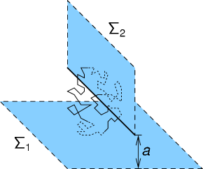
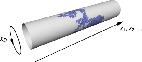
Figure 1: Left panel: sketch of the parallel-plate configuration (taken from [32]). Right panel: sketch of the finite-temperature spacetime; a worldline can wind around the compactified time dimension.

2 Worldline approach to the Casimir effect at finite temperature

Let us briefly summarize the worldline approach to the Casimir effect. More detailed descriptions and derivations from first principles can be found in [11, 16]. We consider the Casimir interaction energy, serving as a potential energy for the force, for two rigid objects with surfaces $\Sigma_{1}$ and $\Sigma_{2}$. For a massless scalar field with Dirichlet boundaries in $D=3+1$, the worldline representation of the Casimir interaction energy is given by

$$E_{\mathrm{Casimir}}=-\frac{1}{2}\frac{1}{(4\pi)^{2}}\int_{0}^{\infty}\frac{d\mathcal{T}}{\mathcal{T}^{3}}\int d^{3}x_{\mathrm{CM}}\,\left\langle\Theta_{\Sigma}[\mathbf{x}(\tau)]\right\rangle.$$ (1)

Here, the worldline functional $\Theta_{\Sigma}[\mathbf{x}(\tau)]=1$ if the path $\mathbf{x}(\tau)$ intersects the surface $\Sigma=\Sigma_{1}\cup\Sigma_{2}$ in both parts $\Sigma_{1}$ and $\Sigma_{2}$, and $\Theta_{\Sigma}[\mathbf{x}(\tau)]=0$ otherwise.

This compact formula has an intuitive interpretation: the worldlines can be viewed as the spacetime trajectories of the quantum fluctuations of the scalar field. Any worldline that intersects the surfaces does not satisfy Dirichlet boundary conditions. All worldlines that intersect both surfaces thus should be removed from the ensemble of allowed fluctuations, thereby contributing to the negative Casimir interaction energy. The auxiliary integration parameter $\mathcal{T}$, the so-called propertime, effectively governs the extent of a worldline in spacetime. Large $\mathcal{T}$ correspond to IR fluctuations with large worldlines, small $\mathcal{T}$ to UV fluctuations.

The expectation value in Eq. (1) has to be taken with respect to the ensemble of worldlines that obeys a Gaußian velocity distribution

$$\langle\dots\rangle={\int_{\mathbf{x}_{\mathrm{CM}}}\mathcal{D}x\,\dots\,e^{-\frac{1}{4}\int_{0}^{\mathcal{T}}d\tau\,\dot{x}^{2}(\tau)}}\Bigg{/}{\int_{\mathbf{x}_{\mathrm{CM}}}\mathcal{D}xe^{-\frac{1}{4}\int_{0}^{\mathcal{T}}d\tau\,\dot{x}^{2}(\tau)}},$$ (2)

where the worldlines have a common center of mass $x_{\mathrm{CM}}$. At zero temperature, the time component of the worldlines cancels out for static objects, hence the straightforward Monte Carlo computation of Eqs. (1) and (2) can be restricted to the spatial part.

Finite temperature can now easily be implemented with the aid of the Matsubara formalism, and also the technical changes of the numerical algorithm are only minor: The Euclidean time, say along the $D$th direction, is compactified to the interval $[0,\beta]$ with periodic boundary conditions for bosonic fluctuations. As a consequence, the worldlines can also wind around the time dimension, see Fig. 1. It is convenient to write a given loop $x(\tau)$ with winding number $n$ as sum of a loop with no winding, $\tilde{x}(\tau)$, and a translation in time running from zero to $n\beta$ with constant speed,

$$x_{\mu}(\tau)=\tilde{x}_{\mu}(\tau)+n\beta\frac{\tau}{\mathcal{T}}\delta_{\mu D}.$$ (3)

The path integral over the different winding number sectors labeled by $n$ factorizes for static configurations, yielding

$$\int_{x(0)=x(\mathcal{T})}\mathcal{D}x\ e^{-\int_{0}^{\mathcal{T}}d\tau\frac{\dot{x}^{2}}{4}}\ \cdots\ =\sum_{n=-\infty}^{\infty}e^{-\frac{n^{2}\beta^{2}}{4\mathcal{T}}}\int_{\tilde{x}(0)=\tilde{x}(\mathcal{T})}\mathcal{D}\tilde{x}\ e^{-\int_{0}^{\mathcal{T}}d\tau\frac{\dot{\tilde{x}}^{2}}{4}}\ \cdots.$$ (4)

The worldline representation of the Casimir interaction energy for the Dirichlet scalar at finite temperature thus reads

$$E_{\mathrm{Casimir}}=-\frac{1}{2}\frac{1}{(4\pi)^{2}}\int_{0}^{\infty}\frac{d\mathcal{T}}{\mathcal{T}^{3}}\biggl{(}\sum_{n=-\infty}^{\infty}e^{-\frac{n^{2}\beta^{2}}{4\mathcal{T}}}\biggr{)}\int d^{3}x_{\mathrm{CM}}\,\left\langle\Theta_{\Sigma}[\mathbf{x}(\tau)]\right\rangle.$$ (5)

Whereas the worldline expectation value remains identical to the one at zero temperature, the winding sum re-weights the propertime integrand: larger temperature emphasizes smaller propertimes and vice versa. This confirms the expectation that thermal corrections at low temperature are dominated by long wavelength fluctuations which in our case correspond to worldlines with a large spatial extent.

It is important to note that $E_{\mathrm{Casimir}}$ is normalized such that $E_{\mathrm{Casimir}}\to 0$ for infinite distances $a\to\infty$. Hence, $E_{\mathrm{Casimir}}$ can differ from the thermodynamic free energy by thermal corrections to the self-energies of the single surfaces. The latter is distance-independent and thus does not contribute to the Casimir force.

2.1 Parallel plates

As a test, let us consider the two parallel plates separated by a distance $a$ along the $z$ axis. Interchanging expectation value and $z_{\mathrm{CM}}$ integration in Eq. (5), we encounter

$$\int_{-\infty}^{\infty}\,dz_{\mathrm{CM}}\,\Theta_{\Sigma}[\mathbf{x}]=(\sqrt{\mathcal{T}}l-a)\,\theta(\sqrt{\mathcal{T}}l-a),$$ (6)

where $l$ denotes the dimensionless extent of the given worldline in $z$ direction measured in units of $\sqrt{\mathcal{T}}$; cf. [16]. Differentiating Eq. (5) by $-\partial/\partial a$ yields the Casimir force

$$F_{\mathrm{Casimir}}=-\frac{1}{2}\frac{A}{(4\pi)^{2}}\,\frac{1}{a^{4}}\left\langle\int_{1/l^{2}}^{\infty}\frac{d\mathcal{T}}{\mathcal{T}^{3}}\biggl{(}\sum_{n=-\infty}^{\infty}e^{-\frac{n^{2}}{4\mathcal{T}}\,\frac{\beta^{2}}{a^{2}}}\biggr{)}\right\rangle,$$ (7)

where $A$ is the (infinite) area of the plates.

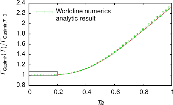
Figure 2: Temperature dependence of the Casimir force between two parallel plates. The ratio of the force at temperature $T$ and at zero temperature is plotted versus the temperature in units of the plate distance $a$. The rectangle at low temperature marks the region magnified in Fig. 3. For the worldline numerical result, we have employed 800 loops each with $1\;000\;000$ points.

Figure 2 shows the numerical result for the Casimir interaction energy (7), corresponding to the distant-dependent part of the free energy, normalized to the zero-temperature result. For comparison, the analytic result,

$$F_{\mathrm{Casimir}}=\frac{\pi^{2}}{2}\frac{\partial}{\partial a}\left[\frac{AT}{a^{2}}\sum_{m=1}^{\infty}\frac{1}{(2\pi m)^{3}}\left(\coth(2\pi maT)+2\pi maT\,\mathrm{csch}^{2}(2\pi maT)\right)\right],$$ (8)

is also shown, see e.g. [33]. Both results agree satisfactorily.

Incidentally, the leading thermal correction can be obtained analytically from the worldline representation (7): for $(aT)^{2}\ll 1$ (and $n\neq 0$), the propertime integrand is dominated by large $\mathcal{T}$, hence the lower bound can safely be set to zero. This results in the well-known leading thermal correction $\Delta F(T)=-(\pi^{2}/90)AT^{4}$, which can also be understood as an excluded volume effect: thermal modes are excluded from the region between the two plates which thus does not contribute to the Stefan-Boltzmann law.

2.2 Perpendicular plates

We now consider the perpendicular-plate configuration introduced above. Again, we can perform the $z_{\mathrm{CM}}$ integration first, yielding for the force

$$F_{\mathrm{Casimir}}=-\frac{L}{2(4\pi)^{2}}\,\frac{1}{a^{3}}\left\langle\int d\xi\int_{1/l(\xi)^{2}}\frac{d{\mathcal{T}}}{\mathcal{T}^{5/2}}\biggl{(}\sum_{n=-\infty}^{\infty}e^{-\frac{n^{2}}{4\mathcal{T}}\,\frac{\beta^{2}}{a^{2}}}\biggr{)}\right\rangle,$$ (9)

where $L$ is the (infinite) length of the system along the edge. Here, $l(\xi)$ denotes the dimensionless extent of the given worldline in $z$ direction as seen by the configuration in units of $\sqrt{\mathcal{T}}$; it depends on the position $\xi$ of the worldline normal to the perpendicular plate which is also measured in units of $\sqrt{\mathcal{T}}$; for details, see [34].

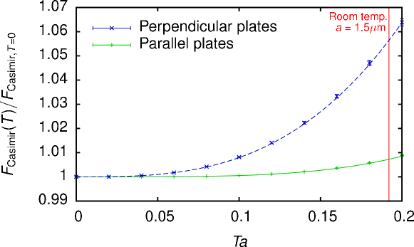
Figure 3: Temperature dependence of the Casimir force for two perpendicular plates compared to the parallel-plates result. The ratio of the force at temperature $T$ and at zero temperature is plotted versus the temperature in units of the plate distance $a$. The plot shows the small-temperature range of Fig. 2. At experimentally relevant large-separation values of $Ta$ (vertical line), the temperature correction for the perpendicular plates is $\simeq 6\%$, which should be compared with $\sim 0.7\%$ for the parallel plates. For the worldline numeric results we have employed 800 loops each with 1 000 000 points. The error bars represent the statistical error.

Figure 3 compares the resulting temperature correction with that of the parallel-plates case in the small temperature range of Fig. 2. In contrast to the weak $(aT)^{4}$ dependence of the parallel-plates result, the Casimir interaction energy for the perpendicular plates shows a strong increase with temperature. For typical experimental values at larger distance $a=1.5\mu$m and room temperature, the temperature correction is about $6\%$. At the same distance and temperature, the temperature effect for the parallel plates is $0.7\%$. The open geometry therefore exhibits a thermal correction which is an order of magnitude larger than the closed parallel-plates case.

The leading thermal correction can again be computed analytically from the worldline representation (9) by extending the lower bound of the $\mathcal{T}$ integral to 0 and using $\langle\int d\xi\rangle\equiv\langle l\rangle=\sqrt{\pi}$. Here, $l$ denotes the extension of the loop perpendicular to the semi-infinite plate [16]. We obtain

$$F_{\mathrm{Casimir}}(T)\simeq F_{\mathrm{Casimir},{T=0}}-\frac{\zeta(3)}{4\pi}\,\frac{L}{a^{3}}\,(aT)^{3},\quad\mathrm{for}\,\,(aT)\ll 1,$$ (10)

which is confirmed by the full numerical result over the whole range of temperatures shown in Fig. 3. We note that the low-temperature scaling of the thermal correction for this open geometry cannot be understood as an excluded-volume effect.

3 Conclusions

We have presented analytical as well as numerical results for the nontrivial interplay between geometry and finite temperature for the Casimir effect in open geometries. For the first time, we have shown that the gapless nature of the fluctuation spectrum leads to a strong enhancement of the thermal correction to the Casimir force. Our numerical data for the perpendicular-plate case with Dirichlet b.c. confirms our analytically derived $(aT)^{3}$ force law at low temperatures. This should be compared to the weaker $(aT)^{4}$ dependence of the parallel-plates case where a gap in the spectrum suppresses the thermal correction. This calls urgently for further first-principles computations for other open geometries such as the sphere-plate case.

It is a pleasure to thank Michael Bordag and his team for the organization of the QFEXT07 workshop and for creating such a stimulating atmosphere. This work was supported by the DFG under Gi 328/1-3 (Emmy-Noether program) and Gi 328/3-2.

References

References

- [1] H.B.G. Casimir, Kon. Ned. Akad. Wetensch. Proc. 51, 793 (1948).
- [2] K. A. Milton, River Edge, USA: World Scientific (2001); M. Bordag, U. Mohideen and V. M. Mostepanenko, Phys. Rept. 353, 1 (2001); S. Y. Buhmann and D. G. Welsch, Prog. Quant. Electron. 31, 51 (2007) [arXiv:quant-ph/0608118].
- [3] B.V. Derjaguin, I.I. Abrikosova, E.M. Lifshitz, Q.Rev. 10, 295 (1956); J. Blocki, J. Randrup, W.J. Swiatecki, C.F. Tsang, Ann. Phys. (N.Y.) 105, 427 (1977).
- [4] G. Feinberg and J. Sucher, Phys. Rev. A 2, 2395 (1970).
- [5] R. Balian and B. Duplantier, Annals Phys. 112, 165 (1978).
- [6] S. K. Lamoreaux, Phys. Rev. Lett. 78, 5 (1997); U. Mohideen and A. Roy, Phys. Rev. Lett. 81, 4549 (1998); H.B. Chan et al., Science 291, 1941 (2001); R.S. Decca et al., Phys. Rev. D 68, 116003 (2003); Phys. Rev. Lett. 94, 240401 (2005).
- [7] M. Schaden and L. Spruch, Phys. Rev. A 58, 935 (1998); Phys. Rev. Lett. 84 459 (2000)
- [8] M. Bordag, D. Robaschik and E. Wieczorek, Annals Phys. 165, 192 (1985).
- [9] T. Emig, A. Hanke and M. Kardar, Phys. Rev. Lett. 87 (2001) 260402.
- [10] M. Brown-Hayes, D.A.R. Dalvit, F.D. Mazzitelli, W.J. Kim and R. Onofrio, Phys. Rev. A 72, 052102 (2005).
- [11] H. Gies, K. Langfeld and L. Moyaerts, JHEP 0306, 018 (2003); arXiv:hep-th/0311168.
- [12] M. G. Schmidt and C. Schubert, Phys. Lett. B 318, 438 (1993) [arXiv:hep-th/9309055]; for a review, see C. Schubert, Phys. Rept. 355, 73 (2001).
- [13] H. Gies and K. Langfeld, Nucl. Phys. B 613, 353 (2001); Int. J. Mod. Phys. A 17, 966 (2002).
- [14] H. Gies and K. Klingmuller, J. Phys. A 39 6415 (2006) [arXiv:hep-th/0511092].
- [15] H. Gies and K. Klingmuller, Phys. Rev. Lett. 96, 220401 (2006) [arXiv:quant-ph/0601094].
- [16] H. Gies and K. Klingmuller, Phys. Rev. D 74, 045002 (2006) [arXiv:quant-ph/0605141].
- [17] T. Emig and R. Buscher, Nucl. Phys. B 696, 468 (2004).
- [18] A. Bulgac, P. Magierski and A. Wirzba, Phys. Rev. D 73, 025007 (2006) [arXiv:hep-th/0511056]; A. Wirzba, A. Bulgac and P. Magierski, J. Phys. A 39 (2006) 6815 [arXiv:quant-ph/0511057].
- [19] T. Emig, R. L. Jaffe, M. Kardar and A. Scardicchio, Phys. Rev. Lett. 96 (2006) 080403.
- [20] M. Bordag, Phys. Rev. D 73, 125018 (2006); Phys. Rev. D 75, 065003 (2007).
- [21] O. Kenneth and I. Klich, Phys. Rev. Lett. 97, 160401 (2006); arXiv:0707.4017.
- [22] T. Emig, N. Graham, R. L. Jaffe and M. Kardar, arXiv:0707.1862; arXiv:0710.3084.
- [23] R. B. Rodrigues, P. A. Maia Neto, A. Lambrecht and S. Reynaud, Phys. Rev. Lett. 96, 100402 (2006) [arXiv:quant-ph/0603120]; Phys. Rev. A 75, 062108 (2007).
- [24] N. Graham, R. L. Jaffe, V. Khemani, M. Quandt, O. Schroeder and H. Weigel, Nucl. Phys. B 677, 379 (2004) [arXiv:hep-th/0309130];
- [25] F. D. Mazzitelli, D. A. R. Dalvit and F. C. Lombardo, New J. Phys. 8, 240 (2006); D. A. R. Dalvit, F. C. Lombardo, F. D. Mazzitelli and R. Onofrio, Phys. Rev. A 74, 020101 (2006).
- [26] M. Boström and Bo E. Sernelius, Phys. Rev. Lett. 84, 4757 (2000).
- [27] V. M. Mostepanenko et al., J. Phys. A 39, 6589 (2006) [arXiv:quant-ph/0512134].
- [28] I. Brevik, S. A. Ellingsen and K. A. Milton, arXiv:quant-ph/0605005.
- [29] A. Scardicchio and R. L. Jaffe, Nucl. Phys. B 743 (2006) 249 [arXiv:quant-ph/0507042].
- [30] M. Bordag, B. Geyer, G. L. Klimchitskaya and V. M. Mostepanenko, Phys. Rev. Lett. 85, 503 (2000).
- [31] A. Scardicchio and R. L. Jaffe, Nucl. Phys. B 704, 552 (2005); Phys. Rev. Lett. 92, 070402 (2004).
- [32] H. Gies and K. Klingmuller, Phys. Rev. Lett. 97, 220405 (2006) [arXiv:quant-ph/0606235].
- [33] J. Feinberg, A. Mann and M. Revzen, Annals Phys. 288 (2001) 103 [arXiv:hep-th/9908149].
- [34] K. Klingmuller, Dissertation, Heidelberg U. (2007).