Twist solitons in complex macromolecules: from DNA to polyethylene

Abstract

DNA torsion dynamics is essential in the transcription process; simple models for it have been proposed by several authors, in particular Yakushevich (Y model). These are strongly related to models of DNA separation dynamics such as the one first proposed by Peyrard and Bishop (and developed by Dauxois, Barbi, Cocco and Monasson among others), but support topological solitons. We recently developed a “composite” version of the Y model, in which the sugar-phosphate group and the base are described by separate degrees of freedom. This at the same time fits experimental data better than the simple Y model, and shows dynamical phenomena, which are of interest beyond DNA dynamics. Of particular relevance are the mechanism for selecting the speed of solitons by tuning the physical parameters of the non linear medium and the hierarchal separation of the relevant degrees of freedom in “master” and “slave”. These mechanisms apply not only do DNA, but also to more general macromolecules, as we show concretely by considering polyethylene.

Introduction

Following the early works of Davydov on solitons in biological systems [13], it has been conjectured since a long time [17] that nonlinear excitations – in particular, kink solitons or breathers – could be present in the DNA double chain and could play a functional role, in particular in the processes of DNA denaturation and transcription.

This general idea meets of course essential difficulties when one tries to translate it into quantitative terms due to the formidable complexity of the DNA molecule [9, 45]. This is organized in two helices; each of them is composed of adjoining nucleotides. A nucleotide consists of a unit of the sugar-phosphate backbone (identical in each nucleotide) and an attached nitrogen base (this can be of four different types; the base at a given site on one chain uniquely determines the base at the same site on the other chain, as they must be one of the Watson-Crick pairs). This makes 30-35 atoms and hence about 100 classical degrees of freedom for each nucleotide; each helix is then made, depending on the species, of $10^{6}-10^{9}$ nucleotides.

In view of the quasi-regular structure of DNA – and despite the fact genetic information is embodied in the non-regular part of the structure – it is quite reasonable to start the modelling by considering a polymer made of identical units (the nucleotides), deferring taking into account the actual base sequence and hence inhomogeneities in the structure to a later moment (and to computer simulations rather than analytical investigation).

Needless to say, DNA like any other molecule actually obeys quantum rather than classical mechanics. The first consequence of this is that nucleotides can be realistically thought as made of rather rigid subunits, and one can just consider the degrees of freedom of these subunits [9, 26, 45]. Under closer scrutiny, it turns out that some of these degrees of freedom are more easily excited and hence dominant, i.e. those related to a radial movement of the bases away from the double helix axis, and those related to rotations of the bases and the sugar ring in a plane nearly orthogonal to the double helix axis; in the standard nomenclature of DNA deformations [9, 45, 26], they correspond respectively to stretch and opening.

These considerations are at the basis of DNA modelling as considered in the Nonlinear Mathematics and Theoretical Physics communities, where one aims at reproducing significant experimental observations on the basis of models with few degrees of freedom per nucleotide. These cannot substitute for more massive quantum chemistry computations, but could identify relevant degrees of freedom, hence help in organizing our understanding of the complex DNA dynamics. It is worth stressing, in this respect, that DNA is not only complex structurally, but also performs a great wealth of biological tasks. It is thus not impossible that one can consider different models of it depending on the biological process one aims at modelling; from this perspective, considering only a few degrees of freedom per nucleotide in a model aiming at a specific mode of DNA dynamics, relevant in a specific process, is quite reasonable despite the underlying overall complexity of the molecule and its spatial organization.

As mentioned above, simple DNA models are primarily focusing on DNA denaturation and transcription; more specifically, they aim at describing the deformation of DNA structure corresponding to the two main degrees of freedom mentioned above, “radial” ones (movement of the bases directly away from the double helix axis), thought to be relevant in DNA denaturation; and “torsional” ones (rotations of the bases and the sugar ring in a plane orthogonal to the double helix axis), thought to be relevant in DNA transcription where local untwisting of the double helix would make possible to RNA Polymerase to access the base sequence without disrupting the double helix [9, 17, 26, 45, 54]; see Figure 1.

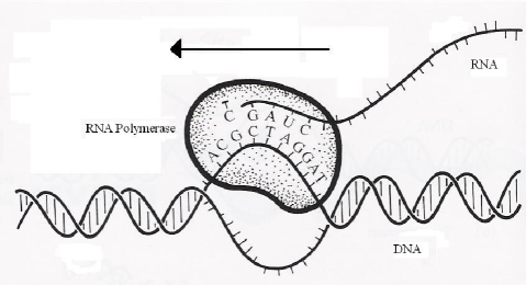
Figure 1: A schematic view of the transcription process. RNA Polymerase reads the bases sequence and produces RNA messenger; the reading requires local unwinding of DNA double helix in a “transcription bubble” region involving about 20 base sites. When active in transcription, RNA Polymerase travels along DNA at a speed of about $0.5-1.0\times 10^{3}$ bases per second, and the transcription bubble moves along the molecule at the same speed. Adapted with modifications from [9].

In this note we will first discuss these models, in particular some concrete models widely studied in the literature, with their success and limitations; and then consider a specific concrete “composite” model we recently proposed for the torsional dynamics and which on the one hand is free of limitations pertaining to other torsional models, and on the other hand shows phenomena which are obviously not specific to it, and could be of interest – theoretical but also applicative – in a much wider nonlinear mechanics context. In order to illustrate this wider applicability, in section 5 we also discuss how these phenomena show up in a different macromolecule, i.e. polyethylene.

We will not discuss DNA structure and its Physics, for which the reader is referred e.g. to [9, 45] and [19, 58] respectively. Experimental studies of single-molecule DNA dynamics are discussed e.g. in [35, 43, 48]; for general discussion of modelling DNA at different scales, see [4].

1 Mechanical models of DNA

A number of mechanical models of the DNA double chain have been proposed over the years, focusing on different aspects of the DNA molecule and on different biological, physical and chemical processes in which DNA is involved. A discussion of such attempts is given in the books by Yakushevich [54] and by Dauxois and Peyrard [42], as well as in the review paper by Peyrard [39].

In recent years, two models have been extensively studied in the Nonlinear Physics literature. These are the “radial” model by Peyrard and Bishop [40] (and the extensions of this formulated by Dauxois [12], Dauxois, Peyrard and Bishop [41], and later on by Barbi, Cocco, Peyrard and Ruffo [1, 2]; see also Cocco and Monasson [11]. More recent advances are discussed in [39] and references therein); and the “torsional” one by Yakushevich [51], which had precursors discussed in [54] and is put in perspective within a hierarchy of DNA models in [52, 53]. We will refer to these as the PB and the Y models respectively.

The interplay between radial and torsional degrees of freedom of bases is considered organically in the Barbi-Cocco-Peyrard (BCP) model [1, 2, 11]; the latter was formulated as an extension of the Peyrard-Bishop-Dauxois model [40, 41], i.e. in the context of “radial” dynamics.

1.1 The PB model

In PB-like models, the bases can only move radially away from the double helix axis. The potential energy corresponds to stacking interactions between successive bases on each chain, and pairing interactions between bases at corresponding sites on opposite chains [9, 26, 42, 45].

We denote by $r_{n}^{(\pm)}\in\mathcal{R}_{+}$ the position of the base at site $n$ on the helix ${(\pm)}$. It is convenient, for our present purposes, to limit discussion of this and other models to symmetric configurations, i.e. configurations with $r_{n}^{(+)}(t)=r_{n}^{(-)}(t)=r_{n}(t)$ at all times. In this case, the Lagrangian describing the PB model is (with $m$ the mass of bases)

$${\mathcal{L}}_{{\rm PB}}\ =\ \sum_{n}m(\dot{r}_{n})^{2}\ -\ K_{s}\,\left(r_{n+1}-r_{n}\right)^{2}\ -\ V_{p}(r_{n})\ .$$ (1)

In the PB model, $V_{p}$ is a Morse potential with a minimum at the equilibrium position, corresponding to $r_{n}=\rho\simeq 2\AA$:

$$V_{p}(r)\ =\ D\,\left(\exp\left[-\alpha(r-\rho)\right]-1\right)^{2}\ .$$ (2)

The Euler-Lagrange (EL) equations for ${\mathcal{L}}_{{\rm PB}}$ are of course

$$m\ddot{r}_{n}\ =\ \,K_{s}\,(r_{n+1}-2r_{n}+r_{n-1})\ -\ \frac{1}{2}{V_{p}}^{\prime}(r_{n})\ .$$ (3)

We will pass to consider the continuum approximation for these, i.e. substitute the infinite array of scalar variables $\{r_{n}(t)\}$ with the interpolating field $R(x,t)$, such that $R(n\delta,t)\approx r_{n}(t)$; here $\delta\simeq 3.4\AA$ is the distance between successive base pairs positions along the double helix axis. Using now a second order approximation,

$$R(x\pm\delta,t)\approx R(x,t)\pm\delta R_{x}(x,t)+(\delta^{2}/2)R_{xx}(x,t)\ ,$$ (4)

and writing for short $\kappa=K_{s}\delta^{2}$, the (3) yield the nonlinear wave equation

$$mR_{tt}\ =\ \kappa\,R_{xx}\ -\ (1/2)[dV(R)/dR]\ .$$ (5)

It can be shown that this supports breathers; their size and oscillation frequency (choosing parameters so that $V_{p}$ describes as far as possible a Hydrogen-bond interaction) are compatible with those observed in real DNA. The discrete model can be put in a thermal bath and numerically simulated, and again one observes a behavior compatible with the one observed in DNA denaturation [39, 42]. More refined versions of this model [41] consider modified expressions for the stacking energy, improving – also qualitatively – the correspondence with actual DNA behavior; we refer again to [39, 42] for details.

1.2 The Y model

In the simple models for DNA torsional dynamics, one studies a system of nonlinear equations which in the continuum limit reduce to a pair of sine-Gordon (SG) type equations; the relevant nonlinear excitations are kink solitons – which are solitons in both dynamical and topological sense – which describe the unwinding of the double helix in a “bubble”.

The main biological interest of these model lies in the identification of this unwound bubble with the transcription region (this is indeed an “open bubble” of about 20 bases, to which RNA Polymerase (RNAP) binds; the RNAP travels along the DNA double chain, and so does the unwound region). The idea of Englander et al. [17] was that the open bubble could correspond to nonlinear excitations and thus be present due to the nonlinear dynamics of the DNA double helix itself; the RNAP would then use them to travel along DNA. In this way a number of questions – in particular, concerning energy flows – would receive a simple explanation. Note that their model, and subsequent ones continuing their research, are not concerned with the DNA-RNAP complex, but the dynamics of the DNA double helix alone.

To be specific, let us consider the model proposed by Yakushevich (see e.g. [54] for similar models proposed earlier on by other authors, starting with [18, 50, 56]); now the degrees of freedom for the rotation of the base at site $n$ on the chain $(\pm)$ will be denoted as $\varphi_{n}^{(\pm)}$, and again we restrict to the symmetric case, i.e. enforce $\varphi_{n}^{(+)}(t)=\varphi_{n}^{(-)}(t)=\varphi_{n}(t)$ at all times (this makes that in the continuum approximation we will get a single equation of SG type rather than two coupled ones). The Lagrangian describing the Y model is (here $m$ is a moment of inertia)

$${\mathcal{L}}_{{\rm Y}}\ =\ \sum_{n}m(\dot{\varphi}_{n})^{2}\ -\ K_{s}\,\left(\varphi_{n+1}-\varphi_{n}\right)^{2}\ -\ \widehat{V}_{p}(\varphi_{n})\ ;$$ (6)

the choice by Yakushevich for the intrapair potential was that of a simple harmonic potential [51], resulting in (we stress here $r$ is a geometrical constant, not a dynamical variable!)

$$\widehat{V}_{p}(\varphi)\ =\ -4K_{p}r^{2}\,\cos(\varphi)\ .$$ (7)

The EL equations for ${\mathcal{L}}_{{\rm Y}}$ are a set of sine-Gordon coupled equation,

$$m\ddot{\varphi}_{n}\ =\ K_{s}\,(\varphi_{n+1}-2\varphi_{n}+\varphi_{n-1})\ -\ (1/2)\,{\widehat{V}_{p}}^{\prime}(\varphi_{n})\ .$$ (8)

Passing to continuum approximation with interpolating field $\Phi(x,t)$ (where $\Phi n\delta,t)\approx\varphi_{n}(t)$, like above) and second order approximation

$$\Phi(x\pm\delta,t)\approx\Phi(x,t)\pm\delta\Phi_{x}(x,t)+(\delta^{2}/2)\Phi_{xx}(x,t)\ ,$$ (9)

the (8) reduce to a sine-Gordon equation

$$m\Phi_{tt}\ =\ \kappa\Phi_{xx}\ -\ \lambda\,\sin(\Phi)\ ;$$ (10)

here of course we have made use of the explicit form of $\widehat{V}_{p}$, set $\lambda=2K_{p}r^{2}$, and defined $\kappa$ as above.

As well known, the sine-Gordon equation supports topological soliton solutions [16]; these solutions are also solitons in the dynamical sense [10]. The basic soliton solution with speed $v$ is

$$\Phi(x,t)\ =\ 4\,{\rm arctan}\left[\exp(\beta(x-vt))\right]\ ,$$ (11)

where we have written

$$\beta=\sqrt{\frac{2K_{p}r^{2}}{-\mu}}\ ,\ \ \mu=m^{2}v^{2}-K_{s}\delta^{2}\ .$$ (12)

Note that $v$ is a free parameter, subject to the condition $|v|<v_{*}=\sqrt{K_{s}}(\delta/m)$. A selection of the speed based on energy is also not present, as the soliton energy has a very weak dependence on its speed except for $v\simeq\pm v_{*}$, see [21].

It has been shown that the Y model gives a correct prediction of quantities related to small amplitude dynamics, such as the frequency of small torsional oscillations; and also of quantities related to fully nonlinear dynamics, such as the size of solitonic excitations describing transcription bubbles [26, 54].

On the other hand, the Y model is not capable of providing a satisfactory prediction for other quantities: in particular, if we try to fit the observed speed of transversal waves along the chain [54], this is possible only upon assuming unphysical values for the coupling constants [55]. That is, with a physical value of the parameters – in particular, for $K_{s}\approx 120{\rm KJ/mol}$ – the Y model predicts a speed $v\approx 320{\rm m/s}$, while in order to get a speed of the order of 2 Km/s as observed in experiments and [32, 55] one has to take $K_{s}\approx 6000$.

Finally, we stress once again that the Y model, like the PB one and unlike the BCP one, assumes that there is a single (angular in this case) degree of freedom for each nucleotide.

1.3 The BCP model

In the BCP model [1, 2, 39, 42], the state of each base is described by both a radial $r_{n}^{(\pm)}$ and an angular $\varphi_{n}^{(\pm)}$ variable. Restricting again to symmetric configurations, and using variables $\{r_{n},\varphi_{n}\}$, the BCP Lagrangian is

$$\begin{array}[]{rl}{\mathcal{L}}_{{\rm BCP}}\ =&\sum_{n}m(\dot{r}_{n}^{2}+r_{n}^{2}\dot{\varphi}_{n}^{2})\ -\ \sum_{n}V_{p}(r_{n})\ +\\ &\ -\ \sum_{n}K_{s}\left(L-\sqrt{\delta^{2}+r_{n+1}^{2}+r_{n}^{2}-2r_{n+1}r_{n}\cos(\varphi_{n+1}-\varphi_{n})}\right)^{2}\ +\\ &\ -\ \sum_{n}G_{0}(\varphi_{n+1}-2\varphi_{n}+\varphi_{n-1})^{2}\ ,\end{array}$$ (13)

with $V_{p}$ the same Morse potential as above (in the non symmetric case, pairing would depend on $\phi$ variables as well) and $L$ the equilibrium distance between bases in three-dimensional space. As for the last term in (13), this is a curvature term whose role is to avoid “zig-zag” configurations, possible for $G_{0}=0$; it should thus be omitted in the continuum approximation.

In this case, proceeding as above (or more simply using the continuum version of the Lagrangian) one obtains [28, 39, 40] in the continuum approximation the EL equations

$$\begin{array}[]{rl}mR_{tt}\ =&mR\Phi_{t}^{2}-\gamma(RP_{x}^{2}-R_{xx})-(1/2)V^{\prime}(R)\ ,\\ mR^{2}\Phi_{tt}\ =&-2mRR_{t}\Phi_{t}+\gamma(R^{2}\Phi_{xx}+2RR_{x}\Phi_{x})\ .\end{array}$$ (14)

It has been shown that for $L>\delta$ this supports nontrivial topological soliton solutions; the determination of these reduces to the study of a single equation thanks to an exact conservation law (the model is invariant by global rotations), but solitons are only determined numerically [28].

The BCP model is quite successful in describing breather excitations of the DNA double chain, and its predictions (or those of the cognate CM model) fit well experimental observations [39, 40] related to the DNA denaturation process.

2 Composite model of DNA torsional dynamics

A closer look at nucleotides structure and conformation [9, 45] shows that torsional motions can take place both as a rotation of the nitrogen base with respect to the sugar ring and as a rotation of the sugar-phosphate group; it should be stressed that the former one is subject to steric hindrances, i.e. is limited by interactions with other parts of the DNA molecule.

Thus, one should consider “composite” torsional models, in which we describe the state of each nucleotide by two independent angular degrees of freedom, one related to the sugar-phosphate group and one to the nitrogen base; see Figure 2 for details. Note that in this scheme one is not considering “radial” (stretch) motions.

2.1 The model

Such a model, described graphically in Figure 2, was recently put forward and studied by three of us [5] (see also [6] for a discussion of it focusing on its mathematical features); it shows some phenomena – to be discussed in later sections – which are not specific to it but apply to a more general class of models and could be of interest in fields quite far from DNA dynamics [7, 8].

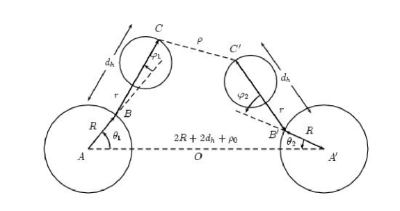
Figure 2: A base pair in the composite Y model (reproduced from [5]). The origin of the coordinate system is in O; the angles $\theta_{1}$ and $\theta_{2}$ correspond to torsion of sugar-phosphate backbone with respect to the equilibrium B-DNA conformation; the angles $\varphi_{1}$ and $\varphi_{2}$ between A’B’ and B’C’ correspond to rotation of bases around the $C-N$ bond linking them to the nucleotide. All angles are in counterclockwise direction.

Our model can be considered as an extension of the Y model. It turns out that the simple Y model captures to a large extent the essential features of the nonlinear dynamics of the composite model. On the other hand, the more realistic geometry of the composite model yields a relevant improvement of the descriptive power of the model at both the conceptual and the phenomenological level; in particular, the composite Y model allows for a more realistic choice of the physical parameters.

The different degrees of freedom we use will play a fundamentally different role in the description of DNA nonlinear dynamics. The backbone degrees of freedom (recall the rotations they describe are not limited) are “topological” and play to some extent a more relevant role, in that the solitons are mainly associated to them; while those associated to the base (recall the associated rotations are subject to steric hindrances) are “non topological” and represent small oscillations. These different roles are specially clear when we consider the limit in which our model reduces to the standard Y model, in which only the topological degrees of freedom are present.

It should be stressed that this feature is specially interesting in connection with the possibility (discussed elsewhere [14]) to consider more realistic models, in which differences among bases are properly considered, as perturbations of our idealized uniform model. As the essential features of the fully nonlinear dynamics are related only to backbone degrees of freedom, such a perturbation should be expected to show the same kind of nonlinear dynamics as our uniform model.

The Lagrangian defining the composite Y model will be written as

$${\mathcal{L}}_{{\rm cY}}\ =\ T\ -\ \left(U_{t}\ +\ U_{s}\ +\ U_{p}\right)\ -\ U_{c}$$ (15)

with $T$ the kinetic energy, $U_{t}$ is the backbone torsional potential, $U_{s}$ the stacking potential, and $U_{p}$ the pairing potential.

Moreover $U_{c}$ is a constraining potential which represents the steric hindrances to the base rotations (not accompanied by sugar-phosphate rotations); its explicit expression is to a large extent arbitrary, provided $\varphi_{n}$ are de facto bound to a small range around zero.

Explicit expressions for the potentials are rather involved [5] and will be given below in (16), considering again symmetric configurations only for the sake of simplicity (see [5, 6] for the general case). Note in there $r$ and $R$ are geometrical parameters (and $m$, $I$ represent masses and inertia moments), while the dynamical variables are $\{\varphi_{n}(t),\vartheta_{n}(t)\}$, $n\in{\bf Z}$.

Before writing these explicit expressions, we state that $U_{t}$ and $U_{s}$ correspond to the torsional energy of the backbone and the base stacking energy respectively, and have simple harmonic expressions in terms of the three-dimensional coordinates of involved nucleotide elements (albeit a rather involved expression in terms of torsion angles); as for the pairing interaction $U_{p}$, this corresponds again to a harmonic potential in three-dimensional distance between bases in a pair. This latter choice, albeit not natural physically (a Morse potential as in the PB or BCP models would perhaps be more appropriate; see [24] for a discussion of different intrapair potentials within the Y model) was made in order to ease comparison with results obtained for the simple Y model, i.e. in order to focus attention on the improvements which have to be ascribed to the geometry of the model. Here are the explicit expressions for $T$ and the $U_{i}$:

$$\begin{array}[]{rl}T\ =&\frac{1}{2}\ \sum_{n}\ \left[m\,r^{2}\,\left(\dot{\varphi}_{n}\right)^{2}\ +\ 2\,m\,r\,(r+R\cos(\varphi_{n}))\,\dot{\vartheta}_{n}\,\dot{\varphi}_{n}\ +\right.\\ &\left.+\ \left(I+m(R^{2}+r^{2})+2mRr\cos(\varphi_{n})\right)\left(\dot{\vartheta}_{n}\right)^{2}\right]\ ;\\ U_{t}\ =&\ K_{t}\ \sum_{n}\,\left[1\,-\,\cos\left(\vartheta_{n+1}-\vartheta_{n}\right)\right]\ ;\\ U_{s}\ =&\ K_{s}\ \sum_{n}\ 2\,\left[R^{2}+r^{2}\ +\right.\\ &\left.-\ R^{2}\cos(\vartheta_{n+1}-\vartheta_{n})\,-\,r^{2}\cos[(\vartheta_{n+1}-\vartheta_{n})+(\varphi_{n+1}-\varphi_{n})]\ +\right.\\ &\left.-\ Rr\left(\cos[(\vartheta_{n+1}-\vartheta_{n})+\varphi_{n+1}]+\cos[(\vartheta_{n+1}-\vartheta_{n})-\varphi_{n}]\right)\ +\right.\\ &\left.+\ Rr\left(\cos(\varphi_{n+1})+\cos(\varphi_{n})\right)\right]\ ;\\ U_{p}\ =&\ (1/2)\,K_{p}\ \sum_{n}\,(\sigma_{n}-\rho)^{2}\ ,\ {\rm with}\\ \sigma_{n}^{2}\ =&\ 4\left[a^{2}+R^{2}+d_{h}^{2}+2\left(Rd_{h}\cos\varphi_{n}-aR\cos\vartheta_{n}-ad_{h}\cos(\varphi_{n}+\vartheta_{n})\right)\right]\ .\end{array}$$ (16)

Here $m$ is the base mass, $I$ the momentum of inertia of the disk modelling the backbone units and and $K_{t},K_{s},K_{p}$ are, respectively the torsional, stacking and pairing coupling constants; $\sigma_{n}$ represents the distance between bases in a pair (between end points of double pendulums), so that $U_{p}$ is a harmonic potential in the physical distance, albeit expressed by a non-harmonic function when dealing with angular variables.

We work in the so-called contact approximation in which the equilibrium distance between the two basis, $\rho_{0}$ vanishes (see Figure (2). In this approximation the parameter $a$ appearing above is given by $a=R+d_{h}$. Proceeding as in the PB, Y and BCP cases above, we obtain field equations for the interpolating fields $\Phi(x,t)$ and $\Theta(x,t)$; these are rather lengthy and reported explicitly in Appendix B of [5]. As we are mainly interested in soliton equations, we will introduce the travelling wave ansatz

$$\Phi(x,t)=\Phi(x-vt)=\phi(z)\ ,\ \ \Theta(x,t)=\Theta(x-vt)=\theta(z)\ .$$ (17)

The equations for travelling wave (TW) solutions are

$$\begin{array}[]{l}\mu r^{2}\,\phi^{\prime\prime}\ +\ \mu r(r+R\cos\phi)\,\theta^{\prime\prime}\ =\\ \ \ =\ -2aK_{p}(a-R)\,\sin\left(\phi+\theta\right)+K_{s}\delta^{2}Rr\,\sin\left(\phi\right)\,(\theta^{\prime})^{2}\ +\\ \ \ \ -R\,\sin(\phi)\,(-2K_{p}(a-R)+mrv^{2}(\theta^{\prime})^{2})-\frac{dU_{c}}{d\phi}\ ;\\ \mu r(r+R\cos\phi)\,\phi^{\prime\prime}\ +\ [J+\mu(R^{2}+r^{2}+2Rr\cos\phi)\,\theta^{\prime\prime}\ =\\ \ \ =\ -2aK_{p}\left(R\sin\theta+(a-R)\sin(\phi+\theta)\right)+\mu Rr\,\sin(\phi)[(\phi^{\prime})^{2}+2\phi^{\prime}\theta^{\prime}]\ .\end{array}$$ (18)

Here we have simplified the notation by introducing the constants

$$\mu\ =\ (mv^{2}-K_{s}\delta^{2})\ ,\ \ J\ =(Iv^{2}-K_{t}\delta^{2})\ .$$ (19)

It should be stressed that the ODEs (18) are obtained as a reduction of the nonlinear wave PDEs for $\Phi$ and $\Theta$; the latter should be supplemented by boundary conditions. Requiring that the solutions go to an equilibrium for $x\to\pm\infty$ (and thus have finite energy), these are $\Phi(\pm\infty,t)=\Phi_{x}(\pm\infty,t)=\Phi_{t}(\pm\infty,t)=0$, $\Theta(\pm\infty,t)=2n_{\pm}\pi$, $\Theta_{x}(\pm\infty,t)=\Theta_{t}(\pm\infty,t)=0$. These entail side conditions for $\phi(z)$ and $\theta(z)$, i.e.

$$\phi(\pm\infty)=0\ ,\ \theta(\pm\infty)=2n_{\pm}\pi\ ;\ \ \phi^{\prime}(\pm\infty)=0\ ,\ \theta^{\prime}(\pm\infty)=0\ .$$ (20)

We also note that the constraining potential $U_{c}$ makes that the fields $(\Theta,\Phi)$, which in principles take values in $S^{1}\times S^{1}$, are actually taking values in $S^{1}\times I_{0}$ (where $I_{0}=(-\lambda,\lambda)$ is a real interval centered in zero, with $\lambda\ll\pi$); thus $\Theta$ is a topological field, while $\Phi$ is a non-topological one (that is why the boundary conditions for $\Phi$ do not allow nontrivial multiples of $2\pi$).

2.2 Physical values of the parameters

One of the nice and striking features of our composite model is that it supports solitonic solutions within a fully realistic range of all the physical parameters characterizing the DNA; this should be compared with the situation for simple torsional models mentioned above, where unphysical coupling constants are needed to fit some experimental data.

Let us therefore briefly discuss how the values of the parameters appearing in Eq. (16) are fixed.

There are basically two types of parameters: kinematical ( the geometrical parameters $R,r,d_{h},a$, the mass $m$ and the momentum of inertia $I$), and dynamical (the elastic coupling constants $K_{t},K_{s},K_{p}$ )

The kinematical parameters can be evaluated by considering the chemical structure and the geometry of the DNA molecule. The order of magnitude of the mean value of the bases mass is $m\sim 130$ (atomic units). For the momentum of inertia of the disk we have $I\sim 5\times 10^{-44}\,{\rm Kg\,m}^{2}$, whereas the values of the geometrical parameters are given in Table 1.

$R$	$r$	$d_{h}$	$a$
3.1 Å	2.7 Å	4.4 Å	7.5 Å

Table 1: The geometrical parameters in the composite DNA model.

The determination of the numerical values of the coupling constants characterizing our model is more involved. Their order of magnitude can be estimated by considering the typical energy of hydrogen bonds ($K_{p}$) and the experimental results for the torsional rigidity of the DNA chain ($K_{s}$ and $K_{t}$) [5]. The results are given in Table 2.

$K_{t}$	$K_{s}$	$K_{p}$
130 KJ/mol	16.6 N/m	3.5 N/m

Table 2: The dynamical parameters in the composite DNA model.

These values allow in particular to estimate the speed of torsion waves associated to base torsion; this will be the speed of transverse elastic waves along the double chain.

With the above values, the speed of elastic waves is estimated to be $v_{s}=\delta\sqrt{K_{s}/m}\approx 3{\rm Km/s}$; this is of the right order of magnitude, and well compatible with experimental data [32, 59].

Let us stress that the geometry of our composite model makes that using natural parameters one obtains predictions that nicely fits with the estimates of the structural properties and binding energies of the DNA: the induced optical frequencies and phonon speeds are of the same order of magnitude of those experimentally observed. This does not happen in simpler models, as stressed above when discussing the simple Y model.

2.3 Nonlinear dynamics and soliton solutions

Equations (18) are a system of two coupled, non linear ODEs. In general it cannot be solved analytically in closed form. One has to resort to numerical calculations in order to show that the system admits solutions satisfying the boundary conditions (20) [5] (see also Ref. ([14]).

We note that the relevance of the dynamical system (18) goes well beyond DNA torsional dynamics: the same kind of equations appear in more general cases.

In fact, we can as well consider (18) as describing the continuum limit of the torsional dynamics of a single molecular chain made of a disk and a pendulum. In this case, the pairing interaction for the DNA double chain is replaced by an external potential:

$$V=-4r^{2}K_{p}\left(\cos\theta+\cos(\varphi+\theta)-\frac{1}{2}\cos\varphi-3/2\right)\ ,$$ (21)

whereas the stacking and torsional interaction generate the $x$-derivative terms.

To further simplify our model – and the resulting explicit formulas – and concentrate on essential features of interest also beyond DNA dynamics, we also set $R=r$ in (18). The resulting equations take the much simpler form

$$\begin{array}[]{l}\mu\,\phi^{\prime\prime}\ +\ \mu(1+\cos\phi)\,\theta^{\prime\prime}\ =\\ \ \ \ \ =\ -4K_{p}\,\sin\left(\phi+\theta\right)-\mu\,\sin\left(\phi\right)\,(\theta^{\prime})^{2}\ +\ 2K_{p}\,\sin(\phi)-\frac{\partial U_{c}}{\partial\phi}\ ;\\ \mu(1+\cos\phi)\,\phi^{\prime\prime}\ +\ [(J/r^{2})+2\mu(1+\cos\phi)]\,\theta^{\prime\prime}\ =\\ \ \ \ \ =\ -4K_{p}\left(\sin\theta+\sin(\phi+\theta)\right)+\mu\,\sin(\phi)[(\phi^{\prime})^{2}+2\phi^{\prime}\theta^{\prime}]\ ,\end{array}$$ (22)

The previous form of the equations of motion will be taken as starting point to discuss two general features of the dynamical system. As we will see in the next two sections these features (the existence of a mechanism to select the speed of solitonic solutions and the slaving of the field $\phi$) represent quite general consequences of nonlinear dynamics. We expect they will have a quite broad field of application in the context of non-linear Physics and Mechanics.

Although in the general case one can find a solitonic solution of the system (22) only numerically, there is a particular case which admits analytical solutions. This is obtained by freezing the angle $\phi$, i.e by setting $\phi=0$; note that if we force $\phi(z)=0$, we are actually considering a chain of simple pendulums, i.e. a sine-Gordon equation.

This constraint can be accommodated in our setting in a dynamical way, by acting on the confining potential $U_{c}$: this should be made stronger and stronger and the maximum angle $\phi_{0}$ will become smaller and smaller.

Setting $\phi=0$ and using $(\partial U_{c}/\partial\phi)(0)=0$, the system (22) is equivalent to the equation

$$\mu\theta^{\prime\prime}=-2K_{p}\sin\theta\ ;$$ (23)

the compatibility condition between the two equations of the system (22) is now given by

$$J=0.$$ (24)

Equation (23) has to be integrated with the boundary conditions (20). When $\mu<0$ and $n=1$, we have the kink

$$\theta_{0}=4\arctan[e^{\beta z}],\quad\quad\phi=0\ ,$$ (25)

where we have written, as in (12), $\beta=\sqrt{\frac{2K_{p}}{-\mu}}$. The solution (25) is of course the same as (11), i.e. the solution found in the context of the simple Y model.

As for general solutions, we note these will still be indexed by the topological index $n$ (which refers to the $\theta$ behavior); the full equations (22) cannot be solved analytically in the general case (see below for a perturbative approach), but they can be studied and solved numerically; the solution for $n=1$ is displayed in Figure 3.

Figure 3: The $n=1$ soliton for the composite model of Figure 2. We plot in thick curves the fields $\theta$ (on the left) and $\phi$ (on the right) as a function of $x$ for the static ($v=0$) solution with physical values for the model parameters (reproduced from [6]). The solution is very similar to the corresponding one obtained for the Y model for what concerns the $\theta$ field.

2.4 Discussion

It is quite clear that a weak point of this model is represented by the choice of the exceedingly simple potential $U_{p}$; and also by the the simplifying assumption $\rho=0$ (see (16) and comments thereafter).

As mentioned above, this choice was justified by the will to ease comparison with results obtained with the simple Y model, i.e. to be able to focus on new features depending only on the more articulated geometry of the model.

Needless to say, one should then consider the same model with more realistic pairing potentials – e.g. with the Morse potential used in the PB and BCP models (this is being done [14], and yields quite interesting preliminary results).

It should be mentioned, in this respect, that investigations conducted within the framework of the simple Y model have shown that while dispersion relations are of course strongly affected by the contact approximation and by the choice of the pairing potential, these have very little effect on the soliton equations (provided parameters in the pairing potential are set obeying to the same physical argument and considerations); this is shown in Figure 4.

Figure 4: Comparison of the standard Yakushevich $n=1$ soliton (11) (dotted curves) with the $n=1$ solitons (solid curves) obtained numerically by relaxing the $\ell_{0}=0$ contact approximation (left, from [23]) and with a Morse rather than harmonic intrapair potential (right, from [24]). This clearly shows solitons solutions are very little affected by the simplifying choices used in the Y model.

3 Soliton’s speed selection

A general feature of sine-Gordon solitons (and more in general of relativistic solitons) is that the soliton speed $|v|$ is a free parameter, which can be fixed by choosing initial conditions and is bounded from above by a limiting value $c_{0}$. This is a consequence of the Lorentz symmetry of the equation that fixes a limiting upper bound for the speed, whereas $v$ can be changed by applying a boost.

Very often it happens that non-linear systems (e.g the DNA chain, but also reaction-diffusion equations [38], tsunami equations [34], etc.) that allow for solitary, non dispersive excitations, somehow select the order of magnitude for the speed of propagation of this excitation, in the sense that when solitons are experimentally observed, they turn out to have a speed of a well defined order of magnitude.

Thus, in practical situations, whenever the experiments give a well-defined value for the propagation speed of the soliton, the speed degeneracy represents a loss of predictive power of the model. It is quite remarkable that our model has a built-in mechanism for selecting the soliton speed; it is essential for this mechanism that we have (at least) a two-components system.

3.1 Speed selection in the composite DNA model

One can easily realize that the compatibility condition (24) fixes the speed of propagation of the soliton (25) to the speed $c_{t}$ of the transverse sound waves supported by the elastic torsional forces acting on the disk

$$v=c_{t}=\sqrt{\omega_{t}/I},$$ (26)

where $\omega_{t}=K_{t}\delta^{2}$.

Moreover, as the soliton exist only for $\mu<0$, the soliton speed is bounded from above by the speed $c_{s}$ of transverse sound waves supported by the elastic stacking forces acting on the pendulum, i.e.

$$v\leq c_{s}=\sqrt{\omega_{s}/m},$$ (27)

where $\omega_{s}=K_{s}\delta^{2}$. In view of Eq. (26), this implies a constraint on the stacking, torsional coupling constants and kinematical parameters of the system:

$$\frac{K_{t}}{I}<\frac{K_{s}}{m}.$$ (28)

This selection mechanism for the soliton speed gives a nice and simple way to produce solitons with a given speed in double pendulums molecular chains. To select the soliton speed one just needs to tune the torsional and stacking coupling constants and the kinematical parameters of the chain such that Eqs. (26) and (28) are satisfied. Acting on the confining potential $U_{c}$, making it stronger and stronger, one obtains the single pendulum limit of the double pendulums chain. The angle is frozen to $\phi=0$ and a SG soliton with a speed equal to that of the transverse sound waves supported by the torsional forces acting on the disk is selected.

Notice that the mechanism described here can be obviously used to devise and realize non-linear media where solitons propagate at a given fixed speed.

3.2 Speed selection in general models

The mechanism for selecting the soliton speed described above for the molecular chain model (22) is rather generic. It is related to the existence of a conditionally conserved quantity $J$ and it is rather independent from the specific form of the interactions characterizing the model. The proposed mechanism will work whenever we have a nonlinear mechanical system satisfying some general conditions:

1. The system must have at least two degrees of freedom ($X,Y$) at each site, which in the continuum approximation will give two interpolating fields ${\hat{X}}(x,t),\,{\hat{Y}}(x,t)$ and are characterized by masses (or moments of inertia) $m,M$ with $m\neq M$;

2. There should be at least two types of interactions: $(a)$ An elastic force (coupling constant $K_{t}$) originated by the interaction between neighboring sites on the chain; $(b)$ A non linear force (coupling constant $K_{p}$) acting on the single site;

3. There should be a confining potential $U_{c}$ that limits the range of variation of one degree of freedom (e.g $Y$) and allows to freeze $Y$. That is, by making $U_{c}$ steeper and steeper we implement the dynamical reduction from two degrees of freedom to one single degree of freedom $X$;

4. Freezing the degree of freedom $Y$ we have both a conservation law for the momenta conjugate to $X$ and solitonic solutions for ${\hat{X}}$.

4 Perturbative expansion and slaving

A drawback of the general composite Y models (16) is that the equations describing its dynamics are far too complex to be exactly solved.

On the other hand, the doubling of degrees of freedom introduces a natural separation between topological and non-topological degrees of freedom. This separation, together with the fact that the composite model allows for the exact Y soliton (25) when the non-topological field $\phi$ is frozen, opens the way to a perturbative treatment of our model.

The simplest way to deal with our non linear system at the perturbative level, is to consider it as embedded in a family of double pendulums chains, which has a single pendulum chain as a special case.

We will first consider a chain of simple pendulums (of length $R$ and mass $M$); we will then look for solutions of the double pendulums model by perturbing the system near the single pendulum Y solutions (25).

As the simple pendulum limit of our double pendulums chain involves a reduction of the number of degree of freedom, we will have to deal with a singular perturbative expansion.

A way to obtain the simple pendulums chain (and the sine-Gordon equation in the continuum limit) from our model is to let the length of second pendulums go to zero. In this case our set of parameters becomes redundant, as the positions of the masses of the pendulums coincide in space, so that only the total mass is relevant. A similar argument can be used to show that only the total coupling strength $\widehat{K}=K_{s}+K_{t}$ is relevant.

If the double pendulums chain is seen as a (singular) perturbation of the simple pendulums, one is naturally led to look for travelling wave solutions as perturbations of the standard sine-Gordon solitons.

This means we look for solutions to the equations (18) in the form of a series expansion in a small parameter $\varepsilon$. We will correspondingly also expand in the same parameter the parameters appearing in the model and in the solution: the geometrical parameters, the masses appearing in our model, the two coupling constants $K_{t}$ and $K_{s}$ and also allow for modification of the speed by expanding it as well [30, 57].

Therefore, the series expansion we adopt are as follows:

$$\begin{array}[]{lll}\vartheta&=\ \vartheta_{0}+\varepsilon(\delta\theta)&=\ \vartheta_{0}+\varepsilon\vartheta_{1}+\varepsilon^{2}\vartheta_{2}+....\ ,\\ \phi&=\ \varepsilon(\delta\phi)&=\ \varepsilon\phi_{1}+\varepsilon^{2}\phi_{2}+....\ ;\\ r&=\ \varepsilon(\delta r)&=\ \varepsilon r_{1}+\varepsilon^{2}r_{2}+...\ ,\\ R&=\ A-\varepsilon(\delta r)&=\ A-\varepsilon r_{1}-\varepsilon^{2}r_{2}-...\ ;\\ m&=\ \varepsilon(\delta m)&=\ \varepsilon m_{1}+\varepsilon^{2}m_{2}+...\ ,\\ M&=\ M_{tot}-\varepsilon(\delta m)&=\ M_{tot}-m_{0}-\varepsilon m_{1}-\varepsilon^{2}m_{2}-...\ ;\\ v&=\ v_{0}+\varepsilon(\delta v)&=\ v_{0}+\varepsilon v_{1}+\varepsilon^{2}v_{2}+...\ ;\\ K_{t}&=\ \varepsilon(\delta\widehat{K})&=\ \varepsilon k_{1}+\varepsilon^{2}k_{2}+...\ ,\\ K_{s}&=\ \widehat{K}-\varepsilon(\delta\widehat{K})&=\ \widehat{K}\,-\varepsilon k_{1}-\varepsilon^{2}k_{2}-...\ .\end{array}$$ (29)

where $\vartheta_{0}$ and $\phi_{0}$ are the limiting simple pendulum solutions given by (25).

Inserting the series expansions (29) in the equations for TW solutions (18) we will obtain perturbative solutions of our non linear dynamical system at the various order of the perturbative expansion in the parameter $\varepsilon$.

We will skip here the computational details, which can be found in Ref. [6, 8]; the results one obtains in this way are summarized as follows.

• At zero order of the perturbation theory the single pendulum solitonic solution (25) is reproduced.

• First and higher order corrections to $\vartheta_{0}$ and $\phi_{0}$ can be explicitly calculated. They exhibit the following striking feature: the non-topological field $\phi_{k}$ turns out to be completely determined algebraically – we say then it is slaved – order by order by the topological one $\theta_{k}$. Thus $\vartheta_{k}$ is obtained as the solution to a differential equation which depends on $\{\phi_{0},...,\phi_{k-1};\vartheta_{0}\ldots\vartheta_{k-1}\}$, while $\phi_{k}$ is determined algebraically (no differential equation involved!) by $\{\phi_{0},...,\phi_{k-1};\vartheta_{0}\ldots\vartheta_{k-1}\}$.

• One can expand ${\mathcal{L}}$ in a series in $\varepsilon$, ${\mathcal{L}}=\sum_{k}\varepsilon^{k}{\mathcal{L}}_{k}$; then at any order in the perturbative expansion the Lagrangian ${\mathcal{L}}_{k}$ depends on $\phi_{k}$ but it is independent of the momentum conjugated to $\phi_{k}$. Thus $\phi_{k}$ can be considered as an auxiliary field, entering in the Lagrangian only algebraically (and not differentially). We can express this fact by saying that the field $\phi$ is a auxiliary field in perturbation.

Once again these remarkable features are not specific to the DNA model considered here, but do quite obviously apply to a much wider class of mechanical (and field-theoretical) models.

Actually, one can state that whenever a two-component evolutionary equation can be expanded in series so that one of the two fields is an auxiliary field in perturbation, then it will be slaved in the perturbative expansion, and perturbative solutions will admit the solution of the simpler PDE obtained by freezing the field which is auxiliary in perturbation to zero as the limit for $\varepsilon\to 0$.

5 Solitons in polyethylene crystals

In this section we will substantiate our claim that the mechanisms (in particular, the soliton speed selection and the slaving) devised in the study of DNA are significant for more general classes of polymeric macromolecules by showing how they apply to a Polyethylene (PE in the following) chain in a crystal environment.

The (nonlinear) dynamics of crystalline PE chains has been discussed in various papers [3, 29, 36, 46, 47, 60, 61, 62] following pioneering modelling work by Kirkwood [33] and by Mansfield and Boyd [37]; here we will follow the approach by Zhang and Collins [62].

5.1 General features

It has been argued that the twisting and the elongation (or compression) of the PE chain can be described by elementary excitations called twistons, smooth twists of the PE chain accompanied with a contraction (or elongation) of the CH₂ units of the chain [62]. These twiston excitations may be relevant to describe the propagation of conformational defects in the PE chain or, more in general, its molecular dynamics. Using realistic intramolecular and intermolecular interactions, it has been shown that twisting and elongation of the PE chain can be described by several types of topological sine-Gordon solitons [62]. This is essentially due to the symmetry of the crystals structure, which allows for many equivalent ground states of the interchain potential. As in the continuum limit the dynamics of the PE chain is modelled by coupled equations of (multiple) sine-Gordon type, we expect that the speed selection discussed in section 3 and the slaving discussed in section 4 apply also to the case of crystalline PE chain. Before discussing these effects let us briefly summarize the relevant features of the Zhang-Collins PE model [62].

Each CH₂ unit of the PE chain is considered as a rigid group with mass $m$; it is labeled by an index $n$ and has both intermolecular interactions with the whole crystal environment, modelled by a potential $U_{\alpha}$, and intramolecular interactions with its next-neighbor CH₂ units, modelled by a potential $U_{\beta}$.

Owing to the symmetry of the crystal environment a cylindrical coordinate system is appropriate. The position of the $n$-th carbon atom is given by the cylindrical coordinates $(\rho_{n},\varphi_{n},\zeta_{n})$.

The dynamics of the PE chain is described by the Lagrangian

$${\cal L}\ =\ T\ -\ U_{\alpha}\ -\ U_{\beta}\ ,$$ (30)

with kinetic energy given by

$$T\ =\ \frac{m}{2}\ \sum_{n}\left({\dot{\rho}}_{n}^{2}+\rho^{2}_{n}{\dot{\varphi}}^{2}_{n}+{\dot{\zeta}}^{2}_{n}\right)\ .$$ (31)

The intermolecular potential energy $U_{\alpha}$ is the sum of the effective potential $U$ for each $CH_{2}$ unit [62]: $U_{\alpha}=\sum_{n}U(\varphi_{n},\zeta_{n})$. Owing to the symmetry of the crystal, $U$ has a $\pi$-periodic part $U_{0}(\varphi_{n})$ and a $2\pi$-periodic part $U_{1}(\varphi_{n},\zeta_{n})$,

$$U(\varphi_{n},\zeta_{n})\ =\ U_{0}(\varphi_{n})\ +\ B\,\sin(\varphi_{n}-\bar{\varphi}_{n})\,\cos(\pi\zeta_{n}/c)$$ (32)

where $B,\bar{\varphi},c$ are constants and, neglecting a small constant phase, we have

$$U_{0}\ =\ -\,A\,\cos(2\varphi_{n})\ -\ {\widetilde{A}}\,\cos(4\varphi_{n}).$$ (33)

Note that $U(\varphi,\zeta)$ in the whole is thus $2\pi$-periodic in $\varphi$ and $\pi\zeta/c$.

The intramolecular interaction $U_{\beta}$ can be given in terms of simple sums of the energy of C-C bonds, C-C-C bond bends and C-C-C-C torsions [62].

In order to describe the soliton’s speed selection and the slaving in the PE chain we will consider a simplified model for the PE dynamics. Note that since the variation of $\rho_{n}$ is rather small even in the twisting region [62], one can treat $\rho_{n}$ as a constant, at least in a first approximation. We will therefore set $\rho_{n}=r_{0}$, identically, in the Lagrangian (30). This assumption allows us to get rid of one degree of freedom, which is not essential for our purposes.

We will also neglect the term in the potential $U_{0}$ which is $\pi/2$-periodic; that is, we set ${\widetilde{A}}=0$ in Eq. (33). This approximation allows us to reduce our Lagrangian to that describing a set of coupled double sine-Gordon equations. As well known, the double sine-Gordon equation is also integrable [10] and admits topological soliton solutions, so that it has to be expected that the general mechanisms at work in the simple sine-Gordon case would also apply here.

Note that for ${\widetilde{A}}=0$, the potential (32) has a minimum for $\zeta_{n}=0$ and $\varphi_{n}$ identified by the condition

$$B\,\cos(\varphi_{n}-\bar{\varphi}_{n})\ \cos(\pi\zeta_{n}/c)\ +\ 2\,A\ \sin(2\varphi_{n})\ =\ 0\ .$$ (34)

In order to keep the calculations as simple as possible we will determine the phase $\bar{\varphi}_{n}$ so that $U$ has a minimum for $\zeta_{n}=0$, $\varphi_{n}=-\pi/2$ (in terms of the fields $\Psi,\Phi$ introduced in (36) below, this corresponds to $\Psi=\Phi=0$). This condition provides $\bar{\varphi}=0$.

In the continuum limit $n\to x/c$, where $x$ gives now the coordinate along the chain axis, the system is described by the Lagrangian density

$${\cal L}=\frac{m}{2}(r_{0}^{2}\psi_{t}^{2}+u_{t}^{2})-\frac{1}{2}(k_{2}c^{2}\psi_{x}^{2}+k_{3}c^{2}u_{x}^{2})-B\sin\psi\cos(\frac{\pi u}{c})+A\cos 2\psi,$$ (35)

where the fields $\psi(x,t),u(x,t)$ represent the continuum limit of the displacement of the coordinates $\varphi_{n}(t),\zeta_{n}(t)$ from their equilibrium values, $r_{0}$ is the equilibrium value of $\rho$, and the constants $k_{2},k_{3}$ depend both on the elastic coupling constants of the intramolecular potential and on the geometrical parameters of the PE chain [62].

Using suitable approximations, one can derive twiston solutions for the Euler-Lagrange field equations stemming from the Lagrangian (35). These solutions have the form of a kink for the field $\psi$, topological sine-Gordon soliton for the field $\pi u/c$ [62]. These solutions bear a strong resemblance with the solutions of the composite DNA model described in the previous section. This is not surprising, as the models themselves are very similar; in particular, the Zhang-Collins model for polyethylene would translate into a “composite” model of Cocco-Monasson type [11] model for DNA.

It is therefore natural to look for a soliton speed selection mechanism, and a slaving mechanism, similar to those discussed in section 3 and in section 4.

5.2 Soliton’s speed selection in the PE chain

5.2.1 The double-sine-Gordon model

Performing in Eq. (35) the field redefinitions

$$\psi=\Psi-\frac{\pi}{2},\quad u=\frac{c}{\pi}\Phi,$$ (36)

the Lagrangian becomes

$${\cal L}=\frac{m}{2}(r_{0}^{2}\Psi_{t}^{2}+\frac{c^{2}}{\pi^{2}}\Phi_{t}^{2})-\frac{1}{2}(k_{2}c^{2}\Psi_{x}^{2}+k_{3}\frac{c^{4}}{\pi^{2}}\Phi_{x}^{2})+B\cos\Psi\cos\Phi-A\cos 2\Psi\ .$$ (37)

Notice that now both $\Psi$ and $\Phi$ can be considered as angular coordinates with $0\leq\Psi,\Phi\leq 2\pi$. Introducing the symmetric and antisymmetric field combinations

$$\chi_{+}\ =\ (\Psi+\Phi)\ ,\ \ \chi_{-}\ =\ (\Psi-\Phi)\ ,$$ (38)

the field equations for travelling waves solutions $\chi_{+}(\xi)$, $\chi_{-}(\xi)$ (where $\xi=x\pm vt$) give

$$\begin{array}[]{l}\mu\,{\chi_{+}}^{\prime\prime}\ +\ J\,{\chi_{-}}^{\prime\prime}\ +\ 2\,B\,\pi^{2}\,\sin\chi_{+}-4A\pi^{2}\sin(\chi_{+}+\chi_{-})\ =\ 0\ ,\\ \mu\,{\chi_{-}}^{\prime\prime}\ +\ J\,{\chi_{+}}^{\prime\prime}\ +\ 2\,B\,\pi^{2}\,\sin\chi_{-}-4A\pi^{2}\sin(\chi_{+}+\chi_{-})\ \ =\ 0\ ,\end{array}$$ (39)

where the prime denotes derivation with respect to $\xi$ and $\mu,J$ are given in terms of the elastic and geometric parameters of the model by

$$\begin{array}[]{l}\mu\ =\ m\,v^{2}\,(\pi^{2}r_{0}^{2}+c^{2})\ -\ c^{2}\,(k_{2}\pi^{2}+k_{3}c^{2})\ ,\\ J\ =\ m\,v^{2}\,(\pi^{2}r_{0}^{2}-c^{2})\ -\ c^{2}\,(k_{2}\pi^{2}-k_{3}c^{2})\ .\end{array}$$ (40)

The system (39) gives a nice and simple description of the propagation of twistons in terms of symmetric and antisymmetric combinations of twisting and elongation modes in the PE chain. It has the form of two coupled equations of sine-Gordon type.

The system has many degenerate ground states $\chi_{-}=2n_{1}\pi$, $\chi_{+}=2n_{2}\pi$, with $n_{1},n_{2}$ integers. We therefore expect the existence of topological sine-Gordon solitons connecting all these vacua. We will not discuss here the general solutions of the system (39), but just point out that the system gives a very simple realization of the speed selection mechanism discussed in Sect. 3.

If we are interested in the symmetric solutions of the system we can set in Eqs. (39) $\chi_{-}=0$. This can be realized dynamically introducing in the Lagrangian (37) a confining potential $U_{c}(\chi_{-})$ satisfying $(dU_{c}/d\chi_{-})_{0}=0$ and rising (sharply) with $|\chi_{-}|$, so to freeze the degree of freedom $\chi_{-}$ to its vacuum configuration $\chi_{-}=0$ (i.e. it forces symmetric configurations, $\Phi=\Psi$). It is easily seen that for $\chi_{-}=0$ the field equations (39) become

$$\mu\,{\chi_{+}}^{\prime\prime}\ +(\ 2\,B-4A)\,\pi^{2}\,\sin\chi_{+}\ =\ 0\ ,$$ (41)

whereas the compatibility condition between the two equations (39) reads

$$J\,B+2A(\mu-J)\ =\ 0\ .$$ (42)

Comparing Eq. (41) with Eq. (23) one easily realizes that for $\mu/(B-2A)<0$, Eq. (41) admits SG solitonic solutions given by (25). The compatibility condition (42) fixes the speed of the soliton

$$v\ =\ V^{s}_{(+)}\ =\ \pm\,c\ \sqrt{\frac{k_{2}\pi^{2}\omega-k_{3}c^{2}}{m(\pi^{2}r_{0}^{2}\omega-c^{2})}}\ ,$$ (43)

where $\omega$ is a dimensionless parameter given by

$$\omega=\frac{B}{B-4A}.$$ (44)

For the values of parameters $A,B$ proposed by Zhang and Collins [62] and reported in Table 3 we have $\omega=6.33$. Moreover, from these values of the parameters $A,B$ it follows $B>2A$, so that the condition for the existence of solitonic solutions becomes $\mu<0$.

$m$	=	14.1   g/mol	$k_{2}$	=	109.263   kJ/mol
$r_{0}$	=	0.4236   Å	$k_{3}$	=	1860.655   kJ/(Å2 mol)
$c$	=	1.274   Å	$B$	=	1.52   kJ/mol
$A$	=	0.32  kJ/mol	$\omega$	=	6.33

Table 3: The dynamical, geometrical and coupling parameters in the Zhang-Collins polyethylene model, as given in [62].

This condition implies a maximum speed for the soliton

$$|v|\ <\ V_{M}\ =\ c\ \sqrt{\frac{k_{3}c^{2}+k_{2}\pi^{2}}{m(c^{2}+\pi^{2}r_{0}^{2})}}\ .$$ (45)

Needless to say, forcing $\chi_{+}=0$ we would obtain a fixing of the soliton solution speed for antisymmetric fields provided by the same compatibility condition (42), so that Eqs. (43) and (45) still hold for the antisymmetric solution.

Note that the argument of the square root in (43) could be negative, depending on the values of the parameters. When this happens, no symmetric or antisymmetric travelling wave solution is possible. Moreover, the soliton speed (43) has to be smaller than the maximum allowed speed (45).

Let us now check the existence of the symmetric and antisymmetric soliton solutions using realistic values for the physical parameters of the model. The values of the physical parameters characterizing the PE chain [62] are collected in Table 3; they indicate that $k_{2}\pi^{2}\omega$ is much bigger (at least two times) than $k^{3}c^{2}$, whereas $\pi r_{0}\omega>c$, allowing for both symmetric and antisymmetric solitons with fixed speed

$$V^{s}_{(\pm)}\simeq 7\times 10^{3}m/s.$$ (46)

On the other hand the maximum soliton speed (45) turns out to be well above the speed of the symmetric or antisymmetric solutions. From the values of the parameters of Table 3 we get

$$V_{M}\simeq 1.2\times 10^{4}m/s.$$ (47)

5.2.2 The sine-Gordon approximation

We would like to stress that the soliton’s speed selection mechanism is a general and rather robust effect, which does not depend on the details of the model we are considering – but the very existence of soliton may depend on the value of physical parameters. To have a flavor of this fact let us consider (as anticipated in a footnote above) an even more simplified model for the PE.

We will neglect completely the $\pi$-periodic part in the potential $U(\psi,u)$ in (32), i.e. we will set there $U_{0}=0$; note this does not change the overall periodicity properties of $U_{\alpha}$. This is a very rough approximation, but it allows us to reduce our Lagrangian (35) to that describing a simple two-fields sine-Gordon model. This situation represents just the particular case $A=0$ ($\omega=1$) of our general equations.

By forcing the degree of freedom $\chi_{-}$ to its vacuum configuration $\chi_{-}=0$ (the same discussion would apply interchanging the roles of $\chi_{+}$ and $\chi_{-}$), the field equations (41) become now

$$\mu\,{\chi_{+}}^{\prime\prime}\ +\ 2\,B\,\pi^{2}\,\sin\chi_{+}\ =\ 0\ ,$$ (48)

whereas the compatibility condition (42) simplifies to $J=0$. This selects the soliton speed,

$$v\ =\ V^{s}_{(\pm)}\ =\ \pm\,c\ \sqrt{\frac{k_{3}c^{2}-k_{2}\pi^{2}}{m(c^{2}-\pi^{2}r_{0}^{2})}}\ .$$ (49)

The values of the physical parameters of Table 3 indicate that $k_{3}c^{2}$ is much bigger (at least three times) than $k_{2}\pi^{2}$. Equation (49) requires therefore $c\geq\pi r_{0}$.

The condition for the existence of solitonic solutions (45) together with the previous equation imply that the soliton solutions of our simplified model can exist only for $r_{0}^{2}<(k_{2}/k_{3})$. The values of the parameters reported in Table 3 do not satisfy this condition. Thus for the values of the parameters proposed by Zhang and Collins, the symmetric and antisymmetric soliton solutions (41) of the more general model (35) are allowed, but the rougher approximation obtained setting $A=0$ is not allowing such solutions.

5.3 Speed selection and conditionally conserved quantities

In Ref. [7] it has been pointed out that the speed selection mechanism is related to the existence of a conditionally conserved quantity. It is not difficult to identify this quantity for the PE model we are discussing here. For the case in which a confining potential for the field $\chi_{-}$ is introduced, from the field equations (39) one can easily derive the following equation

$$\frac{dW_{+}}{d\xi}\ =\ F_{+}\ ,$$ (50)

where

$$\begin{array}[]{rl}W_{+}=&\left(BJ+2A(\mu-J)\right)\chi_{+}^{\prime}+\left(B\mu+2A(\mu-J)\right)\chi_{-}^{\prime},\\ F_{+}=&-2\pi^{2}B\left[(2A-B)\sin(\chi_{-})+4AB\left(\sin(\chi_{+}+\chi_{-})-\sin\chi_{+}\right)\right]\\ &-[dU_{c}(\chi_{-})/d\chi_{-}].\end{array}$$ (51)

If $\chi_{-}=0$, then $F_{+}(\chi_{-}=0)=0$ and $W_{+}$ is conserved. Moreover, when $\chi_{-}=0$, the conserved quantity becomes $W_{+}=(BJ+2A(\mu-J))\chi_{+}^{\prime}$, which is compatible with the existence of solitonic solutions to (41) only for $BJ+2A(\mu-J)=0$, i.e. only when the soliton speed is given by (43).

Similarly, when a confining potential $U_{c}(\chi_{+})$ for the field $\chi_{+}$ is introduced, we have the conditionally conserved quantity $W_{-}$ and a force $F_{-}$, whose expressions are obtained by interchanging $\chi_{+}$ and $\chi_{-}$ in (51). Again, when $\chi_{+}$ is frozen to its vacuum value $\chi_{+}=0$, $W_{-}$ is conserved and the speed of the $\chi_{-}$-soliton (if this is allowed) is fixed to the value (49).

5.4 Series expansion, and slaving

In order to discuss series expansion around a given solution, we will use the coordinates $\chi_{\pm}$, and for notational convenience we rewrite these as

$$P\ =\ \chi_{+}\ ,\ \ Q\ =\ \chi_{-}\ ;$$ (52)

moreover, we will work directly in the space of functions of the variable $\xi=(x\pm vt)$.

5.4.1 The double-sine-Gordon model

In this notation, and denoting again $\xi$ derivatives by a prime, the Lagrangian (37) can be written as

$${\mathcal{L}}\ =\ \frac{1}{2}\left[M({P^{\prime}}^{2}+{Q^{\prime}}^{2}+2S{P^{\prime}}{Q^{\prime}})\right]\,+\,2B(\cos P+\cos Q)\ -\ 4A\,\cos(P+Q)\ ,$$ (53)

where we have further simplified the notation by writing

$$M=\frac{\mu}{\pi^{2}}\ ,\ \ S=\frac{J}{\pi^{2}}\ .$$ (54)

We will consider a Lagrangian ${\mathcal{L}}_{\varepsilon}$ depending on a parameter $\varepsilon$ so that for $\varepsilon\to 0$ it reduces to a (sine-Gordon) Lagrangian ${\mathcal{L}}_{0}$ which only depends on $(P,{P^{\prime}})$ plus a term constraining $Q=0$, while for $\varepsilon=1$ it is just the Lagrangian (53). The simplest Lagrangian with these properties is

$${\mathcal{L}}_{\varepsilon}\ =\ \frac{1}{2}\left[M({P^{\prime}}^{2}+\varepsilon{Q^{\prime}}^{2})+2S\varepsilon{P^{\prime}}{Q^{\prime}}\right]\,+\,2B(\cos P+\cos Q)\,-\,4A\varepsilon\cos(P+Q)\ .$$ (55)

The corresponding Euler-Lagrange equations are

$$\begin{array}[]{l}M\,{P^{\prime\prime}}\ +\ \varepsilon\,S\,{Q^{\prime\prime}}\ +\ 2\,B\,\sin(P)\ +\ 4\,A\,\varepsilon\,\sin(P+Q)\ =\ 0\ ,\\ \varepsilon\,M\,{Q^{\prime\prime}}\ +\ \varepsilon\,S\,{P^{\prime\prime}}\ +\ 2\,B\,\sin(Q)\ +\ 4\,A\,\varepsilon\,\sin(P+Q)\ =\ 0\ .\end{array}$$ (56)

We will then consider $\varepsilon$ series expansions both for the functions of $\xi$ and for the parameters; thus we write

$$\begin{array}[]{rl}P=&P_{0}+\varepsilon P_{1}+\varepsilon^{2}P_{2}+\varepsilon^{3}P_{3}+...\ ,\\ Q=&Q_{0}+\varepsilon Q_{1}+\varepsilon^{2}Q_{2}+\varepsilon^{3}Q_{3}+...\ ;\\ A=&A_{0}+\varepsilon A_{1}+\varepsilon^{2}A_{2}+\varepsilon^{3}A_{3}+...\ ,\\ B=&B_{0}+\varepsilon B_{1}+\varepsilon^{2}B_{2}+\varepsilon^{3}B_{3}+...\ ;\\ M=&M_{0}+\varepsilon M_{1}+\varepsilon^{2}M_{2}+\varepsilon^{3}M_{3}+...\ ,\\ S=&S_{0}+\varepsilon S_{1}+\varepsilon^{2}S_{2}+\varepsilon^{3}S_{3}+...\ .\end{array}$$ (57)

Note we are also expanding in series the constants $B,M,S$, as prescribed by the general Poincaré-Lindestedt procedure.

We now expand ${\mathcal{L}}_{\varepsilon}$ in $\varepsilon$,

$${\mathcal{L}}_{\varepsilon}\ =\ L_{0}+\varepsilon L_{1}+\varepsilon^{2}L_{2}+\varepsilon^{3}L_{3}+...\ .$$ (58)

At order zero, we get (as required)

$$L_{0}\ =\ \frac{1}{2}\ M_{0}{P^{\prime}}_{0}^{2}\ +\ 2B_{0}\,\cos(P_{0})\ +\ 2B_{0}\,\cos(Q_{0}),$$ (59)

which yields the sine-Gordon equation for $P_{0}$,

$${P^{\prime\prime}}_{0}\ =\ -\ (2B_{0}/M_{0})\ \sin(P_{0})\ ,$$ (60)

together with $\sin(Q_{0})=0$; this in turn enforces (up to a suitable choice of the origin for $\Phi$)

$$Q_{0}\ =\ 0\ .$$ (61)

At order $\varepsilon$, we get

$$L_{1}\ =\ \frac{1}{2}\ M_{1}{P^{\prime}}_{0}^{2}\ +\ M_{0}{P^{\prime}}_{0}{P^{\prime}}_{1}+2B_{1}[1+\cos(P_{0})]-2B_{0}P_{1}\sin(P_{0})\ +\ 4A_{0}\cos(P_{0})\ ;$$ (62)

the Euler-Lagrange equation with respect to $P_{1}$ is identically satisfied (it just yields back the sine-Gordon equation for $P_{0}$).

At order $\varepsilon^{2}$, we get

$$\begin{array}[]{rl}L_{2}\ =&\ (1/2)[M_{0}{P^{\prime}}_{1}^{2}+M_{2}{P^{\prime}}_{0}^{2}]\ +\ M_{1}{P^{\prime}}_{0}{P^{\prime}}_{1}\ +\ {P^{\prime}}_{0}(M_{0}{P^{\prime}}_{2}+S_{0}{Q^{\prime}}_{1})\ +\\ &\ -\ B_{0}Q_{1}^{2}\ +\ (2B_{2}-B_{0}P_{1}^{2}+4A_{1})\,\cos(P_{0})\ +\\ &\ -\ 2[B_{1}P_{1}+B_{0}P_{2}+2A_{0}(P_{1}+Q_{1})]\,\sin(P_{0})\ .\end{array}$$ (63)

The equation issued by variation with respect to $P_{1}$, taking into account that $P_{0}$ solves (60), reads

$$M_{0}\,{P^{\prime\prime}}_{1}\ =\ -\ 2[B_{0}M_{0}\cos(P_{0})]\ P_{1}\ +\ (2/M_{0})[(B_{0}M_{1}-B_{1}M_{0})-2A_{0}M_{0}]\,\sin(P_{0})\ .$$ (64)

As for the variation with respect to $Q_{1}$ (obviously taking again (60) into account), it yields

$$Q_{1}\ =\ \left(\frac{S_{0}}{M_{0}}\,-\,2\,\frac{A_{0}}{B_{0}}\right)\ \sin(P_{0})\ .$$ (65)

This is just a relation between $Q_{1}$ and $P_{0}$, and uniquely determines $Q_{1}$ in terms of the latter and of the parameters appearing in the equation. In particular, it is not a differential equation, and shows that $Q$ (that is, the field $\Phi$ in the notation used earlier on) is slaved to $P$ (that is, to the field $\Psi$) at leading order.

Actually, it is easy to see that the same will happen at all orders and not just at leading order. That is, the terms $P_{k}$ will be determined by linear non-autonomous differential equations, the non-autonomous terms of these depending on terms $\{P_{0},P_{1},...,P_{k-1};Q_{1},...,Q_{k-1}\}$ of lower degree; on the other hand, the terms $Q_{k}$ will be determined algebraically in terms of the $\{P_{0},...,P_{k}\}$.

Needless to say, the explicit equations (and the partial Lagrangians $L_{k}$ too) will become quickly quite involved. Thus we will just give the equations satisfied by $\varepsilon^{2}$ order terms for $P$ and $Q$. The term $P_{2}$ is obtained as solution to the differential equation

$$\begin{array}[]{rl}B_{0}M_{0}^{3}{P^{\prime\prime}}_{2}=&[(B_{0}M_{0}S_{0}^{2}-2A_{0}M_{0}^{2}S_{0})\sin(P_{0})]\ {P^{\prime}}_{0}^{2}\ +\ [B_{0}M_{0}\cos(P_{0})]\,P_{2}\ +\\ &-\ 2[B_{0}M_{0}(2A_{0}M_{0}+B_{1}M_{0}-B_{0}M_{1})\cos(P_{0})]\ P_{1}\ +\\ &+[B_{0}^{2}M_{0}^{2}\sin(P_{0})]P_{1}^{2}+2[(2A_{0}+B_{1})B_{0}M_{0}M_{1}-(2A_{1}+B_{2})B_{0}M_{0}^{2}+\\ &\ +(M_{0}M_{2}-M_{1}^{2})B_{0}^{2}+(B_{0}S_{0}-2A_{0}M_{0})^{2}\cos(P_{0})]\,\sin(P_{0})\ ;\end{array}$$ (66)

as for $Q_{2}$, this is given by

$$\begin{array}[]{rl}Q_{2}=&(2B_{0}^{2}M_{0}^{2})^{-1}\ \left[\left(2A_{0}M_{0}(2(B_{1}M_{0}+B_{0}S_{0})-M_{0}^{2}{P^{\prime}}_{0}^{2})+\right.\right.\\ &\left.\left.\ +\ B_{0}(2B_{0}(M_{0}S_{1}-M_{1}S_{0})-4A_{1}M_{0}^{2}+M_{0}^{2}S_{0}{P^{\prime}}_{0}^{2})\right)\,\sin(P_{0})\ +\right.\\ &\left.\ +\ 2M_{0}(2A_{0}M_{0}-B_{0}S_{0})\cos(P_{0})((2A_{0}-B_{0})\sin(P_{0})-B_{0}P_{1})\right]\ .\end{array}$$ (67)

5.4.2 The sine-Gordon approximation

Slaving of the $Q$ degree of freedom is present also in the sine-Gordon approximation considered above, i.e. for $A=0$. In this case one obtains slightly simpler explicit formulas, easily obtained by setting $A_{0}=A_{1}=0$ in the previous ones.

As recalled above, see the footnote following Eq.(57), if one is only interested in slaving a simpler series expansion – with $A,B,M,S$ not depending on $\varepsilon$ – would also be possible. We will now adopt this simplified expansion with the sine-Gordon approximation (i.e. $A=0$) in order to see the slaving mechanism at work for the PE model in its simplest setting.

With the same notation as above, the Lagrangian (37) with $A=0$ reads

$${\mathcal{L}}\ =\ \frac{1}{2}\left[M({P^{\prime}}^{2}+{Q^{\prime}}^{2}+2S{P^{\prime}}{Q^{\prime}})\,+\,2B(\cos P+\cos Q)\right]\ .$$ (68)

The Lagrangian ${\mathcal{L}}_{\varepsilon}$ can be chosen as

$${\mathcal{L}}_{\varepsilon}\ =\ \frac{1}{2}\left[M({P^{\prime}}^{2}+\varepsilon{Q^{\prime}}^{2})+2S\varepsilon{P^{\prime}}{Q^{\prime}}\,+\,2B(\cos P+\cos Q)\right]\ ,$$ (69)

and the corresponding Euler-Lagrange equations are

$$\begin{array}[]{l}M\,{P^{\prime\prime}}\ +\ \varepsilon\,S\,{Q^{\prime\prime}}\ +\ 2\,B\,\sin(P)\ =\ 0\ ,\\ \varepsilon\,M\,{Q^{\prime\prime}}\ +\ \varepsilon\,S\,{P^{\prime\prime}}\ +\ 2\,B\,\sin(Q)\ =\ 0\ .\end{array}$$ (70)

With the simplified series expansions, and expanding ${\mathcal{L}}_{\varepsilon}$ in $\varepsilon$ as before, we have partial Lagrangians $L_{k}$ corresponding to terms of order $\varepsilon^{k}$.

At order zero, we get of course (59) (except for $B_{0},M_{0}$ now reading $B,M$), which yields the sine-Gordon equation for $P_{0}$,

$${P^{\prime\prime}}_{0}\ =\ -\ (2B/M)\ \sin(P_{0})\ ,$$ (71)

together with $Q_{0}=0$.

At order $\varepsilon$, we get

$$L_{1}\ =\ M{P^{\prime}}_{0}{P^{\prime}}_{1}\ -\ 2BP_{1}\sin(P_{0})\ ,$$ (72)

with the Euler-Lagrange equation with respect to $P_{1}$ identically satisfied (it just yields back the sine-Gordon equation for $P_{0}$).

At order $\varepsilon^{2}$, we have

$$L_{2}\ =\ (1/2)(M{P^{\prime}}_{1}^{2})+{P^{\prime}}_{0}(M{P^{\prime}}_{2}+S{Q^{\prime}}_{1})-BQ_{1}^{2}\ .$$ (73)

The equation issued by variation with respect to $P_{1}$ yields, taking into account that $P_{0}$ solves (71),

$$M\,{P^{\prime\prime}}_{1}\ =\ -\ 2\left(BM\cos(P_{0})\right)\ P_{1}\ .$$ (74)

As for the variation with respect to $Q_{1}$, taking again (71) into account it yields

$$M\ Q_{1}\ =\ 2BS\,\sin(P_{0})\ .$$ (75)

Thus again we get a relation between $Q_{1}$ and $P_{0}$ (not a differential equation), which uniquely determines $Q_{1}$ in terms of the latter and of the parameters appearing in the equation.

Albeit simpler than in the general setting, explicit expressions still become quite involved at higher orders, and we just give the equations satisfied by $\varepsilon^{2}$ terms. As for $P_{2}$, it solves the equation

$$M^{3}{P^{\prime\prime}}_{2}=-2BM^{2}\cos(P_{0})P_{2}+[BM^{2}P_{1}^{2}+MS^{2}{P^{\prime}}_{0}^{2}+2BS^{2}\cos(P_{0})]\sin(P_{0})\ .$$ (76)

The next-to-leading order term $Q_{2}$ for $Q$ is given by

$$Q_{2}=(2BM^{2})^{-1}\ [M^{2}S{P^{\prime}}_{0}^{2}\ +\ 2BMS\cos(P_{0})(P_{1}+\sin(P_{0}))]\ .$$ (77)

6 Conclusions and discussion

Almost thirty years after the seminal paper by Englander, Kallenbach, Heeger, Krumhansl and Litwin, non linear mechanical models of DNA still represent an active area of research, and a toll for trying to tackle fundamental problems such as the denaturation and transcription processes.

The nice feature of this mechanical approach, not shared by approaches using full molecular dynamics, lies in its simplicity. This simplicity allows to model general features of DNA and to extract relevant information with relatively few analytical and/or computational effort.

Simple DNA mechanical models are obviously too simple to take into account the full complexity of the DNA macromolecule; on the other hand, they may well be able to describe DNA dynamics for what pertains to specific biological processes – such as DNA thermal denaturation or the formation and dynamics of open bubbles to which RNA Polymerase could bind in the transcription process.

Simple DNA mechanical models as the ones formulated by Peyrard and Bishop and by Yakushevich were able to provide correct qualitative predictions, and fit the order of magnitude of biologically relevant and physically observable quantities (e.g. the frequency of small amplitude oscillations, characteristic scales of breathers and some statistical mechanics features [26, 39, 41, 42] in the denaturation transition, and the size of solitonic excitations [22, 26, 42, 54] in the context of DNA transcription); on the other hand they failed completely when confronted to other physical quantities which are directly observable in modern single-molecule experiments [35, 43] and which involve elastic properties of the DNA molecule, such as the speed of transverse elastic waves [55].

The new generation of DNA mechanical models, in which there are more than one degrees of freedom per nucleotide, such as the BCP and CM models in the context of DNA denaturation [1, 2, 11, 39, 40], and the composite model discussed in this note for what concerns torsional DNA dynamics and transcription, represent a big improvement in the direction of a more accurate modelling of DNA still retaining the attractive features of simple models.

In fact, on the one hand they remain simple enough so that their dynamics can be at least controlled, if not completely solved, at analytical level; on the other hand they allow for a more realistic description of the DNA complexity.

Focusing on torsional DNA dynamics and transcription, if one considers our composite model then the predicted speed for optical and sound excitation in the DNA chain fits the order of magnitude of the experimental data that cannot be fitted by the simple Y model with physically acceptable coupling constants.

Moreover, the greater number of degrees of freedom per site – and more specifically the fact one of these refers to the homogeneous (sugar-phosphate backbone) of the DNA molecule, the other to the non-homogeneous (nitrogen Watson-Crick bases) of it – enables one to introduce in a natural way those inhomogeneities in the DNA chain (in the form of different basis sequences) that are necessary for the codification of the genetic information.

We also stress that real DNA lives in a highly viscous (at the molecular scale) fluid and is subject to thermal noise. These features could be implemented more realistically within a composite model able to take into account the differences between the external (backbone) and the internal (bases) parts of the DNA molecule.

Apart from the specific problems of DNA modelling, and maybe more relevantly for the general community working in nonlinear systems and nonlinear Mechanics, the research activity on DNA dynamical modelling has also contributed to focusing on previously unnoticed mechanisms and deepen our understanding on nonlinear phenomena; it thus became a source of new ideas in the field.

In a separate but related development, Saccomandi and Sgura [44] have realized that chains with fully nonlinear elastic nearest neighbor coupling would present peculiar features, in particular in these the solitonic excitations would have a strictly finite size – thus be compactons rather than ordinary solitons (see also [49] in this respect). This mechanism can also be generalized and extended to more general systems than the DNA molecule [15, 25, 27].

For what concerns the model discussed here [5, 6], the mechanism for selecting the speed of solitons by tuning the physical parameters of the system on the one hand [7], and the separation in slaving and master fields [8] described in this note are two nice examples of this statement.

In particular, the speed selection mechanism which has been originally discovered for the DNA composite model [5, 7], can be generalized for an ample class of molecular chain models [7] and could find broad applications to devise and realize nonlinear media where solitary wave excitations propagate at a selected speed.

Also the separation of the degrees of freedom in “master” and “slave” seems not to be limited to DNA non linear dynamics, but to be a quite generic feature of this ample class of nonlinear systems. It may be very useful for separating in a hierarchical way the different degrees of freedom that are relevant to the dynamics of the nonlinear system, and be a guiding principle to make easier perturbation analysis of such systems.

We illustrated the possibility of a wider applications of these two mechanism in the study of (polymeric) macromolecules by considering a concrete different system, i.e. polyethylene, and showing by explicit computations how they apply in this case as well.

Acknowledgements

We thank M. Barbi, S. Cuenda, T. Gramchev, M. Joyeux, G. Saccomandi, A. Sanchez, I. Sgura and S. Walcher for useful discussions on DNA dynamics and related matters over the last few years. We would also like to thank the Editor for urging us to work out the extension of previous results given in section 5.

References

- [1] M. Barbi, S. Cocco and M. Peyrard, “Helicoidal model for DNA opening”, Phys. Lett. A 253 (1999), 358-369; “Vector nonlinear Klein-Gordon lattices: general derivation of small amplitude envelope soliton solution”, Phys. Lett. A 253 (1999), 161-167
- [2] M. Barbi, S. Cocco, M. Peyrard and S. Ruffo, “A twist-opening model of DNA”, it J. Biol. Phys. 24 (1999), 97-114
- [3] D. Bazeia and E. Ventura, “Topological twistons in crystalline polyethylene”, Chem. Phys. Lett. 303 (1999), 341-346; E. Ventura, A. M. Simas and D. Bazeia, “Exact topological twistons in crystalline polyethylene”, Chem. Phys. Lett. 320 (2000), 587-593; D. Bazeia, R.F. Ribeiro and M.M. Santos, “Solitons in a class of systems of two coupled real scalar fields”, Phys. Rev E 54 (1996), 2943-2948
- [4] N. Bruant, D. Flatters, R. Lavery and D. Genest, “From atomic to mesoscopic descriptions of the internal dynamics of DNA”, Biophysical Journal 77 (1999), 2366-2376
- [5] M. Cadoni, R. De Leo and G. Gaeta: “A composite model for DNA torsion dynamics”, Phys. Rev. E 75 (2007), 021919
- [6] M. Cadoni, R. De Leo and G. Gaeta: “Solitons in a double pendulums chain model, and DNA roto-torsional dynamics”, J. Nonlin. Math. Phys. 14 (2007), 128-146
- [7] M. Cadoni, R. De Leo and G. Gaeta: “A symmetry breaking mechanism for selecting the speed of relativistic solitons”, J. Phys. A 40 (2007) 8517-8534
- [8] M. Cadoni, R. De Leo and G. Gaeta: “Sine-Gordon solitons, auxiliary fields, and singular limit of a double pendulums chain”, J. Phys. A 40 (2007) 12917-12929
- [9] C. Calladine and H. Drew, Understanding DNA, Academic Press (London) 1992; C. Calladine, H. Drew, B. Luisi and A. Travers, Understanding DNA ( edition), Academic Press (London) 2004
- [10] F. Calogero and A. Degasperis, Spectral transform and solitons, North Holland (Amsterdam) 1982
- [11] S. Cocco and R. Monasson, “Statistical mechanics of torque induced denaturation of DNA”, Phys. Rev. Lett. 83 (1999), 5178-5181; “Theoretical study of collective modes in DNA at ambient temperature”, J. Chem. Phys. 112 (2000), 10017-10033
- [12] Th. Dauxois, “Dynamics of breather modes in a nonlinear helicoidal model of DNA”, Phys. Lett. A 159 (1991), 390-395
- [13] A.S. Davydov, Solitons in Molecular Systems, Kluwer (Dordrecht) 1981
- [14] R. De Leo and S. Demelio, in preparation
- [15] M. Destrade. G. Gaeta and G. Saccomandi, “Weierstrass’s criterion and compact solitary waves”, Phys. Rev. E 75 (2007), 047601
- [16] A. Dubrovin, S.P. Novikov and A. Fomenko, Modern geometry, Springer (Berlin) 1984
- [17] S.W. Englander, N.R. Kallenbach, A.J. Heeger, J.A. Krumhansl and A. Litwin, “Nature of the open state in long polynucleotide double helices: possibility of soliton excitations”, PNAS USA 77 (1980), 7222-7226
- [18] V.K. Fedyanin, I. Gochev and V. Lisy, “Nonlinear dynamics of bases in continual model of DNA helices”, Stud. Biophys. 116 (1984), 59-64; V.K. Fedyanin and V. Lisy, “Soliton conformational excitations in DNA”, Stud. Biophys. 116 (1984), 65-71
- [19] M.D. Frank-Kamenetskii, “Biophysics of the DNA molecule”, Phys. Rep. 288 (1997), 13-60
- [20] G. Gaeta, “On a model of DNA torsion dynamics”; Phys. Lett. A 143 (1990), 227-232
- [21] G. Gaeta, “A realistic version of the Y model for DNA dynamics; and selection of soliton speed”; Phys. Lett. A 190 (1994), 301-308
- [22] G. Gaeta, “Results and limitations of the soliton theory of DNA”, Journal of Biological Physics 24 (1999), 81-96
- [23] G. Gaeta, “Solitons in the Yakushevich model of DNA beyond the contact approximation”, Phys. Rev. E 74 (2006), 021921
- [24] G. Gaeta, “Solitons in Yakushevich-like models of DNA dynamics with improved intrapair potential”, J. Nonlin. Math. Phys. 14 (2007), 57-81
- [25] G. Gaeta: “Compact travelling waves and non-smooth potentials”, EuroPhys. Lett. 79 (2007), 20003
- [26] G. Gaeta, C. Reiss, M. Peyrard and Th. Dauxois, “Simple models of non-linear DNA dynamics”, Rivista del Nuovo Cimento 17 (1994) n.4, 1-48
- [27] G. Gaeta, T. Gramchev and S. Walcher, “Compact solitary waves in linearly elastic chains with non-smooth on-site potential”, J. Phys. A 40 (2007), 4493-4509
- [28] G. Gaeta and L. Venier, “Solitary waves in helicoidal models of DNA dynamics”, preprint 2007, to appear in J. Nonlin. Math. Phys.
- [29] O.V. Gendel man and L.I. Manevich, “Exact soliton-like solutions in generalized dynamical models of a quasi-one-dimensional crystal”, J. Exp. Theor. Phys. (JETP) 85 (1997), 824-826
- [30] P. Glendinning, Stability, instability and chaos: an introduction to the theory of nonlinear differential equations; Cambridge University Press 1994
- [31] J.A. Gonzalez and M. Martin-Landrove, “Solitons in a nonlinear DNA model”, Phys. Lett. A 191 (1994), 409-415
- [32] M.B. Hakim, S.M. Lindsay, and J. Powell, “The speed of sound in DNA”, Biopolymers 23 (1984), 1185-1192
- [33] J.G. Kirkwood, “The skeletal modes of vibration of long chain molecules”, J. Chem. Phys. 7 (1939), 506-509
- [34] A. Kundu ed., Tsunami and Nonlinear Waves, Springer (Berlin) 2007
- [35] R. Lavery, A. Lebrun, J.F. Allemand, D. Bensimon and V. Croquette, “Structure and mechanics of single biomolecules: experiments and simulation”, J. Phys. C 14 (2002), R383-R414
- [36] L.I. Manevitch and A.V. Savin, “Solitons in crystalline polyethylene: Isolated chains in the transconformation”, Phys. Rev. E 55 (1997), 4713-4719
- [37] M.L. Mansfield and R.H. Boyd, “Molecular motions, the relaxation, and chain transport in polyethylene crystals”, J. Polymer Sci. 16 (1978), 1227-1252; M.L. Mansfield, “An analysis of the dielectric -relaxation of crystaline polyethene in terms of solitons”, Chem. Phys. Lett. 69 (1980), 383-385
- [38] J.D. Murray, Mathematical Biology, Springer (Berlin) 1989; edition 2002
- [39] M. Peyrard, “Nonlinear dynamics and statistical physics of DNA”, Nonlinearity 17 (2004) R1-R40
- [40] M. Peyrard and A.R. Bishop, “Statistical mechanics of a nonlinear model for DNA denaturation”, Phys. Rev. Lett. 62 (1989), 2755-2758
- [41] M. Peyrard, A.R. Bishop and Th. Dauxois, “Dynamics and thermodynamics of a nonlinear model for DNA denaturation”, Phys. Rev. E 47 (1993), 684-697; “Entropy-driven DNA denaturation”, Phys. Rev. E 47 (1993), R44-R47
- [42] M. Peyrard and Th. Dauxois, Physique de solitons, Editions CNRS (Paris) 2004; Physics of Solitons, Cambridge UP (Cambridge) 2006
- [43] F. Ritort, “Single-molecule experiments in biological physics: methods and applications”, J. Phys. C 18 (2006), R531-R583
- [44] G. Saccomandi and I. Sgura, “The relevance of nonlinear stacking interactions in simple models of double-stranded DNA”, J. Royal Soc. Interface 3 (2006), 655-667
- [45] W. Saenger, Principles of nucleic acid structure, Springer (Berlin) 1984
- [46] A. V. Savin and L. I. Manevitch, “Solitons in crystalline polyethylene: A chain surrounded by immovable neighbors”, Phys. Rev. B 58 (1998), 11386-11400; “Solitons in spiral polymeric macromolecules”, Phys. Rev. E 61 (2000), 7065-7075; “Topological solitons in spiral polymeric macromolecules: A chain surrounded by immovable neighbors”, Phys. Rev. B 63 (2001), 224303; “Discrete breathers in a polyethylene chain”, Phys. Rev. B 67 (2003), 144302
- [47] J.L. Skinner and P.G. Wolynes, “Transition state and Brownian motion theories of solitons”, J. Chem. Phys. 73 (1980), 4015-4021; “Solitons, defect diffusion, and dielectric relaxation of polymers”, J. Chem. Phys. 73 (1980), 4022-4025
- [48] T.R. Strick, M.N. Dessinges, G. Charvin, N.H. Dekker, J.F. Allemand, D. Bensimon and V. Croquette, “Stretching of macromolecules and proteins”, Rep. Prog. Phys. 66 (2003), 1-45
- [49] S. Takeno, “Compacton-like modes in model DNA systems and their bearing on biological functioning”, Phys. Lett. A 339 (2005), 352-360
- [50] S. Takeno and S. Homma, “Topological solitons and modulated structure of bases in DNA double helices”, Progr. Theor. Phys. 70 (1983), 308-311; S. Homma and S. Takeno, “A coupled base-rotator model for structure and dynamics of DNA”, Progr. Theor. Phys. 72 (1984), 679-693
- [51] L.V. Yakushevich, “Nonlinear DNA dynamics: a new model”, Phys. Lett. A 136 (1989), 413-417
- [52] L.V. Yakushevich, “Nonlinear DNA dynamics: hierarchy of the models”, Physica D 79 (1994), 77-86
- [53] L.V. Yakushevich, “Is DNA a nonlinear dynamical system where solitary conformational waves are possible?”, J. Biosci. 26 (2001), 305-313
- [54] L.V. Yakushevich, Nonlinear Physics of DNA, Wiley (Chichester) 1998; second edition 2004
- [55] L.V. Yakushevich, A.V. Savin and L.I. Manevitch, “Nonlinear dynamics of topological solitons in DNA”, Phys. Rev. E 66 (2002), 016614
- [56] S. Yomosa, “Soliton excitations in deoxyribonucleic acid (DNA) double helices”, Phys. Rev. A 27 (1983), 2120-2125; “Solitary excitations in deoxyribonucleic acid (DNA) double helices”, Phys. Rev. A 30 (1984), 474-480
- [57] F. Verhulst, Nonlinear differential equations and dynamical systems, Springer 1996
- [58] M. Volkenstein, Biophysique, MIR (Moscow) 1985
- [59] T. Weidlich, S.M. Lindsay, S.A. Lee, N.J. Tao, G.D. Lewen, W.L. Peticolas, G.A. Thomas and A. Rupprecht, “Low frequency Raman spectra of DNA: a comparison between two oligonucleotide crystals and highly crystalline films of calf thymus DNA”, J. Phys. Chem. 92 (1988), 3315-3317; T. Weidlich, S.M. Lindsay and A. Rupprecht, “Counterion effects on the structure and dynamics of solid DNA”, Phys. Rev. Lett. 61 (1988), 1674-1677
- [60] F. Zhang, “Molecular-dynamics simulation of solitary waves in polyethylene”, Phys. Rev. E 56 (1997), 6077-6081; “-Twistons in crystalline polyethylene”, Chem. Phys. Lett. 293 (1998), 499-502; “Motion of twist defects in crystalline polyethylene: A molecular-dynamics study”, Phys. Rev. B 59 (1999), 792-796
- [61] F. Zhang and M.A. Collins, “Effective interchain interactions and twiston models in crystalline polyethylene”, Chem. Phys. Lett. 214 (1993), 459-466
- [62] F. Zhang and M.A. Collins, “Topological solitons in polyethylene crystals”, Phys. Rev. E 49 (1994), 5804-5811