Transport of strong-coupling polarons in optical lattices

Abstract

We study the transport of ultracold impurity atoms immersed in a Bose–Einstein condensate (BEC) and trapped in a tight optical lattice. Within the strong-coupling regime, we derive an extended Hubbard model describing the dynamics of the impurities in terms of polarons, i.e. impurities dressed by a coherent state of Bogoliubov phonons. Using a generalized master equation based on this microscopic model we show that inelastic and dissipative phonon scattering results in (i) a crossover from coherent to incoherent transport of impurities with increasing BEC temperature and (ii) the emergence of a net atomic current across a tilted optical lattice. The dependence of the atomic current on the lattice tilt changes from ohmic conductance to negative differential conductance within an experimentally accessible parameter regime. This transition is accurately described by an Esaki–Tsu-type relation with the effective relaxation time of the impurities as a temperature-dependent parameter.

1 Introduction

The study of impurities immersed in liquid helium in the 1960s opened a new chapter in the understanding of the structure and dynamics of a Bose-condensed fluid [1]. Two of the most prominent examples include dilute solutions of ³He in superfluid ⁴He [1, 2] and the measurement of ionic mobilities in superfluid ⁴He [1, 3]. More recently, the experimental realization of impurities in a Bose–Einstein condensate (BEC) [4, 5] and the possibility to produce quantum degenerate atomic mixtures [6, 7, 8, 9, 10, 11] have generated renewed interest in the physics of impurities. Of particular importance, collisionally induced transport of impurities in an ultra-cold bosonic bath has been recently observed [12] in an experimental setup of a similar type as to the one considered in this paper.

In the context of liquid helium and Bose–Einstein condensates, a plethora of theoretical results have been obtained. Notably, the effective interaction between impurities [13, 14, 15, 16] and the effective mass of impurities [17, 18, 19, 20, 21], both of which are induced by the condensate background, have been studied in detail. Moreover, the problem of self-trapping of static impurities has been addressed [22, 23, 24] in the framework of Gross-Pitaevskii (GP) theory [25, 26], and quantized excitations around the ground state of the self-trapped impurity and the distorted BEC have been investigated in [27].

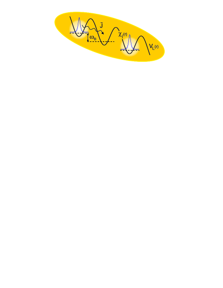
Figure 1: Impurities described by the localized Wannier functions $\chi_{j}(\mathbf{r})$ are trapped in the optical lattice potential $V_{L}(\mathbf{r})$ and immersed in a nearly uniform BEC. A tilt imposed on the periodic potential leads to the formation of a Wannier-Stark ladder (dotted lines) with levels separated by the Bloch frequency $\omega_{B}$. Inelastic scattering of Bogoliubov phonons results in a net atomic current across the tilted lattice. The current depends on the effective hopping $\tilde{J}$, the level separation $\omega_{B}$ and the effective relaxation time of the impurities.

In the present paper we study the dynamics of impurities immersed in a nearly uniform BEC, which in addition are trapped in an optical lattice potential [28, 29]. This setup has been considered in [30] by the present authors, however, we here motivate and develop the small polaron formalism in more detail and extend the results to the case of a tilted optical lattice potential, as illustrated in Fig. 1. In contrast to similar previously-studied systems, the presence of an optical lattice allows us to completely control the kinetic energy of the impurities. Crucially, for impurities in the lowest Bloch band of the optical lattice the kinetic energy is considerably reduced by increasing the depth of the lattice potential [28, 29]. As a consequence, it is possible to access the so-called strong-coupling regime [31], where the interaction energy due to the coupling between the impurity and the BEC is much larger than the kinetic energy of the impurity. This regime is particularly interesting since it involves incoherent and dissipative multi-phonon processes which have a profound effect on the transport properties of the impurities.

As a starting point we investigate the problem of static impurities based on the GP approximation and by means of a Bogoliubov description of the quantized excitations [26, 32]. The main part of the paper is based on small polaron theory [33, 34, 35], where the polaron is composed of an impurity dressed by a coherent state of Bogoliubov phonons. This formalism accounts in a natural way for the effects of the BEC background on the impurities and allows us to describe the BEC deformation around the impurity in terms of displacement operators. As a principal result, we obtain an extended Hubbard model [36, 37] for the impurities, which includes the hopping of polarons and the effective impurity-impurity interaction mediated by the BEC. Moreover, the microscopic model is particularly suitable for the investigation of the transport of impurities from first principles within the framework of a generalized master equation (GME) approach [38, 39, 40, 41].

The transport properties of the impurities are considered in two distinct setups. We first show that in a non-tilted optical lattice the Bogoliubov phonons induce a crossover from coherent to incoherent hopping as the BEC temperature increases [30]. In addition, we extend the results in [30] to the case of a tilted optical lattice (see Fig. 1). We demonstrate that the inelastic phonon scattering responsible for the incoherent hopping of the impurities also provides the necessary relaxation process required for the emergence of a net atomic current across the lattice [42]. In particular, we find that the dependence of the current on the lattice tilt changes from ohmic conductance to negative differential conductance (NDC) for sufficiently low BEC temperatures. So far, to our knowledge, NDC has only been observed in a non-degenerate mixture of ultra-cold ⁴⁰K and ⁸⁷Rb atoms [12] and in semiconductor superlattices [43, 44], where the voltage-current dependence is known to obey the Esaki–Tsu relation [45]. By exploiting the analogy with a solid state system we show that the transition from ohmic conductance to NDC is accurately described by a similar relation, which allows us to determine the effective relaxation time of the impurities as a function of the BEC temperature.

The implementation of our setup relies on recent experimental progress in the production of quantum degenerate atomic mixtures [6, 7, 8, 9] and their confinement in optical lattice potentials [10, 11]. As proposed in [46], the impurities in the optical lattice can be cooled to extremely low temperatures by exploiting the collisional interaction with the surrounding BEC. The tilt imposed on the lattice potential may be achieved either by accelerating the lattice [47] or superimposing an additional harmonic potential [12, 48].

An essential requirement for our model is that neither interactions with impurities nor the trapping potential confining the impurities impairs the ability of the BEC to sustain phonon-like excitations. The first condition limits the number of impurity atoms [10, 11, 49], and thus we assume that the filling factor of the lattice is much lower than one, whereas the second requirement can be met by using a species-specific optical lattice potential [50]. Unlike in the case of self-trapped impurities [22, 23, 24], we assume that the one-particle states of the impurities are not modified by the BEC, which can be achieved by sufficiently tight impurity trapping as shown in C.

The paper is organized as follows. In Section 2 we present our model. In Section 3, we motivate the small polaron formalism by considering the problem of static impurities based on the GP equation and within the framework of Bogoliubov theory. In Section 4, the full dynamics of the impurities is included. We develop the small polaron formalism in detail and derive an effective Hamiltonian for hopping impurities. In Section 5, the GME is used to investigate the transport properties of the impurity atoms. First, we discuss the crossover from coherent to incoherent hopping and subsequently study the dependence of a net atomic current across a tilted optical lattice on the system parameters. We discuss possible extensions of our model and conclude in Section 6. Throughout the paper we consider impurity hopping only along one single direction for notational convenience. However, the generalization to hopping along more than one direction is straightforward.

2 Model

The Hamiltonian of the system is composed of three parts $\hat{H}=\hat{H}_{B}+\hat{H}_{\chi}+\hat{H}_{I}$, where $\hat{H}_{B}$ is the Hamiltonian of the Bose-gas, $\hat{H}_{\chi}$ governs the dynamics of the impurity atoms and $\hat{H}_{I}$ describes the interactions between the impurities and the condensate atoms.

The Bose-gas is assumed to be at a temperature $T$ well below the critical temperature $T_{c}$, so that most of the atoms are in the Bose-condensed state. The boson-boson interaction is represented by a pseudo-potential $g\delta(\mathbf{r}-\mathbf{r}^{\prime})$, where the coupling constant $g>0$ depends on the s-wave scattering length of the condensate atoms. Accordingly, the grand canonical Hamiltonian $\hat{H}_{B}$ of the Bose-gas reads

$$\hat{H}_{B}=\int\mathrm{d}\mathbf{r}\,\hat{\psi}^{\dagger}(\mathbf{r})\left[\hat{H}_{0}-\mu_{b}\right]\hat{\psi}(\mathbf{r})+\frac{g}{2}\int\mathrm{d}\mathbf{r}\,\hat{\psi}^{\dagger}(\mathbf{r})\hat{\psi}^{\dagger}(\mathbf{r})\hat{\psi}(\mathbf{r})\hat{\psi}(\mathbf{r})\,,$$ (1)

where $\mu_{b}$ is the chemical potential and

$$\hat{H}_{0}=-\frac{\hbar^{2}}{2m_{b}}\nabla^{2}+V_{\mathrm{ext}}(\mathbf{r})$$ (2)

is the single-particle Hamiltonian of the non-interacting gas, with $m_{b}$ the mass of a boson and $V_{\mathrm{ext}}(\mathbf{r})$ is a shallow external trapping potential. The boson field operators $\hat{\psi}^{\dagger}(\mathbf{r})$ and $\hat{\psi}(\mathbf{r})$ create and annihilate an atom at position $\mathbf{r}$, respectively, and satisfy the bosonic commutation relations $[\hat{\psi}(\mathbf{r}),\hat{\psi}^{\dagger}(\mathbf{r}^{\prime})]=\delta(\mathbf{r}-\mathbf{r}^{\prime})$ and $[\hat{\psi}(\mathbf{r}),\hat{\psi}(\mathbf{r}^{\prime})]=[\hat{\psi}^{\dagger}(\mathbf{r}),\hat{\psi}^{\dagger}(\mathbf{r}^{\prime})]=0$.

To be specific we consider bosonic impurity atoms with mass $m_{a}$ loaded into an optical lattice, which are described by the impurity field operator $\hat{\chi}(\mathbf{r})$. The optical lattice potential for the impurities is of the form $V_{L}(\mathbf{r})=V_{x}\sin^{2}(kx)+V_{y}\sin^{2}(ky)+V_{z}\sin^{2}(kz)$, with the wave-vector $k=2\pi/\lambda$ and $\lambda$ the wavelength of the laser beams. The depth of the lattice $V_{\ell}$ ($\ell=x,y,z$) is determined by the intensity of the corresponding laser beam and conveniently measured in units of the recoil energy $E_{R}=\hbar^{2}k^{2}/2m_{a}$. Since we are interested in the strong-coupling regime we assume that the depth of the lattice exceeds several recoil energies. As a consequence, the impurity dynamics is accurately described in the tight-binding approximation by the Bose–Hubbard model [28, 29], where the mode-functions of the impurities $\chi_{j}(\mathbf{r})$ are Wannier functions of the lowest Bloch band localized at site $j$, satisfying the normalization condition $\int\mathrm{d}\mathbf{r}|\chi_{j}(\mathbf{r})|^{2}=1$. Accordingly, the impurity field operator is expanded as $\hat{\chi}(\mathbf{r})=\sum_{j}\chi_{j}(\mathbf{r})\hat{a}_{j}$ and the Bose–Hubbard Hamiltonian is given by

$$\hat{H}_{\chi}=-J\sum_{\langle i,j\rangle}\hat{a}^{\dagger}_{i}\hat{a}_{j}+\frac{1}{2}U\sum_{j}\hat{n}_{j}(\hat{n}_{j}-1)+\mu_{a}\sum_{j}\hat{n}_{j}+\hbar\omega_{B}\sum_{j}j\,\hat{n}_{j}\,,$$ (3)

where $\mu_{a}$ is the energy offset, $U$ is the on-site interaction strength, $J$ is the hopping matrix element between adjacent sites and $\langle i,j\rangle$ denotes the sum over nearest neighbours. The operators $\hat{a}^{\dagger}_{j}$ ($\hat{a}_{j}$) create (annihilate) an impurity at lattice site $j$ and satisfy the bosonic commutation relations $[\hat{a}_{i},\hat{a}^{\dagger}_{j}]=\delta_{i,j}$ and $[\hat{a}_{i},\hat{a}_{j}]=[\hat{a}^{\dagger}_{i},\hat{a}^{\dagger}_{j}]=0$, and $\hat{n}_{j}=\hat{a}^{\dagger}_{j}\hat{a}_{j}$ is the number operator. The last term in Eq. (3) was added to allow for a tilted lattice with the energy levels of the Wannier states $\chi_{j}(\mathbf{r})$ separated by Bloch frequency $\omega_{B}$, as shown in Fig. (1).

For the lattice depths considered in this paper it is possible to expand the potential wells about their minima and approximate the Wannier functions by harmonic oscillator ground states. The oscillation frequencies of the wells are $\omega_{\ell}=2\sqrt{E_{R}V_{\ell}}/\hbar$ and the spread of the mode-functions $\chi_{j}(\mathbf{r})$ is given by the harmonic oscillator length $\sigma_{\ell}=\sqrt{\hbar/m_{a}\omega_{\ell}}\,$. Explicitly, the Gaussian mode-function in one dimension reads

$$\chi_{j,\sigma}(x)=\big{(}\pi\sigma^{2}\big{)}^{-1/4}\exp\left[-(x-x_{j})^{2}/(2\sigma^{2})\right]\,,$$ (4)

where $x_{j}=aj$ with $a=\lambda/2$ being the lattice spacing. We note that the mode-functions $\chi_{j,\sigma}(\mathbf{r})$ are highly localized on a scale short compared to the lattice spacing $a$ since $\sigma_{\ell}/a=(V_{\ell}/E_{R})^{-1/4}/\pi\ll 1$ for sufficiently deep lattices. Consistency of the tight-binging model requires that excitations into the first excited Bloch band due to Landau-Zener tunneling or on-site interactions are negligible, i.e. $\omega_{B}\ll\omega_{\ell}$ and $1/2\,Un_{j}(n_{j}-1)\ll\hbar\omega_{\ell}$, with $n_{j}$ the occupation numbers. These inequalities are readily satisfied in practice.

The density-density interaction between the impurities and the Bose-gas atoms is again described by a pseudo-potential $\kappa\delta(\mathbf{r}-\mathbf{r}^{\prime})$, with $\kappa$ the coupling constant, and the interaction Hamiltonian is of the form

$$\hat{H}_{I}=\kappa\int\mathrm{d}\mathbf{r}\,\hat{\chi}^{\dagger}(\mathbf{r})\hat{\chi}(\mathbf{r})\hat{\psi}^{\dagger}(\mathbf{r})\hat{\psi}(\mathbf{r})\,.$$ (5)

We note that the effect of $\hat{H}_{B}$ and $\hat{H}_{I}$ dominate the dynamics of the system in the strong-coupling regime and hence the kinetic part in $\hat{H}_{\chi}$ can be treated as a perturbation.

3 Static impurities

In a first step we investigate the interaction of static impurities with the BEC, i.e. we neglect the hopping term in $\hat{H}_{\chi}$. We first derive a mean-field Hamiltonian based on the GP approximation and subsequently quantize the small-amplitude oscillations about the GP ground state using standard Bogoliubov theory [26, 32].

In the GP approximation, the bosonic field operator $\hat{\psi}(\mathbf{r})$ is replaced by the classical order parameter of the condensate $\psi(\mathbf{r})$. Accordingly, the impurities are described by the impurity density $\rho_{\chi}(\mathbf{r})=\langle\hat{\chi}^{\dagger}(\mathbf{r})\hat{\chi}(\mathbf{r})\rangle=\sum_{j}n_{j}|\chi_{j}(\mathbf{r})|^{2}$, where the average is taken over a fixed product state $|\Upsilon\rangle$ representing a set of static impurities, i.e. $|\Upsilon\rangle=\prod_{\{j\}}\hat{a}^{\dagger}_{j}|0\rangle$, with $\{j\}$ a set of occupied sites and $|0\rangle$ the impurity vacuum. We linearize the equation for $\psi(\mathbf{r})$ by considering small deviations $\vartheta(\mathbf{r})=\psi(\mathbf{r})-\psi_{0}(\mathbf{r})$ from the ground state of the condensate $\psi_{0}(\mathbf{r})$ in absence of impurities. This approach is valid provided that $|\vartheta(\mathbf{r})|/\psi_{0}(\mathbf{r})\ll 1$ and corresponds to an expansion of $\hat{H}_{B}+\hat{H_{I}}$ to second order in $\kappa$. Explicitly, by replacing $\hat{\psi}(\mathbf{r})$ with $\psi_{0}(\mathbf{r})+\vartheta(\mathbf{r})$ in $\hat{H}_{B}+\hat{H}_{I}$ we obtain the GP Hamiltonian $H_{GP}=H_{\psi_{0}}+H_{\vartheta}+H_{\mathrm{lin}}$ with

$$H_{\psi_{0}}=\int\mathrm{d}\mathbf{r}\left\{\psi_{0}^{\ast}(\mathbf{r})H_{0}\psi_{0}(\mathbf{r})-\mu_{b}|\psi_{0}(\mathbf{r})|^{2}+\frac{g}{2}|\psi_{0}(\mathbf{r})|^{4}\right\}+\kappa\int\mathrm{d}\mathbf{r}\,\rho_{\chi}(\mathbf{r})|\psi_{0}(\mathbf{r})|^{2}\,,$$ (6a)

$$H_{\vartheta} = \int\mathrm{d}\mathbf{r}\left\{\vartheta^{\ast}(\mathbf{r})\left[H_{0}-\mu_{b}+2g|\psi_{0}(\mathbf{r})|^{2}\right]\vartheta(\mathbf{r})\right\}$$ (6b)

$$\qquad\quad+\frac{g}{2}\int\mathrm{d}\mathbf{r}\left\{\vartheta^{\ast}(\mathbf{r})[\psi_{0}(\mathbf{r})]^{2}\vartheta^{\ast}(\mathbf{r})+\vartheta(\mathbf{r})[\psi_{0}^{\ast}(\mathbf{r})]^{2}\vartheta(\mathbf{r})\right\}\,,$$

$$H_{\mathrm{lin}}=\kappa\int\mathrm{d}\mathbf{r}\,\rho_{\chi}(\mathbf{r})\left[\psi_{0}(\mathbf{r})\vartheta^{\ast}(\mathbf{r})+\psi_{0}^{\ast}(\mathbf{r})\vartheta(\mathbf{r})\right]\,.$$ (6c)

In absence of impurities, i.e. for $\kappa=0$ and $\vartheta(\mathbf{r})$ identically zero, the stationary condition $\delta H_{GP}/\delta\psi_{0}^{\ast}(\mathbf{r})=0$ implies that $\psi_{0}(\mathbf{r})$ satisfies the time-independent GP equation

$$\left[H_{0}+g|\psi_{0}(\mathbf{r})|^{2}\right]\psi_{0}(\mathbf{r})=\mu_{b}\psi_{0}(\mathbf{r})\,.$$ (6g)

The deformed ground state of $H_{GP}$ due to the presence of impurities is found by imposing the stationary condition $\delta H_{GP}/\delta\vartheta^{\ast}(\mathbf{r})=0$ or equivalently

$$\left[H_{0}-\mu_{b}+2g|\psi_{0}(\mathbf{r})|^{2}\right]\vartheta(\mathbf{r})+g[\psi_{0}(\mathbf{r})]^{2}\vartheta^{\ast}(\mathbf{r})+\kappa\rho_{\chi}(\mathbf{r})\psi_{0}(\mathbf{r})=0\,,$$ (6h)

which is the Bogoliubov–de Gennes equation [26, 32] for the zero-frequency mode.

For the case of a homogeneous BEC, the effect of the impurities on the ground state of the condensate can be expressed in terms of Green’s functions [22, 23, 27]. If we assume for simplicity that both $\psi_{0}(\mathbf{r})$ and $\vartheta(\mathbf{r})$ are real then Eq. (6h) reduces to the modified Helmholtz equation

$$\left[\nabla^{2}-\left(\frac{2}{\xi}\right)^{2}\right]\vartheta(\mathbf{r})=\frac{2\kappa}{g\sqrt{n_{0}}\xi^{D}}\rho_{\chi}(\mathbf{r})\,,$$ (6i)

where $\xi=\hbar/\sqrt{m_{b}gn_{0}}$ is the healing length, $D$ is the number of spatial dimensions, and $n_{0}=|\psi_{0}|^{2}$ is the condensate density. The solution of Eq. (6i) is found to be [51]

$$\vartheta(\mathbf{r})=-\frac{\kappa}{g\sqrt{n_{0}}\xi^{D}}\int\mathrm{d}\mathbf{r}^{\prime}\,\mathcal{G}(\mathbf{r}-\mathbf{r}^{\prime})\rho_{\chi}(\mathbf{r}^{\prime})\,,$$ (6j)

where the Green’s functions are

$$\mathcal{G}_{\mathrm{1D}}(\mathbf{r}) =\frac{1}{2}\exp(-2|\mathbf{r}|/\xi)\,,$$ (6ka)

$$\mathcal{G}_{\mathrm{2D}}(\mathbf{r}) =\frac{1}{\pi}\mathrm{K}_{0}(2|\mathbf{r}|/\xi)\,,$$ (6kb)

$$\mathcal{G}_{\mathrm{3D}}(\mathbf{r}) =\frac{1}{2\pi}\frac{\exp(-2|\mathbf{r}|/\xi)}{|\mathbf{r}|/\xi}\,,$$ (6kc)

with $\mathrm{K}_{0}(x)$ the modified Bessel function of the second kind. Thus, independent of the dimension $D$ of the system, the BEC deformation induced by the impurities falls off exponentially on a length scale set by $\xi$, as illustrated in Fig. (2).

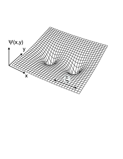
Figure 2: The order parameter $\psi(\mathbf{r})$ of a two-dimensional homogeneous condensate deformed by two highly localized impurities with $\kappa>0$ according to Eq. (6j). The deformation of the BEC results in an effective interaction potential $\mathcal{V}_{i,j}$ between the impurities at lattice sites $i$ and $j$. The range of the potential is characterized by the healing length $\xi$, which is comparable to the lattice spacing $a$ for realistic experimental parameters.

It follows from Eq. (6j) that for occupation numbers $n_{j}\sim 1$ the condition $|\vartheta(\mathbf{r})|/\psi_{0}(\mathbf{r})\ll 1$ is equivalent to

$$\alpha=\frac{|\kappa|}{g}\left(\frac{d}{\xi}\right)^{D}\ll 1\,,$$ (6kl)

with $d=n_{0}^{-1/D}$ the average separation of the condensate atoms. The generalization of this condition to the non-homogeneous case is $\alpha(\mathbf{r})=(|\kappa|/g)\,[d(\mathbf{r})/\xi(\mathbf{r})]^{D}\ll 1$ under the assumption that the BEC is nearly uniform. We note that $\alpha(\mathbf{r})\propto n_{0}(\mathbf{r})^{(D-2)/2}$, and hence $\alpha(\mathbf{r})$ diverges in 1D as $n_{0}(\mathbf{r})\rightarrow 0$, e.g. near the boundary of the condensate. However, this is consistent with the GP approach, which is no longer applicable in the dilute limit $\xi(\mathbf{r})/d(\mathbf{r})\ll 1$ of a 1D Bose-gas [26].

The change in energy of the BEC due to the impurities is found by inserting the formal solution for $\vartheta(\mathbf{r})$ in Eq. (6j) into $H_{GP}$. Provided that $\vartheta(\mathbf{r})$ satisfies Eq. (6h) the identity $H_{\mathrm{lin}}+2H_{\vartheta}=0$, or equivalently $H_{GP}=H_{\psi_{0}}+\frac{1}{2}H_{\mathrm{lin}}$, holds. Using the latter expression for $H_{GP}$ we find

$$H_{GP}=\sum_{j}\left(\bar{\mathcal{E}}-\mathcal{E}_{j}\right)n_{j}-\sum_{j}\mathcal{E}_{j}\,n_{j}\left(n_{j}-1\right)-\frac{1}{2}\sum_{i\neq j}\mathcal{V}_{i,j}\,n_{i}n_{j}\,,$$ (6km)

where $\bar{\mathcal{E}}=\kappa n_{0}$ is the first order contribution to the mean-field shift. In Eq. (6km) we have neglected constant terms which do not depend on the impurity configuration, i.e. contributions containing $\psi_{0}(\mathbf{r})$ only. The off-site interaction potential between the impurities is given by

$$\mathcal{V}_{i,j}=\frac{2\kappa^{2}}{g\xi^{D}}\int\mathrm{d}\mathbf{r}\,\mathrm{d}\mathbf{r}^{\prime}|\chi_{i}(\mathbf{r})|^{2}\mathcal{G}(\mathbf{r}-\mathbf{r}^{\prime})|\chi_{j}(\mathbf{r}^{\prime})|^{2}\,,$$ (6kn)

and $\mathcal{E}_{j}=\frac{1}{2}\mathcal{V}_{j,j}$ is the potential energy of an impurity, both resulting from the deformation of the condensate, as illustrated in Fig. (2).

In order to quantize the GP solution we consider small excitations $\hat{\zeta}(\mathbf{r})$ of the system, which obey bosonic commutation relations, around the static GP ground state $\psi_{0}(\mathbf{r})+\vartheta(\mathbf{r})$ of the condensate [26, 32]. This corresponds to an expansion of the bosonic field operator as $\hat{\psi}(\mathbf{r})=\psi_{0}(\mathbf{r})+\vartheta(\mathbf{r})+\hat{\zeta}(\mathbf{r})$. The Hamiltonian $\hat{H}_{\zeta}$ governing the evolution of $\hat{\zeta}(\mathbf{r})$ can be obtained by substituting $\vartheta(\mathbf{r})+\hat{\zeta}(\mathbf{r})$ for $\vartheta(\mathbf{r})$ in $H_{GP}$. By collecting the terms containing $\hat{\zeta}(\mathbf{r})$ and $\hat{\zeta}^{\dagger}(\mathbf{r})$ we find

$$\hat{H}_{\zeta} = \int\mathrm{d}\mathbf{r}\left\{\hat{\zeta}^{\dagger}(\mathbf{r})\left[H_{0}-\mu_{b}+2g|\psi_{0}(\mathbf{r})|^{2}\right]\hat{\zeta}(\mathbf{r})\right\}$$ (6ko)

$$\qquad\quad+\frac{g}{2}\int\mathrm{d}\mathbf{r}\left\{\hat{\zeta}^{\dagger}(\mathbf{r})[\psi_{0}(\mathbf{r})]^{2}\hat{\zeta}^{\dagger}(\mathbf{r})+\hat{\zeta}(\mathbf{r})[\psi_{0}^{\ast}(\mathbf{r})]^{2}\hat{\zeta}(\mathbf{r})\right\}\,,$$

where the linear terms in $\hat{\zeta}(\mathbf{r})$ and $\hat{\zeta}^{\dagger}(\mathbf{r})$ vanish identically since $\vartheta(\mathbf{r})$ satisfies Eq. (6h). The Hamiltonian $\hat{H}_{\zeta}$ in Eq. (6ko) can be diagonalized by the standard Bogoliubov transformation [26, 32]

$$\hat{\zeta}(\mathbf{r})=\sum_{\nu}\left[u_{\nu}(\mathbf{r})\hat{\beta}_{\nu}+v_{\nu}^{\ast}(\mathbf{r})\hat{\beta}^{\dagger}_{\nu}\right]\,.$$ (6kp)

Here, $u_{\nu}(\mathbf{r})$ and $v_{\nu}^{\ast}(\mathbf{r})$ are complex functions and the operators $\hat{\beta}^{\dagger}_{\nu}$ ($\hat{\beta}_{\nu}$) create (annihilate) a Bogoliubov quasi-particle, with quantum numbers $\nu$, and satisfy bosonic commutation relations. The Bogoliubov transformation in Eq. (6kp) reduces the Hamiltonian $\hat{H}_{\zeta}$ to a collection of noninteracting quasi-particles provided that the coefficients $u_{\nu}(\mathbf{r})$ and $v_{\nu}(\mathbf{r})$ obey the Bogoliubov–de Gennes equations [26, 32]

$$\eqalign{&\left[H_{0}-\mu_{b}+2g|\psi_{0}(\mathbf{r})|^{2}\right]u_{\nu}(\mathbf{r})+g[\psi_{0}(\mathbf{r})]^{2}v_{\nu}(\mathbf{r})=\hbar\omega_{\nu}u_{\nu}(\mathbf{r})\,,\\ &\left[H_{0}-\mu_{b}+2g|\psi_{0}(\mathbf{r})|^{2}\right]v_{\nu}(\mathbf{r})+g[\psi_{0}^{\ast}(\mathbf{r})]^{2}u_{\nu}(\mathbf{r})=-\hbar\omega_{\nu}v_{\nu}(\mathbf{r})\,,}$$ (6ks)

with the spectrum $\hbar\omega_{\nu}$. Under the condition that Eqs. (6ks) are satisfied one finds that $\hat{H}_{\zeta}$ takes the form $\hat{H}_{\zeta}=\sum_{\nu}\hbar\omega_{\nu}\hat{\beta}^{\dagger}_{\nu}\hat{\beta}_{\nu}$, where constant terms depending on $\psi_{0}(\mathbf{r})$ and $v_{\nu}(\mathbf{r})$ only were neglected .

Consequently, the total Hamiltonian $\hat{H}_{\mathrm{stat}}$ of the BEC and the static impurities is composed of three parts

$$\hat{H}_{\mathrm{stat}}=\hat{H}_{\zeta}+H_{GP}+\langle\hat{H}_{\chi}\rangle\,,$$ (6kt)

where $\hat{H}_{\zeta}$ governs the dynamics of the Bogoliubov quasi-particles and $H_{GP}$ is the GP ground state energy, which for the case of a homogeneous BEC takes the simple form in Eq. (6km). The third term $\langle\hat{H}_{\chi}\rangle$ represents the average value of $\hat{H}_{\chi}$ with respect to the fixed product state $|\Upsilon\rangle$ introduced earlier with $n_{j}$ impurities at each site $j$, giving explicitly

$$\langle\hat{H}_{\chi}\rangle=\frac{1}{2}U\sum_{j}n_{j}(n_{j}-1)+\mu_{a}\sum_{j}n_{j}+\hbar\omega_{B}\sum_{j}j\,n_{j}\,.$$ (6ku)

The ground state of the system corresponds to the Bogoliubov vacuum defined by $\hat{\beta}_{\nu}|\mathrm{vac}\rangle=0$.

4 Hopping impurities in the polaron picture

Given the Hamiltonian $\hat{H}_{\mathrm{stat}}$ derived in the previous section it is straightforward to determine the ground state energy for a set of static impurities. However, an analysis of the full dynamics of the impurities requires an alternative description in terms of polarons, i.e. impurities dressed by a coherent state of Bogoliubov quasi-particles. In this picture small polaron theory allows us, for example, to calculate the effective hopping matrix element for the impurities, which takes the BEC background into account.

Our approach is based on the observation that the Hamiltonian $\hat{H}_{\zeta}$ of the quantized excitations and consequently the Bogoliubov–de Gennes equations (6ks) are independent of $\rho_{\chi}(\mathbf{r})$. In other words, the effect of the impurities is only to shift the equilibrium position of the modes $\hat{\beta}_{\nu}$ without changing the spectrum $\hbar\omega_{\nu}$. Therefore it is possible to first expand the bosonic field operator as $\hat{\psi}(\mathbf{r})=\psi_{0}(\mathbf{r})+\hat{\vartheta}(\mathbf{r})$, with $\hat{\vartheta}(\mathbf{r})=\vartheta(\mathbf{r})+\hat{\zeta}(\mathbf{r})$, subsequently express $\hat{\vartheta}(\mathbf{r})$ in terms of Bogoliubov modes about the state $\psi_{0}(\mathbf{r})$ and finally shift their equilibrium positions in order to (approximately) minimize the total energy of the system.

Similarly to the case of static impurities, we first replace $\hat{\psi}(\mathbf{r})$ with $\psi_{0}(\mathbf{r})+\hat{\vartheta}(\mathbf{r})$ in $\hat{H}_{B}+\hat{H}_{I}$ to obtain the Hamiltonian $\hat{H}_{GP}=\hat{H}_{\psi_{0}}+\hat{H}_{\vartheta}+\hat{H}_{\mathrm{lin}}$ with

$$\hat{H}_{\psi_{0}}=\int\mathrm{d}\mathbf{r}\left\{\psi_{0}^{\ast}(\mathbf{r})H_{0}\psi_{0}(\mathbf{r})-\mu_{b}|\psi_{0}(\mathbf{r})|^{2}+\frac{g}{2}|\psi_{0}(\mathbf{r})|^{4}\right\}+\kappa\int\mathrm{d}\mathbf{r}\,\hat{\chi}^{\dagger}(\mathbf{r})\hat{\chi}(\mathbf{r})|\psi_{0}(\mathbf{r})|^{2}\,,$$ (6kva)

$$\hat{H}_{\vartheta} = \int\mathrm{d}\mathbf{r}\left\{\hat{\vartheta}^{\dagger}(\mathbf{r})\left[H_{0}-\mu_{b}+2g|\psi_{0}(\mathbf{r})|^{2}\right]\hat{\vartheta}(\mathbf{r})\right\}$$ (6kvb)

$$\qquad\quad+\frac{g}{2}\int\mathrm{d}\mathbf{r}\left\{\hat{\vartheta}^{\dagger}(\mathbf{r})[\psi_{0}(\mathbf{r})]^{2}\hat{\vartheta}^{\dagger}(\mathbf{r})+\hat{\vartheta}(\mathbf{r})[\psi_{0}^{\ast}(\mathbf{r})]^{2}\hat{\vartheta}(\mathbf{r})\right\}\,,$$

$$\hat{H}_{\mathrm{lin}}=\kappa\int\mathrm{d}\mathbf{r}\,\hat{\chi}^{\dagger}(\mathbf{r})\hat{\chi}(\mathbf{r})\left[\psi_{0}(\mathbf{r})\hat{\vartheta}^{\dagger}(\mathbf{r})+\psi_{0}^{\ast}(\mathbf{r})\hat{\vartheta}(\mathbf{r})\right]\,.$$ (6kvc)

We note that now $\hat{H}_{GP}$ contains the density operator $\hat{\chi}^{\dagger}(\mathbf{r})\hat{\chi}(\mathbf{r})$ instead of $\rho_{\chi}(\mathbf{r})$ in order to take into account the full dynamics of the impurities. The expansion of $\hat{\vartheta}(\mathbf{r})$ in terms of Bogoliubov modes reads

$$\hat{\vartheta}(\mathbf{r})=\sum_{\nu}\left[u_{\nu}(\mathbf{r})\hat{b}_{\nu}+v_{\nu}^{\ast}(\mathbf{r})\hat{b}^{\dagger}_{\nu}\right]\,,$$ (6kvw)

where the spectrum $\hbar\omega_{\nu}$ and coefficients $u_{\nu}(\mathbf{r})$ and $v_{\nu}(\mathbf{r})$ are determined by Eqs. (6ks). The bosonic operators $\hat{b}^{\dagger}_{\nu}$ ($\hat{b}_{\nu}$) create (annihilate) a Bogoliubov excitation around the ground state of the condensate $\psi_{0}(\mathbf{r})$ in absence of impurities, and thus, importantly, do not annihilate the vacuum $|\mathrm{vac}\rangle$ defined in the previous section, i.e. $\hat{b}_{\nu}|\mathrm{vac}\rangle\neq 0$. By substituting the expansion in Eq. (6kvw) for $\hat{\vartheta}(\mathbf{r})$ in the Hamiltonian $\hat{H}_{GP}$ and using the identity $\hat{\chi}^{\dagger}(\mathbf{r})\hat{\chi}(\mathbf{r})=\sum_{i,j}\chi^{\ast}_{i}(\mathbf{r})\chi_{j}(\mathbf{r})\hat{a}^{\dagger}_{i}\hat{a}_{j}$ we find that up to constant terms

$$\hat{H}_{\psi_{0}} = \sum_{i,j}\bar{\mathcal{E}}_{i,j}\,\hat{a}^{\dagger}_{i}\hat{a}_{j}\,,$$ (6kvxa)

$$\hat{H}_{\vartheta} = \sum_{\nu}\hbar\omega_{\nu}\hat{b}^{\dagger}_{\nu}\hat{b}_{\nu}\,,$$ (6kvxb)

$$\hat{H}_{\mathrm{lin}} = \sum_{i,j,\nu}\hbar\omega_{\nu}\left[M_{i,j,\nu}\hat{b}_{\nu}+M^{\ast}_{i,j,\nu}\hat{b}^{\dagger}_{\nu}\right]\hat{a}^{\dagger}_{i}\hat{a}_{j}\,,$$ (6kvxc)

with the matrix elements

$$\eqalign{\bar{\mathcal{E}}_{i,j}&=\kappa\int\mathrm{d}\mathbf{r}\,n_{0}(\mathbf{r})\chi^{\ast}_{i}(\mathbf{r})\chi_{j}(\mathbf{r})\,,\\ M_{i,j,\nu}&=\frac{\kappa}{\hbar\omega_{\nu}}\int\mathrm{d}\mathbf{r}\,\psi_{0}(\mathbf{r})[u_{\nu}(\mathbf{r})+v_{\nu}(\mathbf{r})]\chi^{\ast}_{i}(\mathbf{r})\chi_{j}(\mathbf{r})\,,}$$ (6kvxy)

where we assumed for simplicity that $\psi_{0}(\mathbf{r})$ is real. The non-local couplings $M_{i,j,\nu}$ and $\bar{\mathcal{E}}_{i,j}$ with $i\neq j$ resulting from the off-diagonal elements in $\hat{\chi}^{\dagger}(\mathbf{r})\hat{\chi}(\mathbf{r})$ are highly suppressed because the product of two mode-functions $\chi_{i}(\mathbf{r})$ and $\chi_{j}(\mathbf{r})$ with $i\neq j$ is exponentially small. As a consequence, the evolution of the BEC and the impurities, including the full impurity Hamiltonian $\hat{H}_{\chi}$, is accurately described by the Hubbard–Holstein Hamiltonian [33, 34, 35]

$$\hat{H}_{\mathrm{hol}}=\hat{H}_{\chi}+\sum_{j,\nu}\hbar\omega_{\nu}\left[M_{j,\nu}\hat{b}_{\nu}+M^{\ast}_{j,\nu}\hat{b}^{\dagger}_{\nu}\right]\hat{n}_{j}+\sum_{j}\bar{\mathcal{E}}_{j}\,\hat{n}_{j}+\sum_{\nu}\hbar\omega_{\nu}\hat{b}^{\dagger}_{\nu}\hat{b}_{\nu}\,,$$ (6kvxz)

where we discarded the non-local couplings and introduced $\bar{\mathcal{E}}_{j}=\bar{\mathcal{E}}_{j,j}$ and $M_{j,\nu}=M_{j,j,\nu}$.

Since we intend to treat the dynamics of the impurities as a perturbation we shift the operators $\hat{b}_{\nu}$ and $\hat{b}^{\dagger}_{\nu}$ in such a way that $\hat{H}_{\mathrm{hol}}$ in Eq. (6kvxz) is diagonal, i.e. the total energy of the system is exactly minimized, for the case $J=0$. This is achieved by the unitary Lang-Firsov transformation [34, 35]

$$\hat{U}=\exp\left[\sum_{j,\nu}\left(M^{\ast}_{j,\nu}\hat{b}^{\dagger}_{\nu}-M_{j,\nu}\hat{b}_{\nu}\right)\hat{n}_{j}\right]\,,$$ (6kvxaa)

from which it follows that by applying the Baker-Campbell-Hausdorff formula [52] $\hat{U}\hat{b}^{\dagger}_{\nu}\hat{U}^{\dagger}=\hat{b}^{\dagger}_{\nu}-M_{j,\nu}\hat{n}_{j}$, $\hat{U}\hat{n}_{j}\hat{U}^{\dagger}=\hat{n}_{j}$ and $\hat{U}\hat{a}^{\dagger}_{j}\hat{U}^{\dagger}=\hat{a}^{\dagger}_{j}\hat{X}^{\dagger}_{j}$, with

$$\hat{X}^{\dagger}_{j}=\exp\left[\sum_{\nu}\left(M^{\ast}_{j,\nu}\hat{b}^{\dagger}_{\nu}-M_{j,\nu}\hat{b}_{\nu}\right)\right]\,.$$ (6kvxab)

The operator $\hat{X}^{\dagger}_{j}$ is the sought after displacement operator that creates a coherent state of Bogoliubov quasi-particles, i.e. a condensate deformation around the impurity. As a result, the transformed Hamiltonian $\hat{H}_{LF}=\hat{U}\hat{H}_{\mathrm{hol}}\hat{U}^{\dagger}$ is given by

$$\hat{H}_{LF} = -J\sum_{\langle i,j\rangle}(\hat{X}_{i}\hat{a}_{i})^{\dagger}(\hat{X}_{j}\hat{a}_{j})+\frac{1}{2}\sum_{j}\tilde{U}_{j}\,\hat{n}_{j}(\hat{n}_{j}-1)$$ (6kvxac)

$$\qquad\quad+\sum_{j}\tilde{\mu}_{j}\,\hat{n}_{j}+\hbar\omega_{B}\sum_{j}j\,\hat{n}_{j}-\frac{1}{2}\sum_{i\neq j}V_{i,j}\,\hat{n}_{i}\hat{n}_{j}+\sum_{\nu}\hbar\omega_{\nu}\hat{b}^{\dagger}_{\nu}\hat{b}_{\nu}\,,$$

with the effective energy offset $\tilde{\mu}_{j}=\mu_{a}+\bar{\mathcal{E}}_{j}-E_{j}$, the effective on-site interaction strength $\tilde{U}_{j}=U-2E_{j}$, the interaction potential $V_{i,j}=\sum_{\nu}\hbar\omega_{\nu}\left(M_{i,\nu}M^{\ast}_{j,\nu}+M^{\ast}_{i,\nu}M_{j,\nu}\right)$, and $E_{j}=\frac{1}{2}V_{j,j}$ the so-called polaronic level shift [34, 35].

In the case of static impurities and, more generally, in the limit $\zeta=J/E_{j}\ll 1$, the polarons created by $\hat{a}^{\dagger}_{j}\hat{X}^{\dagger}_{j}$ are the appropriate quasi-particles. Consequently, the Hamiltonian in Eq. (6kvxac) describes the dynamics of hopping polarons according to an extended Hubbard model [36, 37] with an non-retarded interaction potential $V_{i,j}$. The contributions to $\hat{H}_{LF}$ are qualitatively the same as for static impurities, except for the additional hopping term. In the thermodynamic limit, the interaction potential $V_{i,j}$ and the polaronic level shift $E_{j}$ are identical, respectively, to their GP counterparts $\mathcal{V}_{i,j}$ and $\mathcal{E}_{j}$. The reason for the simple connection between GP theory and small polaron results is that both involve a linearization of the equations describing the condensate. It should be noted that the interaction potential $V_{i,j}$ and the polaronic level shift $E_{j}$ can also be obtained exactly from $\hat{H}_{\mathrm{hol}}$ by applying standard Rayleigh-Schrödinger perturbation theory up to second order in $\kappa$ since all higher order terms vanish. However, the merit of using the Lang-Firsov transformation lies in the fact that it yields a true many-body description of the state of the system, which would require a summation of perturbation terms to all orders in $\kappa$ [53].

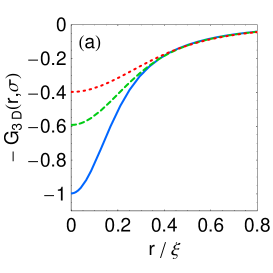
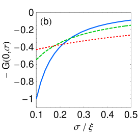
Figure 3: (a) The function $-\,G_{3D}(\mathbf{r},\sigma)$ plotted versus $\mathbf{r}$ for $\sigma/\xi=0.1$ (solid line), $\sigma/\xi=0.15$ (dashed line), $\sigma/\xi=0.2$ (dotted line). The potential $\mathcal{V}(\mathbf{r})\propto G_{3D}(\mathbf{r},\sigma)$ falls off on a scale set by $\xi$ and has an increasing depth $\mathcal{V}(0)$ with decreasing $\sigma$. (b) The function $-\,G(0,\sigma)$ plotted versus $\sigma$ for 3D (solid line), 2D (dashed line) and 1D (dotted line). The depth of the potential $\mathcal{V}(0)\propto G(0,\sigma)$ and $\mathcal{E}_{p}=\frac{1}{2}\mathcal{V}(0)$ depend strongly on $\sigma$ in 3D and only weakly in 2D and 1D. The relevant range of $\sigma$ can be estimated for deep lattices by $\sigma/\xi\approx(a/\xi)/[\pi(V_{\ell}/E_{R})^{1/4}]$.

We gain qualitative and quantitative insight into the dependence of the quantities in Eq. (6kvxac) on the system parameters by considering the specific case of a homogeneous BEC with the total Hamiltonian

$$\hat{H}_{LF} = -J\sum_{\langle i,j\rangle}(\hat{X}_{i}\hat{a}_{i})^{\dagger}(\hat{X}_{j}\hat{a}_{j})+\frac{1}{2}\tilde{U}\sum_{j}\hat{n}_{j}(\hat{n}_{j}-1)$$ (6kvxad)

$$\qquad\quad+\tilde{\mu}\sum_{j}\hat{n}_{j}+\hbar\omega_{B}\sum_{j}j\,\hat{n}_{j}-\frac{1}{2}\sum_{i\neq j}V_{i,j}\,\hat{n}_{i}\hat{n}_{j}+\sum_{\mathbf{q}}\hbar\omega_{\mathbf{q}}\hat{b}^{\dagger}_{\mathbf{q}}\hat{b}_{\mathbf{q}}\,,$$

with the energy offset $\tilde{\mu}=\mu_{a}+\kappa n_{0}-E_{p}$, the on-site interaction strength $\tilde{U}=U-2E_{p}$, the polaronic level shift $E_{j}\equiv E_{p}$ and the phonon momentum $\mathbf{q}$. For a homogeneous BEC the Bogoliubov coefficients are of the form $u_{\mathbf{q}}(\mathbf{r})=u_{\mathbf{q}}\exp(\mathrm{i}\mathbf{q}\cdot\mathbf{r})$ and $v_{\mathbf{q}}(\mathbf{r})=v_{\mathbf{q}}\exp(\mathrm{i}\mathbf{q}\cdot\mathbf{r})$ with [26, 32]

$$u_{\mathbf{q}}=\frac{1}{\sqrt{2\Omega}}\bigg{(}\frac{\varepsilon_{\mathbf{q}}+gn_{0}}{\hbar\omega_{\mathbf{q}}}+1\bigg{)}^{1/2}\,\,\mbox{and}\quad v_{\mathbf{q}}=-\frac{1}{\sqrt{2\Omega}}\bigg{(}\frac{\varepsilon_{\mathbf{q}}+gn_{0}}{\hbar\omega_{\mathbf{q}}}-1\bigg{)}^{1/2}\!.$$ (6kvxae)

Here, $\varepsilon_{\mathbf{q}}=(\hbar\mathbf{q})^{2}/2m_{b}$ is the free particle energy, $\hbar\omega_{\mathbf{q}}=\sqrt{\varepsilon_{\mathbf{q}}(\varepsilon_{\mathbf{q}}+2gn_{0})}$ is the Bogoliubov dispersion relation and $\Omega$ is the quantization volume. The corresponding matrix elements are found to be

$$M_{j,\mathbf{q}}=\kappa\sqrt{\frac{n_{0}\varepsilon_{\mathbf{q}}}{\left(\hbar\omega_{\mathbf{q}}\right)^{3}}}f_{j}(\mathbf{q})\,,$$ (6kvxaf)

where

$$f_{j}(\mathbf{q})=\frac{1}{\sqrt{\Omega}}\int\mathrm{d}\mathbf{r}|\chi_{j}(\mathbf{r})|^{2}\exp(\mathrm{i}\mathbf{q}\cdot\mathbf{r})\,.$$ (6kvxag)

For the Gaussian mode-function $\chi_{j,\sigma}(\mathbf{r})$ in Eq. (4) the factor $f_{j}(\mathbf{q})$ takes the simple form

$$f_{j}(\mathbf{q})=\frac{1}{\sqrt{\Omega}}\prod_{\ell}\exp\left(-q_{\ell}^{2}\sigma_{\ell}^{2}/4\right)\exp\left(\mathrm{i}\mathbf{q}\cdot\mathbf{r}_{j}\right)\,.$$ (6kvxah)

The $\mathbf{q}$-dependence of the impurity-phonon coupling is $M_{j,\mathbf{q}}\propto f_{j}(\mathbf{q})/\sqrt{|\mathbf{q}|}$ in the long wavelength limit $|\mathbf{q}|\ll 1/\xi$, which corresponds to a coupling to acoustic phonons in a solid state system [35], whereas in the free particle regime $|\mathbf{q}|\gg 1/\xi$ we have $M_{j,\mathbf{q}}\propto f_{j}(\mathbf{q})/\mathbf{q}^{2}$.

The potential $V_{i,j}$ and the polaronic level shift $E_{p}$ reduce to a sum over all momenta $\mathbf{q}$ and can be evaluated in the thermodynamic limit $\Omega^{-1}\sum_{\mathbf{q}}\!\rightarrow\!(2\pi)^{-D}\int\!\mathrm{d}\mathbf{q}$ where $V_{i,j}\rightarrow\mathcal{V}_{i,j}$. In particular, for the Gaussian mode-functions $\chi_{j,\sigma}(\mathbf{r})$ one finds

$$\mathcal{V}_{i,j}=\frac{2\kappa^{2}}{g\xi^{D}}\,G(\mathbf{r}_{i}-\mathbf{r}_{j},\sigma)\,,$$ (6kvxai)

where the functions $G(\mathbf{r},\sigma)$ are defined in A and plotted in Fig. 3a for a three-dimensional system. It follows from the definition of $G(\mathbf{r},0)$ that $\mathcal{G}(\mathbf{r})\equiv G(\mathbf{r},0)$, and hence the shape of the potential is determined by the Green’s function $\mathcal{G}(\mathbf{r})$ in the limit $\sigma\ll\xi$. The $\sigma$-dependence of $G(0,\sigma)$, which determines the depth of the interaction potential $\mathcal{V}_{i,j}$ and the level shift $\mathcal{E}_{p}=\frac{1}{2}\mathcal{V}_{j,j}$, is shown in Fig. 3b. The range of the potential, characterized by the healing length $\xi$, is comparable to the lattice spacing $a$ for realistic experimental parameters, and hence the off-site terms $V_{j,j+1}$ are non-negligible. In particular, as shown in [30, 54], the off-site interactions can lead to the aggregation of polarons on adjacent lattice sites into stable clusters, which are not prone to loss from three-body inelastic collisions.

5 Transport

The coupling to the Bogoliubov phonons via the operators $\hat{X}^{\dagger}_{j}$ and $\hat{X}_{j}$ changes the transport properties of the impurities notably. Since we assume the filling factor of the lattice to be much lower than one we can investigate the transport properties by considering a single polaron with the Hamiltonian $\hat{h}_{0}+\hat{h}_{I}$ given by

$$\hat{h}_{0} =\hbar\omega_{B}\sum_{j}j\,\hat{n}_{j}+\sum_{\mathbf{q}}\hbar\omega_{\mathbf{q}}\hat{b}^{\dagger}_{\mathbf{q}}\hat{b}_{\mathbf{q}}\,,$$ (6kvxaj)

$$\hat{h}_{I} =-J\sum_{\langle i,j\rangle}(\hat{X}_{i}\hat{a}_{i})^{\dagger}(\hat{X}_{j}\hat{a}_{j})\,.$$ (6kvxak)

To start we investigate the crossover from coherent to diffusive hopping [33, 35] in a non-tilted lattice ($\omega_{B}=0$) and then extend the result to a tilted lattice ($\omega_{B}\neq 0$) to demonstrate the emergence of a net atomic current across the lattice [42] due to energy dissipation into the BEC.

5.1 Coherent versus incoherent transport

We first consider coherent hopping of polarons at small BEC temperatures $k_{B}T\ll E_{p}$, where incoherent phonon scattering is highly suppressed. In the strong-coupling regime $\zeta=J/E_{j}\ll 1$, and hence the hopping term in Eq. (6kvxak) can be treated as a perturbation. The degeneracy of the Wannier states requires a change into the Bloch basis

$$|\mathbf{k}\rangle=\frac{1}{\sqrt{N}}\sum_{j}\exp(\mathrm{i}\mathbf{k}\cdot\mathbf{r}_{j})\,\hat{a}^{\dagger}_{j}|0\rangle\,,$$ (6kvxal)

with $\mathbf{k}$ the quasi-momentum and $N$ the number of lattice sites. Applying standard perturbation theory in the Bloch basis and describing the state of the system by $|\mathbf{k},\{N_{\mathbf{q}}\}\rangle$, where $\{N_{\mathbf{q}}\}$ is the phonon configuration with phonon occupation numbers $N_{\mathbf{q}}$, we find the polaron energy up to first order in $\zeta$

$$E(\mathbf{k})=\tilde{\mu}_{a}-2\tilde{J}\cos(\mathbf{k}\!\cdot\!\mathbf{a})\,,$$ (6kvxam)

where we defined the effective hopping $\tilde{J}=J\sum_{\mathbf{q}}\langle N_{\mathbf{q}}|\hat{X}^{\dagger}_{j}\hat{X}_{j+1}|N_{\mathbf{q}}\rangle$ and $\mathbf{a}$ is the position vector connecting two nearest neighbor sites. In particular, for the case of a thermal phonon distribution with occupation numbers $N_{\mathbf{q}}=(\textrm{e}^{\hbar\omega_{\mathbf{q}}/k_{B}T}-1)^{-1}$ the effective hopping is [33, 34, 35]

$$\tilde{J}=J\,\exp\Big{\{}-\sum_{\mathbf{q}\neq 0}|M_{0,\mathbf{q}}|^{2}\left[1-\cos(\mathbf{q}\!\cdot\!\mathbf{a})\right]\left(2N_{\mathbf{q}}+1\right)\Big{\}}\,.$$ (6kvxan)

Thus, the hopping bandwidth of the polaron band is highly suppressed with increasing coupling $\kappa$ and temperature $T$.

At high temperatures $E_{p}\ll k_{B}T\ll k_{B}T_{c}$ inelastic scattering, in which phonons are emitted and absorbed, becomes dominant, and thus the transport of impurities through the lattice changes from being purely coherent to incoherent. While matrix elements $\langle\{N_{\mathbf{q}}\}|\hat{X}^{\dagger}_{j}\hat{X}_{j+1}|\{N_{\mathbf{q}}\}^{\prime}\rangle$ involving two different phonon configurations $\{N_{\mathbf{q}}\}$ and $\{N_{\mathbf{q}}\}^{\prime}$ vanish at zero temperature they can take non-zero values for $T>0$. The condition for energy and momentum conservation during a hopping event implies that incoherent hopping is dominated by a three-phonon process that involves phonons with a linear dispersion $\hbar\omega_{\mathbf{q}}=\hbar c|\mathbf{q}|$, where $c\sim\sqrt{gn_{0}/m_{b}}$ is the speed of sound. This process is reminiscent of the well-known Beliaev decay of phonons [26].

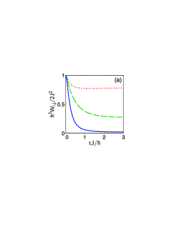
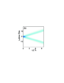
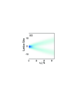
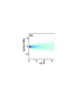
Figure 4: Coherent and diffusive hopping in a one-dimensional system: (a) The memory function $\hbar^{2}W_{i,j}(t)/(2J^{2})$ plotted versus time for $k_{B}T=0$ (dotted line), $k_{B}T=5E_{p}$ (dashed line) and $k_{B}T=15E_{p}$ (solid line). The memory function drops off rapidly for $k_{B}T\gg E_{p}$, indicating the dominance of incoherent hopping. (b) – (d) The evolution of the occupation probabilities $P_{j}(t)$ of a single impurity initially localized at site $j=0$ according to the GME with the memory functions in (a). (b) For small temperatures $k_{B}T\ll E_{p}$ the hopping is coherent with two wave-packets moving away from $j=0$. (d) For high temperatures $k_{B}T\gg E_{p}$ the inelastic scattering of phonons results in a diffusive motion of the impurity, where the probability $P_{j}(t)$ remains peaked at $j=0$. The lattice with spacing $a=395$nm and $J=2.45\times 10^{-2}E_{R}$ contains a single ⁴¹K atom. The BEC with $d=200$nm and $\xi=652$nm consists of ⁸⁷Rb atoms; $\kappa/g=2.58$, $E_{p}/k_{B}\approx 10$nK and $J/\hbar\approx 1.2$kHz.

We investigate the incoherent transport properties by using a generalized master equation (GME) [38] for the site occupation probabilities $P_{j}(t)$ of the impurity. This formalism has been applied to the transfer of excitons in the presence of electron-phonon coupling [39, 40] and is based on the Nakajima-Zwanzig projection method [41]. The generalized master equation is of the form

$$\frac{\partial P_{i}(t)}{\partial t}=\int_{0}^{t}\!\mathrm{d}s\,\sum_{j}W_{i,j}(s)\big{[}P_{j}(t-s)-P_{i}(t-s)\big{]}\,,$$ (6kvxao)

where the effect of the condensate is encoded in the memory functions $W_{i,j}(s)$. As shown in B the memory function to second order in $\zeta$ is given by

$$W_{i,j}(s) = \;2\delta_{j,i\pm 1}\Bigg{(}\frac{J}{\hbar}\Bigg{)}^{2}\mathrm{Re}\Bigg{[}\exp\Big{\{}\!-2\sum_{\mathbf{q}\neq 0}|M_{0,\mathbf{q}}|^{2}[1-\cos(\mathbf{q}\cdot\mathbf{a})]$$ (6kvxap)

$$\qquad\times\,[(N_{\mathbf{q}}+1)(1-\textrm{e}^{\mathrm{i}\omega_{\mathbf{q}}s})+N_{\mathbf{q}}(1-\textrm{e}^{-\mathrm{i}\omega_{\mathbf{q}}s})]\Big{\}}\exp(\pm\mathrm{i}\omega_{B}s)\Bigg{]}\,.$$

In the case $\omega_{B}=0$, the nontrivial part of $W_{i,j}(s)$ takes the values $2(J/\hbar)^{2}$ at $s=0$ and $2(\tilde{J}/\hbar)^{2}$ in the limit $s\rightarrow\infty$ due to the cancellation of highly oscillating terms, as shown in Fig. 4a.

In the regime $k_{B}T\ll E_{p}$, the effective hopping $\tilde{J}$ is comparable to $J$ and the memory function $W_{i,j}$ is well approximated by $2(\tilde{J}/\hbar)^{2}\Theta(s)$, with $\Theta(s)$ the Heaviside step function, and thus describes purely coherent hopping. In the regime $E_{p}\ll k_{B}T\ll k_{B}T_{c}$, processes involving thermal phonons become dominant and coherent hopping is highly suppressed, i.e. $\tilde{J}\ll J$. In this case the memory function $W_{i,j}$ drops off sufficiently fast for the Markov approximation to be valid, as illustrated in Fig. 4a. More precisely, one can replace $P_{j}(t-s)$ by $P_{j}(t)$ in Eq. (6kvxao) and after intergration over $s$ the GME reduces to the standard Pauli master equation

$$\frac{\partial P_{i}(t)}{\partial t}=\sum_{j}w_{i,j}\big{[}P_{j}(t)-P_{i}(t)\big{]}\,,$$ (6kvxaq)

where the hopping rates $w_{i,j}$ are given by

$$w_{i,j}=\int_{0}^{\infty}\!\mathrm{d}s\big{[}W_{i,j}(s)-\lim_{t\rightarrow\infty}W_{i,j}(t)\big{]}\,.$$ (6kvxar)

The Pauli master equation describes purely incoherent hopping with a thermally activated hopping rate $w_{i,j}$ [33, 35].

The evolution of an initially localized impurity at different temperatures $T$ for a one-dimensional ⁴¹K – ⁸⁷Rb system [8] is shown in Figs. 4b – 4d, which were obtained by numerically solving the GME with the memory function $W_{i,j}(s)$ in Eq. (6kvxap). It can be seen that for small temperatures $k_{B}T\ll E_{p}$ the hopping is coherent with two wave-packets moving away from the initial position of the impurity atom. In contrast, for high temperatures $k_{B}T\gg E_{p}$ inelastic scattering of phonons results in a diffusive motion of the impurity, where the probability $P_{j}(t)$ remains peaked at the initial position of the impurity.

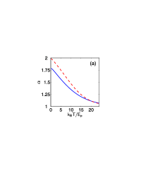
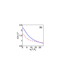
Figure 5: Analysis of the mean-square displacement $\overline{l^{2}}(t)=\sum_{l}l^{2}P_{l}(t)$, obtained from the evolution of an initially localized impurity in a one-dimensional system for the time $t_{\mathrm{evol}}=10\,\hbar/J$ according to the GME. The mean-squared displacement was assumed to be of the form $\overline{l^{2}}(t)=A\,t^{\alpha}$. (a) The exponent $\alpha$ versus temperature $T$ for the full evolution time (solid line) and the period $t_{\mathrm{evol}}/2$ to $t_{\mathrm{evol}}$ (dashed line). The drop from $\alpha\approx 2$ at zero temperature to $\alpha\approx 1$ at high temperatures $k_{B}T\gg E_{p}$ clearly indicates the crossover from coherent to diffusive transport. (b) The prefactor $A$ in units of $(J/\hbar)^{\alpha}$ versus temperature $T$ for the full evolution time (solid line) and the period $t_{\mathrm{evol}}/2$ to $t_{\mathrm{evol}}$ (dashed line). The system parameters are the same as for Fig. 4.

This crossover from coherent to diffusive hopping can be quantitatively analyzed by considering the mean-squared displacement of the impurity, $\overline{l^{2}}(t)=\sum_{l}l^{2}P_{l}(t)$, which we assume to be of the form $\overline{l^{2}}(t)=A\,t^{\alpha}$. The exponent $\alpha$ takes the value $\alpha=2$ for a purely coherent process, whereas $\alpha=1$ for diffusive hopping. Figure (5) shows $\alpha$ and $A$ in units of $(J/\hbar)^{\alpha}$ as functions of the BEC temperature $T$, which were obtained from the evolution (according to the GME) of an impurity initially localized at $j=0$. We see that the exponent $\alpha$ drops from $\alpha\approx 2$ at zero temperature to $\alpha\approx 1$ at high temperatures $k_{B}T\gg E_{p}$, thereby clearly indicating the crossover from coherent to diffusive transport. We note that the transition from coherent to diffusive hopping takes place in a temperature regime accessible to experimental study and therefore, importantly, may be observable.

5.2 Atomic current across a tilted lattice

The inelastic phonon scattering responsible for the incoherent hopping of the impurities also provides the necessary relaxation process required for the emergence of a net atomic current across a tilted optical lattice. This is in contrast to coherent Bloch oscillations, which occur in an optical lattice system in absence of incoherent relaxation effects or dephasing [47]. As pointed out in [42], the dependence of the atomic current on the lattice tilt $\hbar\omega_{B}$ changes from ohmic conductance to NDC in agreement with the theoretical model for electron transport introduced by Esaki and Tsu [45].

To demonstrate the emergence of a net atomic current, and, in particular, to show that impurities exhibit NDC, we consider the evolution of a localized impurity atom in a one-dimensional system. With the impurity initially at site $j=0$ we determine its average position $x_{d}=\sum_{j}aj\,P_{j}(t_{d})$ after a fixed drift time $t_{d}$ of the order of $\hbar/J$. This allows us to determine the drift velocity $v_{d}=x_{d}/t_{d}$ as a function of the lattice tilt $\hbar\omega_{B}$ and the temperature $T$ of the BEC. In analogy with a solid state system, the drift velocity $v_{d}$ and the lattice tilt $\hbar\omega_{B}$ correspond to the current and voltage, respectively.

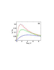
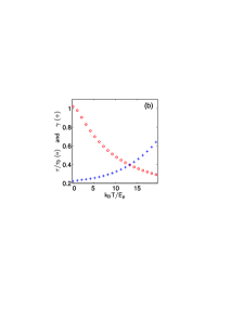
Figure 6: Current-voltage relation for a one-dimensional system: (a) The drift velocity $v_{d}$ in units of $v_{0}=Ja/\hbar$ as a function of the lattice tilt $\hbar\omega_{B}/J$ for temperatures $k_{B}T=0\;(+)$, $k_{B}T=5E_{p}\;(\circ)$ and $k_{B}T=15E_{p}\;(\times)$ according to the GME and the best fit of the Esaki–Tsu-type relation in Eq. (6kvxas) (dotted lines). The dependence of the current on the tilt changes from ohmic conductance $v_{d}\sim\hbar\omega_{B}$ to negative differential conductance $v_{d}\sim 1/(\hbar\omega_{B})$. (b) The relaxation time $\tau\;(\circ)$ in units of $\tau_{0}=\hbar/gn_{0}$ and the prefactor $\gamma\;(+)$ yielding the best fit of the Esaki–Tsu-type relation to the numerical results. The relaxation time $\tau$ of the impurities decreases with increasing BEC temperature $T$ and the prefactor $\gamma$ varies only slightly since the exponential temperature dependence of the current is accounted for by $\tilde{v}_{0}$. The system parameters are the same as for Fig. 4.

Figure 6a shows the voltage-current relation at different temperatures $T$, which was obtained by numerically solving the GME with the memory function in Eq. (6kvxap). We see that for a small lattice tilt the system exhibits ohmic behavior $v_{d}\sim\hbar\omega_{B}$, whereas for a large lattice tilt the current decreases with increasing voltage as $v_{d}\sim 1/(\hbar\omega_{B})$, i.e. the impurities feature NDC.

Following [42] we describe the voltage-current relation for the impurities by an Esaki–Tsu-type relation

$$v_{d}=2\gamma\tilde{v}_{0}\,\frac{\omega_{B}\tau}{1+(\omega_{B}\tau)^{2}}\,,$$ (6kvxas)

where $\tilde{v}_{0}=\tilde{J}a/\hbar$ the characteristic drift velocity, $\tau$ the effective relaxation time of the impurities and $\gamma$ a dimensionless prefactor. Fitting the Esaki–Tsu-type relation in Eq. (6kvxas) to the numerical data allows us to extract the parameters $\tau$ and $\gamma$, both depending on the BEC temperature. As can be seen in Fig. 6b, the effective relaxation time $\tau$ decreases with increasing BEC temperature $T$ and is of the order of $\tau_{0}=\hbar/(gn_{0})$. The significance of $1/\tau$ is that of an average collision rate between the impurities and Bogoliubov excitations, which would allow us, for example, to formulate the problem of transport in terms of a classical Boltzmann equation for the distribution function of the impurities [35]. The prefactor $\gamma$ varies only slightly since the exponential dependence of the current on the temperature is accounted for by $\tilde{v}_{0}$. We note that independently of $\omega_{B}\tau$ the maximum drift velocity is given by $\gamma\,\tilde{v}_{0}$.

The Esaki–Tsu-type relation in Eq. (6kvxas) reflects the competition between coherent and incoherent, dissipative processes. In the collision dominated regime $\omega_{B}\tau\ll 1$, inelastic scattering with phonons destroys Bloch oscillations, whereas in the collisionless regime $\omega_{B}\tau\gg 1$ the evolution of the impurities is mainly coherent, i.e. Bloch oscillations of the impurities lead to a suppression of the net current. The crossover between the two regimes is most pronounced at zero temperature, where $\tilde{J}$ is comparable to $J$. However, the change from ohmic to negative differential conductance is identifiable even at finite temperatures and thus should be observable in an experimental setup similar to the one used in [12].

6 Conclusion

We have studied the transport of impurity atoms in the strong-coupling regime, where the interaction energy due to the coupling between the BEC and the impurities dominates their dynamics. Within this regime, we have formulated an extended Hubbard model describing the impurities in terms of polarons, i.e. impurities dressed by a coherent state of Bogoliubov phonons. The model accommodates hopping of polarons and the effective off-site impurity-impurity interaction mediated by the BEC.

Based on the extended Hubbard model we have shown from first principles that inelastic phonon scattering results in a crossover from coherent to incoherent hopping and leads to the emergence of a net atomic current across a tilted optical lattice. In particular, we have found that the dependence of the current on the lattice tilt changes from ohmic conductance to negative differential conductance for sufficiently low BEC temperatures. Notably, this transition is accurately described by an Esaki–Tsu-type relation with the effective relaxation time of the impurities as a temperature-dependent parameter.

Using the techniques introduced in this paper, qualitatively similar phenomena can also be shown to occur for fermionic impurities and, moreover, for impurities of different species [55]. For instance, in the case of two impurity species $A$ and $B$ with the couplings $\kappa_{A}>0$ and $\kappa_{B}<0$, respectively, the effective off-site impurity-impurity interaction is attractive for the same species, but repulsive for different species. In either case, observation of the phenomena reported in this paper lies within the reach of current experiments, which may give new insight into the interplay between coherent, incoherent and dissipative processes in many-body systems.

Appendix A Definition of the functions $G(\mathbf{r},\sigma)$

The function $G(\mathbf{r},\sigma)$, which are a generalization of the Green’s functions $\mathcal{G}(\mathbf{r})$ for $\sigma>0$, are defined by

$$G_{\mathrm{1D}}(\mathbf{r},\sigma)=\frac{1}{\pi}\int_{-\infty}^{\infty}\mathrm{d}y\,\frac{\cos\left(y|\mathbf{r}|/\xi\right)}{y^{2}+4}\exp\left[-\frac{1}{2}\,y^{2}\left(\frac{\sigma}{\xi}\right)^{2}\right]\,,$$ (6kvxat)

$$G_{\mathrm{2D}}(\mathbf{r},\sigma)=\frac{1}{\pi}\int_{0}^{\infty}\mathrm{d}y\,y\,\frac{\mathrm{J}_{0}\!\left(y|\mathbf{r}|/\xi\right)}{y^{2}+4}\exp\left[-\frac{1}{2}\,y^{2}\left(\frac{\sigma}{\xi}\right)^{2}\right]\,,$$ (6kvxau)

where $\mathrm{J}_{0}(x)$ is the Bessel function of the first kind.

$$G_{\mathrm{3D}}(\mathbf{r},\sigma)=\frac{1}{\pi^{2}}\int_{0}^{\infty}\mathrm{d}y\,y^{2}\,\frac{\mathrm{j}_{0}\!\left(y|\mathbf{r}|/\xi\right)}{y^{2}+4}\exp\left[-\frac{1}{2}\,y^{2}\left(\frac{\sigma}{\xi}\right)^{2}\right]\,,$$ (6kvxav)

where $\mathrm{j}_{0}(x)=\sin(x)/x$ is the spherical Bessel function of the first kind. For the special case $\mathbf{r}=0$ we have with $z=\sqrt{2}\,\sigma/\xi$

$$G_{\mathrm{1D}}(0,\sigma) =\frac{1}{2}\exp(z^{2})\,\mathrm{erfc}(z)$$ (6kvxaw)

$$G_{\mathrm{2D}}(0,\sigma) =-\frac{1}{2\pi}\exp(z^{2})\,\mathrm{Ei}(-z^{2})$$ (6kvxax)

$$G_{\mathrm{3D}}(0,\sigma) =\frac{1}{\pi}\left[\frac{1}{\sqrt{\pi}z}-\exp(z^{2})\,\mathrm{erfc}(z)\right]$$ (6kvxay)

where $\mathrm{erfc}(x)$ is the complementary error function and $\mathrm{Ei}(x)$ is the exponential integral [56].

Appendix B Derivation of the GME

The Hamiltonian for the single impurity and the BEC is

$$\hat{h}_{0} =\hbar\omega_{B}\sum_{j}j\,\hat{n}_{j}+\sum_{\mathbf{q}}\hbar\omega_{\mathbf{q}}\hat{b}^{\dagger}_{\mathbf{q}}\hat{b}_{\mathbf{q}}$$

$$\hat{h}_{I} =-J\sum_{\langle i,j\rangle}(\hat{X}_{i}\hat{a}_{i})^{\dagger}(\hat{X}_{j}\hat{a}_{j})\,,$$

where $\hat{h}_{0}$ is the unperturbed Hamiltonian and $\hat{h}_{I}$ is treated as a perturbation in the strong-coupling regime $\zeta\ll 1$.

Starting point of the derivation of the GME is the Liouville-von Neumann equation [38]

$$\frac{\partial\hat{\rho}(t)}{\partial t}=\mathcal{L}\hat{\rho}(t)\,,$$ (6kvxaz)

where $\hat{\rho}(t)$ is the density matrix of the system expressed in the eigenbasis of $\hat{h}_{0}$. The Liouville operator $\mathcal{L}$ is defined by $\mathcal{L}=\mathcal{L}_{0}+\mathcal{L}_{I}$, with $\mathcal{L}_{0}=-\mathrm{i}/\hbar\,[\hat{h}_{0},\,\cdot\,]$ and $\mathcal{L}_{I}=-\mathrm{i}/\hbar\,[\hat{h}_{I},\,\cdot\,]$. The density matrix $\hat{\rho}(t)$ is decomposed as $\hat{\rho}(t)=\mathcal{P}\hat{\rho}(t)+\mathcal{Q}\hat{\rho}(t)$, where $\mathcal{P}$ is the projection operator on the relevant part of $\hat{\rho}(t)$ and $\mathcal{Q}=1-\mathcal{P}$ the complementary projection operator to $\mathcal{P}$. The time evolution of the relevant part $\mathcal{P}\hat{\rho}(t)$ is governed by the Nakajima-Zwanzig equation [41]

$$\frac{\partial}{\partial t}\mathcal{P}\hat{\rho}(t)=\mathcal{P}\mathcal{L}\mathcal{P}\hat{\rho}(t)+\!\int_{0}^{t}\!\mathrm{d}s\,\mathcal{P}\mathcal{L}\textrm{e}^{\mathcal{Q}\mathcal{L}s}\mathcal{Q}\mathcal{L}\mathcal{P}\hat{\rho}(t-s)+\mathcal{P}\mathcal{L}\textrm{e}^{\mathcal{Q}\mathcal{L}t}\mathcal{Q}\hat{\rho}(0)\,.$$ (6kvxba)

Specifically, the projection operator $\mathcal{P}$ employed in the derivation of the GME is defined by $\mathcal{P}\hat{\rho}(t)=\hat{\rho}_{B}\otimes\mathcal{D}\Tr_{B}\hat{\rho}(t)$ [38, 39]. Here, $\hat{\rho}_{B}$ is the density matrix of the condensate in thermal equilibrium, $\Tr_{B}$ is the trace over the condensate degrees of freedom and $\mathcal{D}$ is the projection operator on the diagonal part. Thus $\hat{\varrho}_{A}(t)=\mathcal{D}\Tr_{B}\hat{\rho}(t)$ is the diagonal part of the reduced density matrix. We note that the trace over the Bogoliubov phonon states in the definition of $\mathcal{P}$ introduces irreversibility into the system.

The Nakajima-Zwanzig equation can be simplified given that $\mathcal{P}\mathcal{L}_{0}=\mathcal{L}_{0}\mathcal{P}=0$ and $\mathcal{P}\mathcal{L}_{I}\mathcal{P}=0$ for the definitions of $\mathcal{L}_{0}$, $\mathcal{L}_{I}$ and $\mathcal{P}$ above. In addition, we assume that the initial density matrix of the total system has the form $\hat{\rho}(0)=\hat{\rho}_{B}\otimes\hat{\varrho}_{A}(0)$ so that $\mathcal{Q}\hat{\rho}(0)=0$, and hence the inhomogeneous term in Eq. (6kvxba) vanishes. Taking these simplification into account and using $\Tr_{B}\mathcal{P}\hat{\rho}=\hat{\varrho}_{A}$ we find from Eq. (6kvxba) that $\hat{\varrho}_{A}(t)$ evolves according to [38]

$$\frac{\partial}{\partial t}\hat{\varrho}_{A}(t)=\int_{0}^{t}\mathrm{d}s\,K(s)\hat{\varrho}_{A}(t-s)$$ (6kvxbb)

with the memory kernel

$$K(s)=\mathcal{D}\Tr_{B}\left[\mathcal{L}_{I}\textrm{e}^{\mathcal{L}_{0}s+\mathcal{Q}\mathcal{L}_{I}s}\mathcal{L}_{I}\,\hat{\rho}_{B}(0)\right]\,.$$ (6kvxbc)

The memory kernel to second order in $\zeta$, i.e. dropping $\mathcal{L}_{I}$ in the exponent in Eq. (6kvxbc), can be expressed in tetradic form as [39, 41]

$$K^{0}_{ii,jj}(s) = \;\frac{2}{\hbar^{2}}\,Z_{B}^{-1}\sum_{\{N_{\mathbf{q}}\},\{N_{\mathbf{q}}\}^{\prime}}\textrm{e}^{-\hbar\omega_{\{N_{\mathbf{q}}\}}/k_{B}T}|\langle i,\{N_{\mathbf{q}}\}^{\prime}|\hat{h}_{I}|j,\{N_{\mathbf{q}}\}\rangle|^{2}$$ (6kvxbd)

$$\qquad\times\cos\left[(\Omega_{i,j}+\hbar\omega_{\{N_{\mathbf{q}}\}}-\hbar\omega_{\{N_{\mathbf{q}}\}^{\prime}})\,t\right]\,,$$

with the partition function of the condensate

$$Z_{B}=\sum_{\{N_{\mathbf{q}}\}}\textrm{e}^{-\hbar\omega_{\{N_{\mathbf{q}}\}}/k_{B}T}\,,$$ (6kvxbe)

and where $\hbar\Omega_{i,j}$ is the energy difference between the impurity configurations $i$ and $j$, and $\hbar\omega_{\{N_{\mathbf{q}}\}}$ is the energy of the phonon configuration $\{N_{\mathbf{q}}\}$.

The explicit expression for the memory function $W_{i,j}(s)=K^{0}_{ii,jj}(s)$ for the Hamiltonian $\hat{h}_{0}+\hat{h}_{I}$ has been evaluated in [39, 40] based on Eq. (6kvxbc), however, we here give an alternative derivation of $W_{i,j}(s)$ starting from Eq. (6kvxbd). The evaluation of $K^{0}_{ii,jj}(s)$ in Eq. (6kvxbd) can be separated into a phonon part and an impurity part, where the latter is given by

$$J^{2}\sum_{k}|\langle i|\hat{a}^{\dagger}_{k}\hat{a}_{k\pm 1}|j\rangle|^{2}\,\textrm{e}^{-\mathrm{i}\Omega_{i,j}t}=J^{2}\delta_{j,i\pm 1}\,\textrm{e}^{\pm\mathrm{i}\omega_{B}t}\,.$$ (6kvxbf)

Thus, for the phonon part we only have to consider operators of the form $\hat{X}^{\dagger}_{j}\hat{X}_{j\pm 1}$, which can be written in terms of displacement operators $D(\beta)=\exp(\beta\hat{b}^{\dagger}-\beta^{\ast}\hat{b})$ as

$$\hat{X}^{\dagger}_{j}\hat{X}_{j\pm 1}=\prod_{\mathbf{q}}D(\beta_{j,\mathbf{q}})\,\textrm{e}^{\mathrm{i}\Phi_{j,\mathbf{q}}}\,,$$ (6kvxbg)

with $\beta_{j,\mathbf{q}}=M^{\ast}_{j,\mathbf{q}}-M^{\ast}_{j\pm 1,\mathbf{q}}$ and $\Phi_{j,\mathbf{q}}$ the corresponding phase. This allows us to treat each phonon mode in Eq. (6kvxbd) separately, and the problem reduces to the summation

$$\sum_{n=0}^{\infty}\sum_{m=0}^{\infty}\textrm{e}^{-n\hbar\omega_{\mathbf{q}}/k_{B}T}|\langle m|D(\beta_{j,\mathbf{q}})|n\rangle|^{2}\,\textrm{e}^{\mathrm{i}\omega_{\mathbf{q}}t(m-n)}\,,$$ (6kvxbh)

where $m$ and $n$ are phonon occupation numbers of the mode $\omega_{\mathbf{q}}$. The matrix elements of the displacement operator in the Fock basis are [52]

$$\begin{array}[]{lcl}\langle m|D(\beta)|n\rangle=\sqrt{\frac{n!}{m!}}\beta^{m-n}\textrm{e}^{-|\beta|^{2}/2}\mathrm{L}_{n}^{m-n}(|\beta|^{2})&\mbox{for}&m\geq n\vspace{10pt}\\ \langle m|D(\beta)|n\rangle=\sqrt{\frac{m!}{n!}}(-\beta^{\ast})^{n-m}\textrm{e}^{-|\beta|^{2}/2}\mathrm{L}_{m}^{n-m}(|\beta|^{2})&\mbox{for}&n\geq m\,,\end{array}$$ (6kvxbi)

where $\mathrm{L}_{n}^{k}(x)$ are generalized Laguerre polynomials. At this point we introduce the new variables $x=|\beta_{j,\mathbf{q}}|^{2}$, $y=\textrm{e}^{\mathrm{i}\omega_{\mathbf{q}}t}$, $z=\textrm{e}^{-\hbar\omega_{\mathbf{q}}/k_{B}T}$, and $l=m-n$. For the case $m\geq n$, or equivalently $l\geq 0$, we find after the substitution of $m=n+l$ that the sum in Eq. (6kvxbh) becomes

$$\textrm{e}^{-x}\sum_{l=0}^{\infty}(xy)^{l}\sum_{n=0}^{\infty}\frac{n!}{(n+l)!}\left[\mathrm{L}_{n}^{l}(x)\right]^{2}z^{n}\,.$$ (6kvxbj)

To evaluate the sum over $n$ we use the fact that the following relation for generalized Laguerre polynomials holds [57]

$$\sum_{n=0}^{\infty}n!\frac{\mathrm{L}_{n}^{\gamma}(x)\mathrm{L}_{n}^{\gamma}(y)z^{n}}{\Gamma(n+\gamma+1)}=\frac{(xyz)^{-\gamma/2}}{1-z}\exp\left(-z\frac{x+y}{1-z}\right)\mathrm{I}_{\gamma}\left(2\frac{\sqrt{xyz}}{1-z}\right)\,,$$ (6kvxbk)

provided that $|z|<1$. Here, $\Gamma(x)$ is the Gamma function and $\mathrm{I}_{\gamma}(x)$ are modified Bessel functions of the first kind. Using the relation in Eq. (6kvxbk) we find that the sum over $n$ yields

$$\frac{1}{1-z}\exp\left(-\frac{2xz}{1-z}\right)(x\sqrt{z})^{-l}\mathrm{I}_{l}\left(\frac{2x\sqrt{z}}{1-z}\right)\,.$$ (6kvxbl)

For the case $n\geq m$, or equivalently $l\leq 0$, we have to express $\mathrm{L}_{m}^{n-m}(x)$ in terms of $\mathrm{L}_{n}^{m-n}(x)$ in order to exploit Eq. (6kvxbk). Using the relation

$$\mathrm{L}_{r}^{-s}(x)=\frac{x^{s}}{(-r)_{s}}\mathrm{L}_{r-s}^{s}(x)\,,$$ (6kvxbm)

with $(x)_{n}=x(x+1)(x+2)\cdots(x+n-1)$ the Pochhammer symbol, we find that

$$\left[\mathrm{L}_{m}^{-(m-n)}(x)\right]^{2}=\frac{x^{2(m-n)}}{\left[(-m)_{(m-n)}\right]^{2}}\left[\mathrm{L}_{n}^{m-n}(x)\right]^{2}\,,$$ (6kvxbn)

and since $\left[(-m)_{(m-n)}\right]^{2}=\left[(-m)(-m+1)\cdots(-n-1)\right]^{2}=(m!/n!)^{2}$ substituting $l=m-n$ in expression (6kvxbh) yields

$$\textrm{e}^{-x}\sum_{l=0}^{-\infty}(xy)^{l}\sum_{n=0}^{\infty}\frac{n!}{(n+l)!}\left[\mathrm{L}_{n}^{l}(x)\right]^{2}z^{n}\,,$$ (6kvxbo)

which is identical to expression (6kvxbj) except for the upper limit in the sum over $l$. Using relation (6kvxbk) again and discarding the double counting of $l=0$ we find that the total sum in Eq. (6kvxbh) is given by

$$\frac{1}{1-z}\exp\left[-x\left(1+\frac{2z}{1-z}\right)\right]\sum_{l=-\infty}^{\infty}\left(\frac{y}{\sqrt{z}}\right)^{l}\mathrm{I}_{l}\left(\frac{2x\sqrt{z}}{1-z}\right)\,.$$ (6kvxbp)

To evaluate the sum over $l$ we use the identity [56]

$$\sum_{l=-\infty}^{\infty}\mathrm{I}_{l}(x)t^{l}=\exp\left[\frac{x}{2}\left(t+\frac{1}{t}\right)\right]$$ (6kvxbq)

and find that Eq. (6kvxbp) equals

$$\frac{1}{1-z}\exp\left[-x\left(1+\frac{2z}{1-z}\right)\right]\exp\left[\frac{x\sqrt{z}}{1-z}\left(\frac{y}{\sqrt{z}}+\frac{\sqrt{z}}{y}\right)\right]\,,$$ (6kvxbr)

which can be written as

$$Z_{\mathbf{q}}\exp\Big{[}-|\beta_{j,\mathbf{q}}|^{2}\left\{(N_{\mathbf{q}}+1)(1-\textrm{e}^{\mathrm{i}\omega_{\mathbf{q}}t})+N_{\mathbf{q}}(1-\textrm{e}^{-\mathrm{i}\omega_{\mathbf{q}}t})\right\}\Big{]}\,,$$ (6kvxbs)

with $N_{\mathbf{q}}=z/(1-z)=(\textrm{e}^{\hbar\omega_{\mathbf{q}}/k_{B}T}-1)^{-1}$ and $Z_{\mathbf{q}}=1/(1-z)=(1-\textrm{e}^{-\hbar\omega_{\mathbf{q}}/k_{B}T})^{-1}$. Taking the impurity part and the product of all phonon modes $\mathbf{q}$ into account we find the complete memory function

$$W_{i,j}(s) = 2\delta_{j,i\pm 1}\Bigg{(}\frac{J}{\hbar}\Bigg{)}^{2}\mathrm{Re}\Bigg{[}\exp\Big{\{}\!-\sum_{\mathbf{q}\neq 0}|\beta_{j,\mathbf{q}}|^{2}$$ (6kvxbt)

$$\qquad\times\,[(N_{\mathbf{q}}+1)(1-\textrm{e}^{\mathrm{i}\omega_{\mathbf{q}}s})+N_{\mathbf{q}}(1-\textrm{e}^{-\mathrm{i}\omega_{\mathbf{q}}s})]\Big{\}}\exp(\pm\mathrm{i}\omega_{B}t)\Bigg{]}\,,$$

where we used $Z_{B}=\prod_{\mathbf{q}}Z_{\mathbf{q}}$.

Appendix C Self-trapping

Impurities immersed in a BEC get self-trapped for sufficiently strong impurity-BEC interactions, even in the absence of an additional trapping potential [22, 23, 24]. Based on the results for static impurities in Section 3 we now show that for the parameter regime considered in this paper self-trapping effects can be neglected.

As pointed out by Gross [58] the coupled equations describing the impurity and the condensate in the Hartree approximation are given by

$$\mu_{b}\,\psi(\mathbf{r}) = -\frac{\hbar^{2}}{2m_{b}}\nabla^{2}\psi(\mathbf{r})+g|\psi(\mathbf{r})|^{2}\psi(\mathbf{r})+\kappa|\chi(\mathbf{r})|^{2}\psi(\mathbf{r})$$ (6kvxbu)

$$\varepsilon\chi(\mathbf{r}) = -\frac{\hbar^{2}}{2m_{a}}\nabla^{2}\chi(\mathbf{r})+\kappa|\psi(\mathbf{r})|^{2}\chi(\mathbf{r})\,,$$ (6kvxbv)

where $\chi(\mathbf{r})$ is the wavefunction of the impurity, $m_{a}$ is the impurity mass and $\varepsilon$ the impurity energy. To determine whether the impurity localizes for given experimental parameters one has, in principle, to solve the coupled equations for $\psi(\mathbf{r})$ and $\chi(\mathbf{r})$ [24]. Alternatively, as suggested in [23], we use the Gaussian mode-function $\chi_{j,\sigma}(\mathbf{r})$ in Eq. (4) as a variational wavefunction for the impurity, with the spread $\sigma$ as a free parameter, and minimize the total energy of the system in the regime $\alpha\ll 1$, where the linearization of the GP equation is valid. For a homogenous condensate, the potential energy of the impurity and the BEC is $(-\mathcal{E}_{p})$, and thus adding the kinetic energy of the impurity yields the total energy

$$\mathcal{E}(\sigma)=\mathcal{E}_{\mathrm{kin}}(\sigma)-\mathcal{E}_{p}(\sigma)=\frac{D}{4}\frac{\hbar^{2}}{m_{a}\sigma^{2}}-\frac{\kappa^{2}}{g\xi^{D}}G(0,\sigma)\,.$$ (6kvxbw)

The impurity localizes if $\mathcal{E}(\sigma)$ has a minimum for a finite value of $\sigma$, which depends on the dimensionless quantity

$$\alpha^{\prime}=\frac{|\kappa|}{g}\frac{m_{a}}{m_{b}}\,\alpha\sim\frac{\mathcal{E}_{p}}{\mathcal{E}_{\mathrm{kin}}}\,.$$ (6kvxbx)

In one dimension, we find by asymptotically expanding $\mathcal{E}(\sigma)$ in the limit $\sigma/\xi\gg 1$ that there exists a self-trapping solution for arbitrarily small $\alpha^{\prime}$ and that

$$\sigma_{1D}=\sqrt{2\pi}\,\frac{\xi}{\alpha^{\prime}}\,.$$ (6kvxby)

For the two-dimensional case, asymptotically expanding $\mathcal{E}(\sigma)$ in the limit $\sigma/\xi\gg 1$ yields a critical value $\alpha^{\prime}_{c}=2\pi$, above which self-trapping occurs. The corresponding spread of the self-trapping solution $\sigma_{2D}$ diverges close to $\alpha^{\prime}_{c}$, which validates the asymptotic expansion of $\mathcal{E}(\sigma)$. In three dimensions, numerical minimization of $\mathcal{E}(\sigma)$ shows that the critical value is $\alpha^{\prime}_{c}\approx 31.7$, and the corresponding self-trapped state is highly localized with $\sigma_{3D}\approx 0.87\,\xi$.

According to Eq. (6kvxby) the spread of the self-trapping solution exceeds several lattice spacings for the parameter regime considered in this paper. In other words, the spread $\sigma_{1D}$ is much larger than the harmonic oscillator length $\sigma_{\ell}$ in practice, and hence self-trapping effects are indeed small.

References

References

- [1] Brewer D F (ed) 1966 Quantum Fluids (Amsterdam: North-Holland)
- [2] Edwards D O and Pettersen M S 1992 J. Low Temp. Phys. 87 473
- [3] Padmore T C 1972 Phys. Rev. A 5 356
- [4] Chikkatur A P, Görlitz A, Stamper-Kurn D M, Inouye S, Gupta S and Ketterle W 2000 Phys. Rev. Lett. 85 483
- [5] Ciampini D, Anderlini M, Müller J H, Fuso F, Morsch O, Thomsen J W and Arimondo E 2002 Phys. Rev. A 66 043409
- [6] Schreck F, Khaykovich L, Corwin K L, Ferrari G, Bourdel T, Cubizolles J and Salomon C 2001 Phys. Rev. Lett. 87 080403
- [7] Hadzibabic Z, Stan C A, Dieckmann K, Gupta S, Zwierlein M W, Görlitz A and Ketterle W 2002 Phys. Rev. Lett. 88 160401
- [8] Modugno G, Modugno M, Riboli F, Roati G and Inguscio M 2002 Phys. Rev. Lett. 89 190404
- [9] Silber C, Günther S, Marzok C, Deh B, Courteille P W and Zimmermann C 2005 Phys. Rev. Lett. 95 170408
- [10] Günter K, Stöferle T, Moritz H, Köhl M and Esslinger T 2006 Phys. Rev. Lett. 96 180402
- [11] Ospelkaus S, Ospelkaus C, Wille O, Succo M, Ernst P, Sengstock K and Bongs K 2006 Phys. Rev. Lett. 96 180403
- [12] Ott H, de Mirandes E, Ferlaino F, Roati G, Modugno G and Inguscio M 2004 Phys. Rev. Lett. 92 160601
- [13] Bardeen J, Baym G and Pines D 1967 Phys. Rev. 156 207
- [14] Bijlsma M J, Heringa B A and Stoof H T C 2000 Phys. Rev. A 61 053601
- [15] Recati A, Fuchs J N, Peça C S and Zwerger W 2005 Phys. Rev. A 72 023616
- [16] Klein A and Fleischhauer M 2005 Phys. Rev. A 71 033605
- [17] Feynman R P 1954 Phys. Rev. 94 262
- [18] Girardeau M 1961 Physics of Fluids 4 279
- [19] Gross E P 1962 Ann. Phys. 19 234
- [20] Miller A, Pines D and Nozières P 1962 Phys. Rev. 127 1452
- [21] Astrakharchik G E and Pitaevskii L P 2004 Phys. Rev. A 70 013608
- [22] Lee D K K and Gunn J M F 1992 Phys. Rev. B 46 301
- [23] Cucchietti F M and Timmermans E 2006 Phys. Rev. Lett. 96 210401
- [24] Kalas R M and Blume D 2006 Phys. Rev. A 73 043608
- [25] Gross E P 1963 J. Math. Phys. 4 195
- [26] Pitaevskii L and Stringari S 2003 Bose-Einstein Condensation (Oxford: Clarendon Press)
- [27] Sacha K and Timmermans E 2006 Phys. Rev. A 73 063604
- [28] Jaksch D and Zoller P 2005 Ann. Phys. 315 52
- [29] Bloch I 2005 Nature Physics 1 23
- [30] Bruderer M, Klein A, Clark S R and Jaksch D 2007 Phys. Rev. A 76 011605
- [31] Alexandrov A S, Ranninger J and Robaszkiewicz S 1986 Phys. Rev. B 33 4526
- [32] Fetter A L 1972 Ann. Phys. (N.Y.) 70 67
- [33] Holstein T 1959 Annals of Physics (NY) 8 343
- [34] Alexandrov A S and Mott N 1995 Polarons & Bipolarons (Singapore: World Scientific)
- [35] Mahan G D 2000 Many-Particle Physics 3rd ed (New York: Kluwer Academic)
- [36] Micnas R, Ranninger J and Robaszkiewicz S 1990 Rev. Mod. Phys. 62 113
- [37] Lewenstein M, Sanpera A, Ahufinger V, Damski B, Sen(De) A and Sen U 2007 Adv. Phys. 56 243
- [38] Peier W 1972 Physica 57 565
- [39] Kenkre V M 1975 Phys. Rev. B 12 2150
- [40] Kenkre V M and Reineker P 1982 Exciton Dynamics in Molecular Crystals and Aggregates, Springer Tracts in Modern Physics, Vol. 94 (Berlin: Springer-Verlag)
- [41] Zwanzig R 2001 Nonequilibrium Statistical Mechanics (Oxford: University Press)
- [42] Ponomarev A V, Madroñero J, Kolovsky A R and Buchleitner A 2006 Phys. Rev. Lett. 96 050404
- [43] Beltram F, Capasso F, Sivco D L, Hutchinson A L, Chu S N G and Cho A Y 1990 Phys. Rev. Lett. 64 3167
- [44] Rauch C, Strasser G, Unterrainer K, Boxleitner W, Gornik E and Wacker A 1998 Phys. Rev. Lett. 81 3495
- [45] Esaki L and Tsu R 1970 IBM J. Res. Dev. 14 61
- [46] Griessner A, Daley A J, Clark S R, Jaksch D and Zoller P 2006 Phys. Rev. Lett. 97 220403
- [47] Raizen M, Salomon C and Niu Q 1997 Physics Today 50 30
- [48] Fertig C D, O’Hara K M, Huckans J H, Rolston S L, Phillips W D and Porto J V 2005 Phys. Rev. Lett. 94 120403
- [49] Giorgini S, Pitaevskii L and Stringari S 1994 Phys. Rev. B 49 12938
- [50] LeBlanc L J and Thywissen J H 2007 Phys. Rev. A 75 053612
- [51] Arfken G B and Weber H J 2005 Mathematical Methods For Physicists International Student Edition (Amsterdam and London: Academic Press)
- [52] Barnett S M and Radmore P M 2005 Methods in Theoretical Quantum Optics (Oxford: Clarendon Press)
- [53] March N H, Young W H and Sampanthar S 1967 The Many-Body Problem in Quantum Mechanics (Cambridge: Cambridge University Press)
- [54] Klein A, Bruderer M, Clark S R and Jaksch D 2007 New J. Phys. 9 411
- [55] Taglieber M, Voigt A C, Aoki T, Hänsch T W and Dieckmann K 2008 Phys. Rev. Lett. 100 010401
- [56] Abramowitz M and Stegun I A 1964 Handbook of Mathematical Functions with Formulas, Graphs, and Mathematical Tables (New York: Dover) ISBN 0-486-61272-4
- [57] Gradshteyn I S and Ryzhik I M 1965 Tables of Intergrals, Series and Products (New York and London: Academic Press)
- [58] Gross E P 1958 Ann. Phys. 4 57