Extensions of discrete classical orthogonal polynomials beyond the orthogonality

Abstract

It is well-known that the family of Hahn polynomials $\{h_{n}^{\alpha,\beta}(x;N)\}_{n\geq 0}$ is orthogonal with respect to a certain weight function up to degree $N$. In this paper we prove, by using the three-term recurrence relation which this family satisfies, that the Hahn polynomials can be characterized by a $\Delta$-Sobolev orthogonality for every $n$ and present a factorization for Hahn polynomials for a degree higher than $N$.

We also present analogous results for dual Hahn, Krawtchouk, and Racah polynomials and give the limit relations among them for all $n\in\mathbb{N}_{0}$. Furthermore, in order to get these results for the Krawtchouk polynomials we will obtain a more general property of orthogonality for Meixner polynomials.

url]http://www.rscosa.com and

1 Introduction

In the last decade some of the classical orthogonal polynomials with non-classical parameters have been provided with certain non-standard orthogonality. For instance, K. H. Kwon and L. L. Littlejohn, in [9], established the orthogonality of the generalized Laguerre polynomials $\{L_{n}^{(-k)}\}_{n\geq 0}$, $k\geq 1$, with respect to the Sobolev inner product:

$$\left\langle f,g\right\rangle=(f(0),f^{\prime}(0),\dots,f^{(k-1)}(0))A\left(\begin{array}[]{c}g(0)\\ g^{\prime}(0)\\ \vdots\\ g^{(k-1)}(0)\end{array}\right)+\int_{0}^{\infty}f^{(k)}(x)g^{(k)}(x)e^{-x}dx,$$

with $A$ being a symmetric $k\times k$ real matrix. In [10], the same authors showed that the Jacobi polynomials $\{P_{n}^{(-1,-1)}\}_{n\geq 0}$, are orthogonal with respect to the inner product

$$(f,g)_{1}=d_{1}f(1)g(1)+d_{2}f(-1)g(-1)+\int_{-1}^{1}f^{\prime}(x)g^{\prime}(x)dx,$$

where $d_{1}$ and $d_{2}$ are real numbers.

Later, in [14], T. E. Pérez and M. A. Piñar gave a unified approach to the orthogonality of the generalized Laguerre polynomials $\{L_{n}^{(\alpha)}(x)\}_{n\geq 0}$, for any real value of the parameter $\alpha$, by proving their orthogonality with respect to a non-diagonal Sobolev inner product, whereas in [15] they have shown how to use this orthogonality to obtain different properties of the generalized Laguerre polynomials.

M. Alfaro, M.L. Rezola, T.E. Pérez and M.A. Piñar have studied in [2] sequences of polynomials which are orthogonal with respect to a Sobolev bilinear form defined by

$${\cal B}_{S}^{(N)}=(f(c),f^{\prime}(c),\dots,f^{(N-1)}(c))A\left(\begin{array}[]{c}g(c)\\ g^{\prime}(c)\\ \vdots\\ g^{(N-1)}(c)\end{array}\right)+\left\langle{\bf u},f^{(N)}g^{(N)}\right\rangle,$$ (1)

where $\bf u$ is a quasi definite linear functional, $c\in\mathbb{R}$, $N$ is a positive integer, and $A$ is a symmetric $N\times N$ real matrix such that each of its principal submatrices is regular.

In particular, they deduced that Jacobi polynomials $\{P^{(-N,\beta)}\}_{n\geq 0}$, where $N+\beta$ is not a negative integer, are orthogonal with respect to the bilinear form given in (1), for $\bf u$ the Jacobi functional corresponding to the weight function $\rho^{(0,\beta+N)}(x)=(1+x)^{\beta+N}$ and $c=1$.

The remaining cases for the Jacobi polynomials, i.e. both parameters, $\alpha$ and $\beta$, negative integers, were considered by M. Alfaro, M. Álvarez de Morales and M.L. Rezola in [3] where they proved that such sequences satisfy a Sobolev orthogonality.

M. Álvarez de Morales, T. E. Pérez and M. A. Piñar in [7] have studied the sequence of the monic Gegenbauer polynomials $\{C_{n}^{(-N+1/2)}\}_{n\geq 0}$, where $N$ is a positive integer. They have shown that this sequence is orthogonal with respect to a Sobolev inner product of the form

$$(f,g)_{S}^{2N}=(F(1)|F(-1))A(G(1)|G(-1))^{T}+\int_{-1}^{1}f^{(2N)}(x)g^{(2N)}(x)(1-x^{2})^{N}dx,$$

where

$$(F(1)|F(-1))=(f(1),f^{\prime}(1),\cdots,f^{(N-1)}(1),f(-1),f^{\prime}(-1),\cdots,f^{(N-1)}(-1)),$$

$A=Q^{-1}D(Q^{-1})^{T}$, $Q$ is a non-singular matrix whose entries are the consecutive derivatives of the Gegenbauer polynomials evaluated at the points $1$ and $-1$, and $D$ is an arbitrary diagonal positive definite matrix.

M. Álvarez de Morales, T. E. Pérez, M. A. Piñar and A. Ronveaux in [8] have studied the sequence of the monic Meixner polynomials $\{M_{n}^{(\gamma,\mu)}\}_{n\geq 0}$, for $0<\mu<1$ and $\gamma\in\mathbb{R}$. They have shown that this sequence is orthogonal with respect to the inner product

$$(f,g)_{S}^{(K,\gamma+K)}=\sum_{x=0}^{\infty}F(x)\Lambda^{(K)}G(x)^{T}\rho^{(\gamma+K,\mu)}(x),\quad x\in[0,\infty),$$

where $K$ is a non-negative integer, $F(x)=(f(x),\Delta f(x),\cdots,\Delta^{K}f(x))$, $\Delta$ and $\nabla$ are, respectively, the finite forward and backward difference operators defined by

$$\Delta f(x)=f(x+1)-f(x),\qquad\nabla f(x)=f(x)-f(x-1),$$

$\rho^{(\gamma+K,\mu)}$ denotes the weight function associated with the monic classical Meixner polynomials $\{M_{n}^{(\gamma+K,\mu)}\}_{n\geq 0}$, and $\Lambda^{(K)}$ is a positive definite $(K+1)\times(K+1)$ matrix, with $K\geq\max\{0,-\gamma+1\}$. Usually, when the inner product is defined by using the difference operator instead the differential operator, the orthogonality is said to be of $\Delta$-Sobolev type.

These examples suggest that the classical orthogonal polynomials with non-classical parameters can be provided with a Sobolev or a $\Delta$-Sobolev orthogonality. Furthermore, as was pointed out in [16], a Sobolev-Askey tableau should be established.

In this paper we study discrete classical orthogonal polynomials which exist only up to a certain degree. This happens for the Krawtchouk, Hahn, dual Hahn and Racah polynomials which satisfy a discrete orthogonality with a finite number of masses. These families exhibit this finite character in several ways since there is a negative integer as a denominator parameter in the hypergeometric representation. Also in the three-term recurrence relation

$$xp_{n}=p_{n+1}+\beta_{n}p_{n}+\gamma_{n}p_{n-1},\qquad n=0,1,2,\dots$$

there exists $M$ such that $\gamma_{M}=0$. But there are other ways to characterize the discrete classical orthogonal polynomials which, apparently, do not say anything about whether the sequence of polynomials is finite or infinite (see, for example, [1]).

We show that these polynomials can be considered for degrees higher than $M$, in fact for all degrees, and the main properties still hold except the orthogonality. However, using difference properties of the polynomials, we find a $\Delta$-Sobolev orthogonality of the form

$$\left\langle f,g\right\rangle_{S}:=\left\langle{\bf u}_{0},fg\right\rangle+\left\langle{\bf u}_{1},(\Delta^{M}f)(\Delta^{M}g)\right\rangle,$$

with respect to which the polynomials are characterized, where ${\bf u}_{0}$ and ${\bf u}_{1}$ are certain classical functionals.

Also we obtain a factorization for these polynomials of the form

$$p_{n}=p_{M}q_{n-M},\qquad n=M,M+1,M+2,\dots,$$

where $p_{M}$ vanishes in the $M$ masses of the orthogonality measure associated with the linear functional ${\bf u}_{0}$, and $q_{n-M}$ is a classical orthogonal polynomial that is at the same level in the Askey tableau as $p_{n}$.

The structure of the paper is as follows. The case of Hahn polynomials is studied in Section 2 in detail. In Sections 3, 4, and 5, we get analogous results for the Racah, dual Hahn and Krawtchouk polynomials, which satisfy a discrete orthogonality with a finite number of masses, applying analogous reasoning that we have considered for Hahn polynomials. Finally in Section 6 we show that the known limit relations involving the above families hold for any $n\in\mathbb{N}_{0}$. The Appendix is devoted to proving more general orthogonal relations for Meixner polynomials which are used in Section 5.

2 Hahn polynomials

The monic classical Hahn polynomials $h_{n}^{\alpha,\beta}(x;N)$, $n=0,1$, $\dots$, $N$, $N\in\mathbb{N}_{0}$, can be defined by their explicit representation in terms of the hypergeometric function (see e.g. [12, p.33]):

$$h_{n}^{\alpha,\beta}(x;N)\!=\!\frac{(-N,\alpha+1)_{n}}{(\alpha\!+\!\beta\!+\!n\!+\!1)_{n}}{}_{3}F_{2}\!\!\left(\left.\begin{array}[]{c}-n,\alpha+\beta+n+1,-x\\ -N,\alpha+1\end{array}\right|1\right),\ n=0,1,\dots,N,$$ (2)

where $(a)_{n}$ denotes the Pochhammer symbol

$$(a)_{0}:=1,\qquad(a)_{n}:=a(a+1)\cdots(a+n-1),\qquad n=1,2,3,\dots$$

and $(a_{1},a_{2},\dots,a_{j})_{n}:=(a_{1})_{n}(a_{2})_{n}\cdots(a_{j})_{n}$. These polynomials satisfy the following property of orthogonality:

$$\sum_{x=0}^{N}h_{n}^{\alpha,\beta}(x;N)h_{m}^{\alpha,\beta}(x;N)\rho^{\alpha,\beta}(x;N)=0,\qquad 0\leq m<n\leq N,$$ (3)

where

$$\rho^{\alpha,\beta}(x;N)=\frac{\Gamma(\beta+N+1-x)\Gamma(\alpha+1+x)}{\Gamma(1+x)\Gamma(N+1-x)}.$$

When $\alpha,\beta>-1$ or $\alpha,\beta<-N$ this is a positive definite orthogonality. However, it is possible to consider general complex parameters $\alpha$ and $\beta$ and (3) remains by using analytic continuation.

Furthermore, Atakishiyev and Suslov [6] considered Hahn polynomials for general complex parameters $\alpha,\beta$ and $N$ and nowadays they are known as continuous Hahn polynomials [5]. The monic ones are

$$p_{n}(x;a,b,c,d)=D_{n}~{}{}_{3}F_{2}\left(\left.\begin{array}[]{c}-n,n+a+b+c+d-1,a+ix\\ a+c,a+d\end{array}\right|1\right),$$

where

$$D_{n}=\frac{i^{n}(a+c,a+d)_{n}}{(n+a+b+c+d-1)_{n}},$$

and since the parameter $a$ causes only a translation, Hahn and continuous Hahn polynomials are related in the following way

$$p_{n}(x;a,b,c,d)=i^{n}h_{n}^{a+d-1,b+c-1}(-a-ix;-a-c),$$

$$h_{n}^{\alpha,\beta}(x;N)=(-i)^{n}p_{n}(ix;0,\beta+N+1,-N,\alpha+1).$$ (4)

Continuous Hahn polynomials satisfy a non-Hermitian orthogonality

$$\int_{C}p_{n}(x;a,b,c,d)x^{m}w(x;a,b,c,d)dx=0,\qquad 0\leq m<n,$$ (5)

where

$$w(x;a,b,c,d)=\Gamma(a+ix)\Gamma(b+ix)\Gamma(c-ix)\Gamma(d-ix),$$ (6)

and $C$ is a contour on $\mathbb{C}$ from $-\infty$ to $\infty$ which separates the increasing poles

$$(a+k)i,\ (b+k)i,\qquad k=0,1,2,\dots,$$

from the decreasing ones

$$(-c-k)i,\ (-d-k)i,\qquad k=0,1,2,\dots,$$

which can be done when these two sets of poles are disjoint, i.e.

$$-a-c,\ -a-d,\ -b-c,-b-d\notin\mathbb{N}_{0}.$$

The continuous Hahn polynomials also satisfy, among others, a second order linear difference equation, a Rodrigues formula, the TTRR which will be useful later

$$xp_{n}(x)=p_{n+1}(x)+(B_{n}+a)ip_{n}(x)+C_{n}p_{n-1}(x),$$

with

$$\begin{array}[]{rl}B_{n}=&\displaystyle\frac{n(n+b+c-1)(n+b+d-1)}{(2n+a+b+c+d-2)(2n+a+b+c+d-1)}\\ &-\displaystyle\frac{(n+a+b+c+d-1)(n+a+c)(n+a+d)}{(2n+a+b+c+d-1)(2n+a+b+c+d)}\end{array}$$

$$C_{n}= \frac{n(n+b+c-1)(n+b+d-1)(n+a+b+c+d-2)}{(2n+a+b+c+d-1)(2n+a+b+c+d-2)}$$ (7)

$$\times\frac{(n+a+c-1)(n+a+d-1)}{(2n+a+b+c+d-2)(2n+a+b+c+d-3)},$$

and they have several generating functions.

Let us focus our attention on (2), it can be rewritten as

$$h_{n}^{\alpha,\beta}(x;N)\!=\!\frac{(\alpha+1)_{n}}{(\alpha\!+\!\beta\!+\!n\!+\!1)_{n}}\sum_{k=0}^{n}\frac{(-n,\alpha+\beta+n+1,-x)_{k}(-N+k)_{n-k}}{(\alpha+1,1)_{k}},$$ (8)

which is valid for every $n$ and, in this way, it can be used to define Hahn polynomials for any $n\in\mathbb{N}_{0}$.

These new polynomials satisfy the following result:

Theorem 1

Let $N$ be a non-negative integer, then the Hahn polynomials $h_{n}^{\alpha,\beta}(x;N)$ for $n\geq 0$ satisfy the following properties:

• $$\begin{array}[]{l}h_{-1}^{\alpha,\beta}(x;N)=0,\quad h_{0}^{\alpha,\beta}(x;N)=1,\\ xh_{n}^{\alpha,\beta}(x;N)=h_{n+1}^{\alpha,\beta}(x;N)\!+\!\beta_{n}h_{n}^{\alpha,\beta}(x;N)\!+\!\gamma_{n}h_{n-1}^{\alpha,\beta}(x;N),\ n=0,1,2,\dots\end{array}$$ (9)

  where

  $$\beta_{n}= \frac{(\alpha+1)N(\alpha+\beta)+n(2N-\alpha+\beta)(\alpha+\beta+n+1)}{(\alpha+\beta+2n)(\alpha+\beta+2n+2)},$$

  $$\gamma_{n}= \frac{n(N\!+\!1-n)(\alpha\!+\!\beta+n)(\alpha+n)(\beta+n)(\alpha+\beta+N\!+\!n\!+\!1)}{(\alpha+\beta+2n-1)(\alpha+\beta+2n)^{2}(\alpha+\beta+2n+1)}.$$ (10)

• For any integer $k$, $0\leq k\leq n$,

  $$ii.1) \Delta^{k}h_{n}^{\alpha,\beta}(x;N)=(n-k+1)_{k}h_{n-k}^{\alpha+k,\beta+k}(x;N-k),$$ (11)

  $$ii.2) \hskip 17.07164pt\nabla^{k}h_{n}^{\alpha,\beta}(x;N)=(n-k+1)_{k}h_{n-k}^{\alpha+k,\beta+k}(x-k;N-k).$$ (12)

• Second order linear difference equation:

  $$x(\beta+N+1-x)\nabla\triangle h_{n}^{\alpha,\beta}(x;N)+\bigg{(}(\alpha+1)N$$ (13)

  $$-(\alpha+\beta+2)x\bigg{)}\triangle h_{n}^{\alpha,\beta}(x;N)+\lambda_{n}h_{n}^{\alpha,\beta}(x;N)=0,$$ (14)

  with $\lambda_{n}=n(n+\alpha+\beta+1)$.

• Rodrigues formula:

  $$h_{n}^{\alpha,\beta}(x;N)\rho^{\alpha,\beta}(x;N)=\frac{(-1)^{n}}{(\alpha+\beta+n+1)_{n}}\nabla^{n}(\rho^{\alpha+n,\beta+n}(x;N-n)),$$ (15)

  with

  $$\rho^{\alpha,\beta}(x;N)=\frac{\Gamma(\beta+N+1-x)\Gamma(\alpha+1+x)}{\Gamma(1+x)\Gamma(N+1-x)}.$$

• Generating function:

  $$\sum_{n=0}^{\infty}\frac{(\alpha+\beta+n+1)_{n}}{(\beta+1,\alpha+1,1)_{n}}h_{n}^{\alpha,\beta}(x;N)t^{n}\!\!=\!\!{}_{1}F_{1}\!\!\left(\left.\begin{array}[]{c}-x\\ \alpha+1\end{array}\right|-t\right)\!\!{}_{1}F_{1}\!\!\left(\left.\begin{array}[]{c}-N+x\\ \beta+1\end{array}\right|t\right),$$ (16)

  valid for $x\in\mathbb{C}$ and $-\alpha-1,-\beta-1\notin\mathbb{N}$.

Remark 2

Apparently, the conditions $-\alpha,-\beta,-\alpha-\beta\notin\mathbb{N}$ are necessary in i)-iv), but this problem disappears by using a suitable normalization, for instance, if there is a polynomial dependence on the parameters.

The proof is straightforward using the well-known properties of continuous Hahn polynomials (see [12]) and the limit relation

$$h_{n}^{\alpha,\beta}(x;N)=\lim_{\varepsilon\to 0}(-i)^{n}~{}p_{n}(ix;0,\beta+N+\varepsilon+1,-N-\varepsilon,\alpha+1),$$

easily obtained from (4). Note that for small $\varepsilon$ the weight function associated with the continuous Hahn polynomials, $w(x;0,\alpha+N+\varepsilon+1,-N-\varepsilon,\beta+1)$, satisfies the poles separation condition.

Now we center our attention on the behavior of the zeros. Figure 1 shows the standard configuration of the zeros of Hahn polynomials for degree greater than $N+1$. In fact, they have $N+1$ zeros on $0,1,\dots,N$, and the other $n-N-1$ zeros are located on unknown curves of the complex plane. In the special case $\alpha=\beta\in\mathbb{R}^{+}$ this curve is the line $\{ti+N/2:t\in\mathbb{R}\}$.

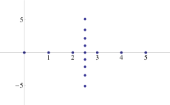
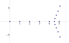
Figure 1: Zeros of $h_{15}^{1,1}(x;5)$ (left) and $h_{15}^{1,15}(x;5)$ (right)

The following result is straightforward taking into account (8) and that if $n\geq N+1$, then $(-N+k)_{n-k}=0$, for $k=0,\dots,N$.

Proposition 3

Let $N$ be a non-negative integer. For every $n\geq N+1$,

$$\begin{array}[]{rl}h_{n}^{\alpha,\beta}(x;N)&=(x-N)_{N+1}(-i)^{n-N-1}p_{n-N-1}(ix;N+1,\beta+N+1,1,\alpha+1)\\ &=(x-N)_{N+1}(-i)^{n-N-1}p_{n-N-1}\left(\left(x-\frac{N}{2}\right)i;1+\frac{N}{2},\beta+1+\frac{N}{2},1+\frac{N}{2},\alpha+1+\frac{N}{2}\right).\end{array}$$

Remark 4

Note that, as was expected from (3), $h_{N+1}^{\alpha,\beta}(x;N)=(x-N)_{N+1}$ which vanishes on $0,1,\dots,N$ and is independent of $\alpha$ and $\beta$ — this fact is non-trivial from the other ways to characterize these polynomials (see e.g. [4]). On the other hand, in the case $\alpha=\beta$ the continuous Hahn polynomial in the right-hand side is a linear transformation of a real polynomial.

Now we establish the main result.

Theorem 5

Let $N$ be a non-negative integer and $\alpha,\beta\in\mathbb{C}$ such that

$$-\alpha,-\beta\not\in\{1,2,\dots,N,N+2,\dots\},$$ (17)

and

$$-\alpha-\beta\not\in\{1,2,\dots,2N+1,2N+3,\dots\}.$$ (18)

Then the family of monic Hahn polynomials $h_{n}^{\alpha,\beta}(x;N)$ for $n\geq 0$ is a MOPS with respect to the following $\Delta$-Sobolev inner product:

$$(f,g)_{S}=\sum_{x=0}^{N}f(x)g(x)\rho^{\alpha,\beta}(x;N)+\int_{C}(\Delta^{N+1}f(z))(\Delta^{N+1}g(z))\omega^{\alpha,\beta}(z;N)dz,$$

where

$$\begin{array}[]{rl}\rho^{\alpha,\beta}(x;N)&=\displaystyle\frac{\Gamma(\beta+N+1-x)\Gamma(\alpha+x+1)}{\Gamma(N+1-x)\Gamma(x+1)},\\ \omega^{\alpha,\beta}(z;N)&=\displaystyle\Gamma(-z)\Gamma(\beta+N+1-z)\Gamma(1+z)\Gamma(\alpha+N+2+z),\end{array}$$

and $C$ is a complex contour from $-\infty i$ to $\infty i$ which separates the poles of the functions $\Gamma(-z)\Gamma(\beta+N+1-z)$ and $\Gamma(1+z)\Gamma(\alpha+N+2+z)$. Furthermore, this $\Delta$-Sobolev inner product characterizes the polynomials $h_{n}^{\alpha,\beta}(x;N)$ for all $n\in\mathbb{N}_{0}$.

Remark 6

Note that the conditions (17) and (18) are equivalent to the existence of a unique $n$ such that $\gamma_{n}=0$, and therefore $n=N+1$. Furthermore, (17) is equivalent to $h_{n}^{\alpha,\beta}(x;N)$ is uniquely determined by (3) for $n\leq N$ together with the poles separation condition of $w^{\alpha,\beta}(z;N)$ given in the above theorem.

[Proof.] If $0\leq m<n\leq N+1$, since $\Delta^{N+1}x^{m}=0$,

$$(h_{n}^{\alpha,\beta}(x;N),x^{m})_{S}=\sum_{x=0}^{N}h_{n}^{\alpha,\beta}(x;N)x^{m}\rho^{\alpha,\beta}(x;N)=0.$$

If $n\geq N+1$ and $m\leq N$, by Proposition 3,

$$(h_{n}^{\alpha,\beta}(x;N),x^{m})_{S}=\sum_{x=0}^{N}h_{n}^{\alpha,\beta}(x;N)x^{m}\rho^{\alpha,\beta}(x;N)=0,$$

and if $N+1\leq m<n$, then

$$\begin{array}[]{rl}(h_{n}^{\alpha,\beta}(x;N),x^{m})_{S}=&\displaystyle\int_{C}(\Delta^{N+1}h_{n}^{\alpha,\beta}(z;N))(\Delta^{N+1}z^{m})\omega^{\alpha,\beta}(z;N)dz\\[8.53581pt] =&\displaystyle\int_{C}p_{n-N-1}(zi;0,\beta+N+1,1,\alpha+N+2)\\ &\times q_{m-N-1}(z)\omega^{\alpha,\beta}(z;N)dz=0,\end{array}$$

where $q_{m-N-1}$ is a polynomial of degree $m-N-1$.

Now we show that the inner product characterizes the polynomials. If $n\leq N$ then, due to (17), we get

$$(h_{n}^{\alpha,\beta}(x;N),x^{n})_{S}=\sum_{x=0}^{N}h_{n}^{\alpha,\beta}(x;N)x^{n}\rho^{\alpha,\beta}(x;N)\neq 0,$$

and if $n\geq N+1$ we obtain

$$\begin{array}[]{rl}(h_{n}^{\alpha,\beta}(x;N),x^{n})_{S}=&\displaystyle\int_{C}(\Delta^{N+1}h_{n}^{\alpha,\beta}(z;N))(\Delta^{N+1}z^{n})\omega^{\alpha,\beta}(z;N)dz\\[8.53581pt] =&\displaystyle\int_{C}p_{n-N-1}(zi;0,\beta+N+1,1,\alpha+N+2)\\ &\times q_{n-N-1}(z)\omega^{\alpha,\beta}(z;N)dz\neq 0,\end{array}$$

since $q_{n-N-1}$ is a polynomial of degree $n-N-1$ and the coefficient $C_{k}$, given in (7), is different from zero for $a=0$, $b=\beta+N+1$, $c=1$, and $d=\alpha+N+2$, for $k=1,2,\dots$ ∎

3 Racah polynomials

We can apply an analogous process for the Racah polynomials

$$R_{n}(\lambda(x);\alpha,\beta,\gamma,\delta)=r_{n}\ {}_{4}F_{3}\left.\left(\begin{array}[]{c}-n,n+\alpha+\beta+1,-x,x+\gamma+\delta+1\\ \alpha+1,\beta+\delta+1,\gamma+1\end{array}\right|1\right),$$ (19)

in which

$$r_{n}=\frac{(\alpha+1,\beta+\delta+1,\gamma+1)_{n}}{(n+\alpha+\beta+1)_{n}},$$

and $\lambda(x)=x(x+\gamma+\delta+1)$, by using the Wilson polynomials [12, p. 28]

$$W_{n}(x^{2};a,b,c,d)=\ w_{n}\ {}_{4}F_{3}\left.\left(\!\!\begin{array}[]{c}-n,n+a+b+c+d-1,a+ix,a-ix\\ a+b,a+c,a+d\end{array}\right|1\right),$$

in which

$$w_{n}=\frac{(-1)^{n}(a+b,a+c,a+d)_{n}}{(n+a+b+c+d-1)_{n}}.$$

In fact,

$$\begin{array}[]{rl}&R_{n}(\lambda(x);\alpha,\beta,\gamma,\delta)\\ &\quad=(-1)^{n}W_{n}\left(\left(ix+i\frac{\gamma+\delta+1}{2}\right)^{2};\frac{\gamma+\delta+1}{2},\alpha-\frac{\gamma+\delta-1}{2},\beta+\frac{-\gamma+\delta+1}{2},\frac{\gamma-\delta+1}{2}\right),\end{array}$$

where $\alpha+1=-N$ or $\beta+\delta+1=-N$ or $\gamma+1=-N$, with $N$ a non-negative integer, and

$$W_{n}(x^{2};a,b,c,d)\!=\!(-1)^{n}R_{n}\left(\lambda(-a\!-\!ix);a+b\!-\!1,c+d\!-\!1,a+d\!-\!1,a\!-\!d\right),$$

where $\lambda(t)=t(t+2a)$.

On the other hand taking, for instance, $\alpha+1=-N$ we get the following factorization for $n>N$:

$$\begin{array}[]{rl}\displaystyle R_{n}(\lambda(x);\alpha,\beta,\gamma,\delta)=&\displaystyle R_{N+1}(\lambda(x);-N-1,\beta,\gamma,\delta)(-1)^{n-N-1}\\ &\times W_{n-N-1}\left(\left(i\bigg{(}x+\frac{\gamma+\delta+1}{2}\bigg{)}\right)^{2};N+\frac{\gamma+\delta+3}{2},\frac{-\gamma-\delta+1}{2},\beta+\frac{-\gamma+\delta+1}{2},\frac{\gamma-\delta+1}{2}\right).\end{array}$$

In this case, the Racah polynomials satisfy the following $\Delta$-Sobolev orthogonality:

$$\langle p,q\rangle_{S}=\langle p,q\rangle_{d}+\left\langle\left(\frac{\Delta}{\Delta\lambda}\right)^{N+1}p,\left(\frac{\Delta}{\Delta\lambda}\right)^{N+1}q\right\rangle_{c},$$

with

$$\begin{array}[]{rl}\langle p,q\rangle_{d}&=\displaystyle\sum_{x=0}^{N}p(x)q(x)\frac{(\alpha+1,\beta+\delta+1,\gamma+1,\gamma+\delta+1,(\gamma+\delta+3)/2)_{x}}{(-\alpha+\gamma+\delta+1,-\beta+\gamma+1,(\gamma+\delta+1)/2,\delta+1,1)_{x}},\\ \langle p,q\rangle_{c}&=\displaystyle\int_{C}p(z^{2})q(z^{2})\nu(zi+i+i\mbox{\small$\frac{{\gamma+\delta+N}}{{2}}$})\nu(-(zi+i+i\mbox{\small$\frac{{\gamma+\delta+N}}{{2}}$}))dz,\end{array}$$

where

$$\nu(z)\equiv\nu(z;a,b,c,d)=\frac{\Gamma(a+iz)\Gamma(b+iz)\Gamma(c+iz)\Gamma(d+iz)}{\Gamma(2z)},$$

being

$$a=1+\frac{\gamma+\delta+N}{2},\ b=\frac{-\gamma-\delta-N}{2},c=\beta+1+\frac{-\gamma+\delta+N}{2},\ d=1+\frac{\gamma-\delta+N}{2},$$

and $C$ is the imaginary axis deformed so as to separate the increasing sequences of poles

$$k,\ \ -1-\gamma-\delta-N+k,\ \ \beta-\gamma+k,\ \ -\delta+k,\qquad k=0,1,2,\dots$$

from the decreasing sequences

$$-\gamma-\delta-N-2-k,\ \ -1-k,\ \ -\beta-\delta-N-2-k,\ \ -\gamma-N-2-k,\qquad k=0,1,2,\dots$$

Of course, we need to assume that these two sets of poles are disjoint, i.e.,

$$2a,\ a+b,\ a+c,\ \dots,\ c+d,\ 2d\not\in\{0,-1,-2,\dots\}.$$

On the other hand, in this case, i.e. $\alpha+1=-N$, we get the following generating functions (see [12, p. 29]) which are valid for all $x\in\mathbb{C}$:

$$\begin{array}[]{rl}\displaystyle\sum_{n=0}^{\infty}\frac{(\alpha+1,\gamma+1)_{n}}{(\alpha-\delta+1)_{n}n!}R_{n}(\lambda(x);\alpha,\beta,\gamma,\delta)t^{n}=&{}_{2}F_{1}\left.\left(\begin{array}[]{c}-x,-x+\beta-\gamma\\ \beta+\delta+1\end{array}\right|t\right)\\ &\displaystyle\times{}_{2}F_{1}\left.\left(\begin{array}[]{c}x+\alpha+1,x+\gamma+1\\ \alpha-\delta+1\end{array}\!\!\right|t\right),\\ \displaystyle\sum_{n=0}^{\infty}\frac{(\alpha+1,\beta+\delta+1)_{n}}{(\alpha-\beta-\gamma+1)_{n}n!}R_{n}(\lambda(x);\alpha,\beta,\gamma,\delta)t^{n}=&\displaystyle{}_{2}F_{1}\left.\left(\begin{array}[]{c}-x,-x-\delta\\ \gamma+1\end{array}\!\!\right|t\right)\\ &\displaystyle\times{}_{2}F_{1}\left.\left(\begin{array}[]{c}x+\alpha+1,x+\beta+\delta+1\\ \alpha+\beta-\gamma+1\end{array}\!\!\right|t\right).\end{array}$$

See e.g. [18] or [11] to get more information about algebraic properties and applications for Wilson polynomials.

4 Dual Hahn polynomials

We can apply an analogous process for the dual Hahn polynomials

$$R_{n}(\lambda(x);\gamma,\delta,N)=(\gamma+1,-N)_{n}\,{}_{3}F_{2}\left.\left(\begin{array}[]{c}-n,-x,x+\gamma+\delta+1\\ \gamma+1,-N\end{array}\right|1\right),$$ (20)

with $\lambda(x)=x(x+\gamma+\delta+1)$, by using the continuous dual Hahn polynomials [12, p. 31]

$$S_{n}(x^{2};a,b,c)=(-1)^{n}(a+b,a+c)_{n}\,{}_{3}F_{2}\left.\left(\begin{array}[]{c}-n,a+ix,a-ix\\ a+b,a+c\end{array}\right|1\right).$$

In fact,

$$\begin{array}[]{rl}&R_{n}(\lambda(x);\gamma,\delta,N)\\ &\quad=(-1)^{n}S_{n}\left(\left(ix+i\frac{\gamma+\delta+1}{2}\right)^{2};\frac{\gamma+\delta+1}{2},\frac{\gamma-\delta+1}{2},-N-\frac{\gamma+\delta+1}{2}\right),\end{array}$$

and

$$S_{n}(x^{2};a,b,c)=(-1)^{n}R_{n}\left(\lambda(-a-ix);a+b-1,a-b,-a-c\right),$$

where $\lambda(t)=t(t+2a)$.

We get the following factorization for $n>N$:

$$\begin{array}[]{rl}\displaystyle R_{n}(\lambda(x);\gamma,\delta,N)=&\displaystyle R_{N+1}(\lambda(x);\gamma,\delta,N)~{}(-1)^{n-N-1}\\ &\times S_{n-N-1}\left(\left(xi+i\frac{\gamma+\delta+1}{2}\right)^{2};N+\frac{\gamma+\delta+2}{2},\frac{-\gamma-\delta+1}{2},\frac{\gamma-\delta+1}{2}\right).\end{array}$$

Dual Hahn polynomials polynomials satisfy the following $\Delta$-Sobolev orthogonality:

$$\langle p,q\rangle_{S}=\langle p,q\rangle_{d}+\left\langle\left(\frac{\Delta}{\Delta\lambda}\right)^{N+1}p,\left(\frac{\Delta}{\Delta\lambda}\right)^{N+1}q\right\rangle_{c},$$

with

$$\begin{array}[]{rl}\langle p,q\rangle_{d}&=\displaystyle\sum_{x=0}^{N}p(x)q(x)\frac{(2x+\gamma+\delta+1)(\gamma+1,-N)_{x}}{(-1)^{x}(x+\gamma+\delta+1)_{N+1}(\delta+1,1)_{x}},\\ \langle p,q\rangle_{c}&=\displaystyle\int_{C}p(z^{2})q(z^{2})w(z;\gamma,\delta,N)dz,\end{array}$$

where

$$w(z;\alpha,\beta,N)=\nu(zi+i+i\mbox{\small$\frac{{\gamma+\delta+N}}{{2}}$};\gamma,\delta,N)\nu(-zi-i-i\mbox{\small$\frac{{\gamma+\delta+N}}{{2}}$};\gamma,\delta,N),$$

being

$$\nu(z;a,b,c)=\frac{\Gamma(a+iz)\Gamma(b+iz)\Gamma(c+iz)}{\Gamma(2zi)},$$

and

$$a=1+\frac{\gamma+\delta+N}{2}\,,\qquad b=1+\frac{\gamma-\delta+N}{2}\,,\qquad c=-\frac{\gamma+\delta+N}{2},$$

and $C$ is the imaginary axis deformed so as to separate the increasing sequences of poles

$$k,\quad-\gamma-\delta-N-1+k,\quad-\delta+k,\qquad k=0,1,2,\dots,$$

from the decreasing sequences

$$-\gamma-\delta-N-2-k,\quad-1-k,\quad-\gamma-N-2-k,\qquad k=0,1,2,\dots$$

Of course, we need to assume that these two sets of poles are disjoint, i.e.,

$$2a,\ a+b,\ a+c,\ \dots,\ 2c\not\in\{0,-1,-2,\dots\}.$$

On the other hand we get the following generating functions (see [12, p. 36]) which are valid for all $x\in\mathbb{C}$:

$$(1-t)^{N-x}{}_{2}F_{1}\left.\left(\begin{array}[]{c}-x,-x-\delta\\ \gamma+1\end{array}\right|t\right)=\sum_{n=0}^{\infty}\frac{(-N)_{n}}{n!}R_{n}(\lambda(x);\gamma,\delta,N)t^{n}.$$

$$(1-t)^{x}{}_{2}F_{1}\left.\left(\begin{array}[]{c}x-N,x+\gamma+1\\ -\delta-N\end{array}\right|t\right)=\sum_{n=0}^{\infty}\frac{(\gamma+1,-N)_{n}}{(-\delta-N)_{n}n!}R_{n}(\lambda(x);\gamma,\delta,N)t^{n}.$$

5 Krawtchouk polynomials

Similarly, properties for the Krawtchouk polynomials

$$K_{n}(x;p,N)=(-N)_{n}p^{n}\,{}_{2}F_{1}\left(\left.\begin{array}[]{cc}-n,-x\\ -N\end{array}\right|\frac{1}{p}\right),$$ (21)

with $p\in\mathbb{C}$, $p\neq 0,1$, can be obtained via Meixner polynomials

$$M_{n}(x;\beta,c)=\frac{c^{n}(\beta)_{n}}{(c-1)^{n}}\,{}_{2}F_{1}\left(\left.\begin{array}[]{c}-n,-x\\ \beta\end{array}\right|1-\frac{1}{c}\right),\quad\beta>0,\ 0<c<1.$$

In fact,

$$\begin{array}[]{rl}K_{n}(x;p,N)&=M_{n}\left(x;-N,\frac{p}{p-1}\right),\\ M_{n}(x;\beta,c)&=K_{n}\left(x;-\beta,\frac{c}{c-1}\right),\end{array}$$

setting $\beta=-N$ and $c=p/(p-1)$.

We have the following factorization for the Krawtchouk polynomials for $n>N$:

$$\begin{array}[]{rl}K_{n}(x;p,N)=&\displaystyle K_{N+1}(x;p,N)M_{n-N-1}(x-N-1;N+2,p/(p-1)).\end{array}$$

Furthermore, these polynomials satisfy the following $\Delta$-Sobolev orthogonality:

$$\langle r,q\rangle_{S}=\langle r,q\rangle_{d}+\left\langle\Delta^{N+1}r,\Delta^{N+1}q\right\rangle_{c},$$

with

$$\langle r,q\rangle_{d} \displaystyle=\sum_{x=0}^{N}r(x)q(x)\frac{p^{x}(1-p)^{N-x}}{\Gamma(x+1)\Gamma(N-x+1)},$$ (22)

$$\langle r,q\rangle_{c} =\displaystyle\int_{C}r(z)q(z)\Gamma(-z)\Gamma(1+z)\left(\frac{p}{1-p}\right)^{z}dz,$$ (23)

where $C$ is the imaginary axis deformed so as to separate the increasing from the decreasing sequence of poles of the weight function, in fact in this case we can consider the curve $C=\{-1/2+ti:t\in\mathbb{R}\}$.

Remark 7

Note that the property of orthogonality for the Krawtchouk polynomials (22) is valid for all $p\in\mathbb{C}$, with $p\neq 0,1$ by using an analytic continuation for the standard weight function associated with the Krawtchouk polynomials.

On the other hand, we get the following generating function (see [12, p. 47]) which is valid for all $x\in\mathbb{C}$:

$$\left(1-\frac{1-p}{p}~{}t\right)^{x}(1+t)^{N-x}=\sum_{n=0}^{\infty}{N\choose n}K_{n}(x;p,N)t^{n}.$$

6 Limit relations between hypergeometric orthogonal polynomials

In this section, we study the limit relations involving the orthogonal polynomials, considered in this paper, associated with some families of polynomials of the Askey scheme of hypergeometric orthogonal polynomials [12].

Let us now consider such limits for any $n\in\mathbb{N}_{0}$:

1. Racah $\to$ Hahn. If we take $\gamma+1=-N$ and $\delta\to\infty$ in the definition (19) of the Racah polynomials, we obtain the Hahn polynomials defined by (2). Hence

   $$\lim_{\delta\to\infty}R_{n}(\lambda(x);\alpha,\beta,-N-1,\delta)=h_{n}^{\alpha,\beta}(x;N).$$

   The Hahn polynomials can also be obtained from the Racah polynomials by taking $\delta=-\beta-N-1$ in the definition (19) and letting $\gamma\to\infty$:

   $$\lim_{\gamma\to\infty}R_{n}(\lambda(x);\alpha,\beta,\gamma,-\beta-N-1))=h_{n}^{\alpha,\beta}(x;N).$$

   Another way to do this is to take $\alpha+1=-N$ and $\beta\to\beta+\gamma+N+1$ in the definition (19) of the Racah polynomials and then take the limit $\delta\to\infty$. In that case we obtain the Hahn polynomials given by (2) in the following way:

   $$\lim_{\delta\to\infty}R_{n}(\lambda(x);-N-1,\beta+\gamma+N+1,\gamma,\delta)=h_{n}^{\gamma,\beta}(x;N).$$

2. Racah $\to$ Dual Hahn. If we take $\alpha+1=-N$ and let $\beta\to\infty$ in the definition (19) of the Racah polynomials, then we obtain the dual Hahn polynomials defined by (20). Hence

   $$\lim_{\beta\to\infty}R_{n}(\lambda(x);-N-1,\beta,\gamma,\delta)=R_{n}(\lambda(x);\gamma,\delta,N).$$

   If we take $\beta=-\delta-N-1$ and $\alpha\to\infty$ in (19), then we also obtain the dual Hahn polynomials:

   $$\lim_{\alpha\to\infty}R_{n}(\lambda(x);\alpha,-\delta-N-1,\gamma,\delta)=R_{n}(\lambda(x);\gamma,\delta,N).$$

   Finally, if we take $\gamma+1=-N$ and $\delta\to\alpha+\delta+N+1$ in the definition (19) of the Racah polynomials and take the limit $\beta\to\infty$ we find the dual Hahn polynomials given by (20) in the following way:

   $$\lim_{\beta\to\infty}R_{n}(\lambda(x);\alpha,\beta,-N-1,\alpha+\delta+N+1)=R_{n}(\lambda(x);\alpha,\delta,N).$$

3. Hahn $\to$ Krawtchouk. If we take $\alpha=(1-p)t$ and $\beta=pt$ in the definition (2) of the Hahn polynomials and let $t\to\infty$ we obtain the Krawtchouk polynomials defined by (21):

   $$\lim_{t\to\infty}h_{n}^{(1-p)t,pt}(x;N)=K_{n}(x;p,N).$$

4. Dual Hahn $\to$ Krawtchouk. In the same way we find the Krawtchouk polynomials from the dual Hahn polynomials by setting $\gamma=pt$, $\delta=(1-p)t$ in (20) and letting $t\to\infty$:

   $$\lim_{t\to\infty}R_{n}(\lambda(x);pt,(1-p)t,N)=K_{n}(x;p,N).$$

Remark 8

The proof of each one of these limits is straightforward once one reduces the hypergeometric representation of each family as we did for the Hahn polynomials (see (8)) which is valid for all $n\in\mathbb{N}_{0}$.

Appendix A Orthogonality relations for Meixner polynomials with general parameter

In this appendix we will show that Meixner polynomials, $\{M_{n}(x;\beta,c)\}_{n\geq 0}$, with $c<0$ and $\beta\in\mathbb{C}$, can be provided with a property of orthogonality which can be obtained through a process limit from the continuous Hahn polynomials.

From the TTRR of the continuous Hahn polynomials it is straightforward to obtain the following relation

$$p_{n+1}(ix;0,-\mbox{\small$\frac{{t}}{{c}}$},t,\beta)=(x\!-\!B_{n})p_{n}(ix;0,-\mbox{\small$\frac{{t}}{{c}}$},t,\beta)\!-\!C_{n}p_{n-1}(ix;0,-\mbox{\small$\frac{{t}}{{c}}$},t,\beta),$$ (24)

where $t\in\mathbb{R}^{+}$, and

$$\begin{array}[]{rl}B_{n}&=\frac{n\left(n-\frac{t}{c}+t-1\right)\left(n-\frac{t}{c}+\beta-1\right)}{\left(2n-\frac{t}{c}+t+\beta-2\right)\left(2n-\frac{t}{c}+t+\beta-1\right)}-\frac{\left(n-\frac{t}{c}+t+\beta-1\right)(n+t)(n+\beta)}{\left(2n-\frac{t}{c}+t+\beta-1\right)\left(2n-\frac{t}{c}+t+\beta\right)},\\ C_{n}&=\frac{n\left(n-\frac{t}{c}+t-1\right)\left(n-\frac{t}{c}+\beta-1\right)\left(n-\frac{t}{c}+t+\beta-2\right)(n+t-1)(n+\beta-1)}{\left(2n-\frac{t}{c}+t+\beta-1\right)\left(2n-\frac{t}{c}+t+\beta-2\right)^{2}\left(2n-\frac{t}{c}+t+\beta-3\right)}.\end{array}$$

Since

$$\begin{array}[]{rl}\lim_{|t|\to\infty}B_{n}&=\displaystyle\frac{n+c(n+\beta)}{1-c},\\ \lim_{|t|\to\infty}-C_{n}&=\displaystyle\frac{nc(n+\beta-1)}{(c-1)^{2}},\end{array}$$

coincide with the coefficients of the TTRR for the monic Meixner polynomials, with initial conditions $p_{-1}=0$ and $p_{0}=1$, one deduces

$$\lim_{|t|\to\infty}(-i)^{n}p_{n}(ix;0,-t/c,t,\beta)=M_{n}(x;\beta,c),\qquad n=0,1,2,\dots,$$ (25)

by using induction in (24).

Proposition 9

For any $\beta,c\in\mathbb{C}$, $c\notin[0,\infty)$ and $-\beta\not\in\mathbb{N}$, the following property of orthogonality for the Meixner polynomials fulfills:

$$\int_{C}\!\!M_{n}(z;c,\beta)z^{m}\Gamma(-z)\Gamma(\beta+z)(-c)^{z}dz=0,\ 0\leq m<n,\ n=0,1,2,\dots$$ (26)

where $C$ is a complex contour from $-\infty i$ to $\infty i$ separating the increasing poles $\{0,1,2,\dots\}$ from the decreasing poles $\{-\beta,-\beta-1,-\beta-2,\dots\}$.

[Proof.] We prove the result for $c<0$, thus the general case is obtained by analytic continuation.

Let us assume that $\beta$ is such that the contour $C=\{-1/2+yi:y\in\mathbb{R}\}$ separates the poles of $\Gamma(\beta+z)$ from the poles of $\Gamma(-z)$, i.e., $\Re\beta>1/2$, and let us take the normalized weight for the continuous Hahn polynomials (see (6))

$$W_{t}(z)=\frac{w(iz;0,-t/c,t,\beta)}{\Gamma(-t/c)\Gamma(t)}=\Gamma(-z)~{}\frac{\Gamma(-t/c-z)}{\Gamma(-t/c)}~{}\frac{\Gamma(t+z)}{\Gamma(t)}~{}\Gamma(\beta+z).$$

Notice that

$$\lim_{t\to\infty}W_{t}(z)=\Gamma(-z)\Gamma(\beta+z)(-c)^{z}=:W(z),$$

pointwise in $C$ by using the Stirling formula

$$\Gamma(z)=\sqrt{2\pi}z^{z-{\textstyle\frac{1}{2}}}e^{-z}(1+o(1)),\qquad z\to\infty,|\arg(z)|<\pi.$$

It is known that

$$|\Gamma(x+iy)|\leq|\Gamma(x)|,\qquad\forall\,x,y\in\mathbb{R},$$

hence

$$|W_{t}(z)|\leq\left|\Gamma(-z)~{}\Gamma(\beta+z)\right|\,.$$ (27)

Using once again induction on (24) and due to the exponential behavior of the right-hand side of (27) at the endpoints of $C$, one obtains that

$$p_{n}(iz;0,-t/c,t,\beta)W_{t}(z)$$

is dominated by an integrable function on $C$. Thus, from the dominated convergence theorem

$$\lim_{t\to\infty}\int_{C}(-i)^{n+1}p_{n}(iz;0,-t/c,t,\beta)z^{m}W_{t}(z)dz=\int_{C}M_{n}(z;\beta,c)z^{m}W(z)dz.$$

On the other side since $C$ also separates the poles of $\Gamma(-t/c-z)$ from the poles of $\Gamma(t+z)$, we get

$$\int_{C}(-i)^{n+1}p_{n+1}(iz;0,-t/c,t,\beta)z^{m}W_{t}(z)=0.$$

Thus (26) holds for $\Re\beta>1/2$.

The general case is straightforward by using that if $C$ is a contour separating the poles and $C_{1}=\{\lambda+yi:y\in\mathbb{R}\}$, where $\lambda\in(0,1)$, $\lambda\neq\Re\beta$, which does not separate the poles, then the integral through $C$ and $C_{1}$ differs on a finite number of residues. ∎

The case $c>0$ cannot be considered by an integral of the form (26) since it diverges. However, when $|c|<1$, (26) is rewritten on the form (see [17, §5.6] for details)

$$\sum_{x=0}^{\infty}M_{n}(x;c,\beta)x^{m}~{}\frac{\Gamma(\beta+x)~{}c^{x}}{x!}=0,$$

which is also valid for $c\in(0,1)$ and coincides with the very well-known orthogonal relations for Meixner polynomials.

Acknowledgements: We thank referees for their suggestions which have improved the presentation of the paper.
The authors also wish to thank R. Álvarez-Nodarse, F. Marcellán, J.J. Moreno-Balcázar and A. Zarzo, for their useful suggestions and comments.

References

• [1] M. Alfaro and R. Álvarez-Nodarse. A characterization of the classical orthogonal discrete and $q$-polynomials. J. Comput. Appl. Math. 201 (2007) 48–54.
• [2] M. Alfaro, T. E. Pérez, M. A. Piñar, and M. L. Rezola. Sobolev orthogonal polynomials: the discrete-continuous case. Methods Appl. Anal. 6 (1999) 593–616.
• [3] M. Alfaro, M. Álvarez de Morales, and M. L. Rezola. Orthogonality of the Jacobi polynomials with negative integer parameters. J. Comput. Appl. Math. 145 (2002) 379–386.
• [4] R. Álvarez-Nodarse. On characterizations of classical polynomials. J. Comput. Appl. Math. 196 (2006) 320-337.
• [5] R. Askey. Continuous Hahn polynomials. J. Phys A: Math. Gen. 18 (1985) 1017–1019.
• [6] N. M. Atakishiev and S. K. Suslov. The Hahn and Meixner polynomials of an imaginary argument and some of their applications. J. Phys A: Math. Gen. 18 (1985) 1583–1596.
• [7] M. Álvarez de Morales, T. E. Pérez, and M. A. Piñar. Sobolev orthogonality for the Gegenbauer polynomials $\{C_{n}^{(-N+1/2)}\}_{n\geq 0}$. J. Comput. Appl. Math. 100 (1998) 111–120.
• [8] M. Álvarez de Morales, T. E. Pérez, M. A. Piñar, and A. Ronveaux. Non-standard orthogonality for Meixner polynomials. Electron. Trans. Numer. Anal. 9 (1999) 1–25.
• [9] K. H. Kwon and L. L. Littlejohn. The orthogonality of the Laguerre polynomials $\{L_{n}^{(-k)}(x)\}$ for a positive integer $k$. Ann. Numer. Math. 2 (1995) 289–304.
• [10] K. H. Kwon and L. L. Littlejohn. Sobolev orthogonal polynomials and second-order differential equations. Rocky Mountain J.Math. 28(2) (1998) 547–594.
• [11] S. Karlin and J. McGregor. The Hahn polynomials, formulas and applications. Scripta Math. 26 (1961) 33–46.
• [12] R. Koekoek and R. F. Swarttouw. The Askey-scheme of hypergeometric orthogonal polynomials and its $q$-analogue, volume 98-17. Reports of the Faculty of Technical Mathematics and Informatics, Delft, The Netherlands, 1998.
• [13] A. F. Nikiforov, S. K. Suslov, and V. B. Uvarov Classical orthogonal polynomials of a discrete variable. Springer Series in Computational Physics, Springer-Verlag, NewYork, 1991.
• [14] T. E. Pérez and M. A. Piñar. On Sobolev orthogonality for the generalized Laguerre polynomials. J. Approx. Theory 86 (1996) 278–285.
• [15] T. E. Pérez and M. A. Piñar. Sobolev orthogonality and properties of the generalized Laguerre polynomials. In William B. Jones and A. Sri Ranga, editors, Orthogonal Functions, Moment Theory and Continued Fractions: Theory and Applications, volume 18, New York, 1997, pp.375–385.
• [16] F. Marcellán and J. J. Moreno–Balcázar. Asymptotics and zeros of Sobolev orthogonal polynomials on unbounded supports. Acta Appl. Math. 94 (2006) 163–192.
• [17] N. M. Temme. Special functions. An introduction to the classical functions of Mathematical Physics. John Wiley and Sons, New York, 1996.
• [18] J. A. Wilson. Some hypergeometric orthogonal polynomials. SIAM J. Math. Anal. 11 (1980) 690–701.