Breakdown of the Fermi-liquid regime in the 2D Hubbard model from a two-loop field-theoretical renormalization group approach

Abstract

We analyze the particle-hole symmetric two-dimensional Hubbard model on a square lattice starting from weak-to-moderate couplings by means of the field-theoretical renormalization group (RG) approach up to two-loop order. This method is essential in order to evaluate the effect of the momentum-resolved anomalous dimension $\eta(\textbf{p})$ which arises in the normal phase of this model on the corresponding low-energy single-particle excitations. As a result, we find important indications pointing to the existence of a non-Fermi liquid (NFL) regime at temperature $T\rightarrow 0$ displaying a truncated Fermi surface (FS) for a doping range exactly in between the well-known antiferromagnetic insulating and the $d_{x^{2}-y^{2}}$-wave singlet superconducting phases. This NFL evolves as a function of doping into a correlated metal with a large FS before the $d_{x^{2}-y^{2}}$-wave pairing susceptibility finally produces the dominant instability in the low-energy limit.

I Introduction

The physical nature of underdoped cuprates both above and below the superconducting temperature $T_{c}$ is still subjected to strong debate Millis ; Timusk ; Norman . The recent experiment of Doiron-Leyraud et al. Leyraud applying a magnetic field strong enough to destroy the superconducting state established the existence of quantum oscillations and coherent Fermi surface (FS) pockets for this regime. By contrast, earlier angle-resolved photoemission experiments (ARPES) reported only observations of disconnected Fermi arcs located in the nodal regions of momentum space Ding ; Loeser . Moreover, according to both scenarios, there exist charge pseudogaps and no quasiparticle-like excitations in the corresponding antinodal sectors centered around $(\pm\pi,0)$ and $(0,\pm\pi)$. The absence of these quasiparticle excitations is signalled by the vanishing of the quasiparticle peak $Z(\mathbf{p})$ in the spectral function at these antinodal regions. The pseudogap behavior also reflects itself in the underdoped superconducting phase. One manifestation of this is the fact that the superconducting gap and the pseudogap behave distinctively as a function of doping: the superconducting gap located in the nodal regions centered around $(\pm\pi/2,\pm\pi/2)$ decreases continuously whereas the pseudogap continues to increase as the hole doping is reduced from its optimal value Shen ; Tanaka . Such a nodal-antinodal dichotomy is therefore a common trend in underdoped cuprates.

A minimal model for describing the dynamics of the interacting electrons in these high-$T_{c}$ superconductors is the single-band 2D Hubbard model Anderson . This model has been investigated extensively with several numerical techniques such as exact diagonalization, quantum Monte Carlo and the more recent quantum clusters approaches Maier ; Kyung , as well as by semi-analytical functional renormalization group (RG) methods Zanchi ; Metzner ; Honerkamp ; Shankar ; Kopietz ; Tsai ; Gonzalez ; Binz ; Ferraz . Several of these works successfully obtain an antiferromagnetic phase in the model near half-filling and the onset of a $d_{x^{2}-y^{2}}$-wave singlet superconducting phase away from half-filling when the temperature is lowered below a critical value Zanchi ; Metzner ; Honerkamp ; Maier . These results therefore give further support to the point of view that the 2D Hubbard model might indeed capture the essential aspects of the physics displayed by those strongly-correlated materials.

On the experimental side, the insulating antiferromagnetic phase in the hole-doped cuprates is quickly destroyed at a very small but nevertheless nonzero doping. If we approach this phase from a larger doping regime, this suggests that the existing Fermi surface should shrink to zero with the corresponding quasiparticle weight $Z(\mathbf{p})$ becoming suppressed all along the underlying FS at a possible quantum critical point. It is therefore clearly important to account for the physical effects associated with such a vanishing of $Z$ at a nonzero doping near half-filling. This analysis has been initiated in recent years for the 2D Hubbard model and its extensions in the context of the fermionic RG framework Zanchi2 ; Honerkamp2 ; Katanin ; Metzner2 . However, since the self-energy effects manifest themselves only at two-loop order or beyond, in order to devise conserving many-body approximations comment for this model, one should necessarily evaluate all flow equations up to the same order of perturbation theory. For this reason, we implement in this work a two-loop field-theoretical RG calculation as a function of doping concentration for some important quantities in the 2D Hubbard model.

Following previous one-loop RG calculations performed in the 2D Hubbard model, we choose to consider here only weak-to-moderate initial couplings. As a result, we find important indications pointing to the existence of a non-Fermi liquid (NFL) regime at a nonzero doping, before the $d_{x^{2}-y^{2}}$-wave singlet superconducting instability finally dominates over the antiferromagnetic fluctuations. An important point we wish to stress here is that this NFL regime emerges from the nonzero momentum-resolved anomalous dimension $\eta(\mathbf{p})$ contribution to the single-particle excitations, which arises only at a two-loop RG level or beyond close to half-filling. In the corresponding one-loop RG flow equations, even if the initial values are taken to be reasonably small, the renormalized interactions rapidly flow towards a strong coupling regime in the low-energy limit. This fact also indicates the importance of higher-order quantum corrections to the full description of the low-energy dynamics of the 2D Hubbard model. Our work therefore takes seriously this observation and, for this reason, it represents a step forward in this direction.

This paper is organized as follows. In Sec. II, we explain the methodology employed to discuss the 2D Hubbard model. In this part, we will choose to be very schematic since the fermionic field-theoretical RG methodology was already explained at length and in full detail in the context of a simpler 2D flat FS model elsewhere Hermann . Our main emphasis will be rather to highlight the final integro-differential two-loop RG flow equations resulting from the application of this method to the 2D Hubbard model. In Sec. III, we move on to the numerical solution of these RG flow equations. Lastly, in Sec. IV, we present our final conclusions regarding our two-loop RG calculation and we point out open issues that still have to addressed for the full clarification of this important problem.

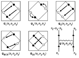
Figure 1: The g-ology parametrization for the marginally relevant interaction processes of the 2D Hubbard model, using as a reference the corresponding noninteracting FS at half-filling for simplicity.

II Methodology

We start by defining the Hamiltonian of the 2D Hubbard model in momentum space

$$H=\sum_{\mathbf{k},\sigma}\xi_{\mathbf{k}}\psi^{\dagger}_{\mathbf{k}\sigma}\psi_{\mathbf{k}\sigma}+\left(\frac{U}{N_{s}}\right)\sum_{\mathbf{p},\mathbf{k},\mathbf{q}}\psi^{\dagger}_{\mathbf{p}+\mathbf{k}-\mathbf{q}\uparrow}\psi^{\dagger}_{\mathbf{q}\downarrow}\psi_{\mathbf{k}\downarrow}\psi_{\mathbf{p}\uparrow}.$$ (1)

where $\psi^{\dagger}_{\mathbf{k}\sigma}$ and $\psi_{\mathbf{k}\sigma}$ are the usual fermionic creation and annihilation operators with momentum $\mathbf{k}$ and spin projection $\sigma$, $t$ is the electronic hopping amplitude to nearest neighbor sites, $\mu$ is the chemical potential which controls the band filling (and, consequently, the doping parameter), $U$ is the local on-site repulsive interaction and $N_{s}$ is the total number of lattice sites. Since we will be interested only in the universal quantities of this model, we can linearize the tight-binding energy dispersion $\xi_{\mathbf{k}}=-2t\big{[}\cos(k_{x})+\cos(k_{y})\big{]}-\mu$ around the FS as $\xi_{\mathbf{k}}\approx v_{F}(\mathbf{k})\mathbf{\hat{n}}.\big{(}\mathbf{k-k_{F}}(\mu)\big{)}$ with the Fermi velocity given by $v_{F}(\mathbf{k})=\big{|}(\nabla_{\mathbf{k}}\xi_{\mathbf{k}}\small|_{\mathbf{k=k_{F}}(\mu)})\big{|}=2t\sqrt{\sin^{2}k_{x}+\sin^{2}k_{y}}$, $\mathbf{k_{F}}(\mu)$ being the Fermi momentum which defines the noninteracting FS for a continuous doping parameter and $\mathbf{\hat{n}}$ is a unit vector perpendicular to the FS.

The thermodynamical properties of this model can be computed from the coherent-state Grassmann representation of the partition function

$$Z=\int\mathcal{D}[\bar{\psi},\psi]e^{-\int_{0}^{\beta}d\tau(L_{0}[\bar{\psi},\psi]+L_{int}[\bar{\psi},\psi])},$$ (2)

where $\beta=1/T$. The noninteracting Lagrangian is defined in a standard way

$$L_{0}[\bar{\psi},\psi]=\sum_{\sigma}\int_{\mathbf{k}}\bar{\psi}_{\sigma}(\mathbf{k},\tau)\big{(}\partial_{\tau}+\xi_{\mathbf{k}}\big{)}\psi_{\sigma}(\mathbf{k},\tau),$$ (3)

where $\int_{\mathbf{k}}=\int\frac{d^{2}\mathbf{k}}{(2\pi)^{2}}$ and the interacting Lagrangian in turn reads

$$L_{int}[\bar{\psi},\psi]=\sum_{\sigma,\sigma^{\prime}}\int_{\mathbf{p_{1}}}\int_{\mathbf{p_{2}}}\int_{\mathbf{p_{3}}}g(\mathbf{p_{1},p_{2},p_{3}})$$

$$\times\bar{\psi}_{\sigma}(\mathbf{p_{1}+p_{2}-p_{3}},\tau)\bar{\psi}_{\sigma^{\prime}}(\mathbf{p_{3}},\tau)\psi_{\sigma^{\prime}}(\mathbf{p_{2}},\tau)\psi_{\sigma}(\mathbf{p_{1}},\tau).$$

(4)

The Eqs. (3) and (4) therefore define our bare quantum field theory which is regularized in the ultraviolet by restricting the momenta to $|\mathbf{k}|\leq\Lambda_{0}$, where the cutoff is chosen to be $\Lambda_{0}=4t$. Since this should correspond originally to the 2D Hubbard model, we must set the bare interaction $g(\mathbf{p_{1},p_{2},p_{3}})$ initially equal to the local interaction $U$. However, as we will see next, this functional dependence of the coupling on the momenta will in fact play a crucial role in the low-energy effective theory.

Here we perform all the calculations in the $T\rightarrow 0$ limit. The starting point of our approach is the noninteracting FS of the 2D Hubbard model defined by $\mathbf{k_{F}}(\mu)$ for a continuous doping parameter. To include the effect of interactions, we use a g-ology parametrization adapted appropriately to our 2D problem (for more details on this procedure in the context of a simpler 2D flat FS model, see, e.g., Ref. Hermann ). By means of a power counting analysis, one can easily verify that the dependence of the coupling function $g(\mathbf{p_{1},p_{2},p_{3}})$ on the components of the momenta normal to the FS are irrelevant in the RG sense. Therefore, we are allowed to project these coupling functions on the FS in such a way that their only functional dependence will come from the components parallel to the FS of the three external momenta $\mathbf{p_{1}}$, $\mathbf{p_{2}}$, and $\mathbf{p_{3}}$ (the fourth momentum is given naturally by momentum conservation $\mathbf{p_{4}}=\mathbf{p_{1}}+\mathbf{p_{2}}-\mathbf{p_{3}}$). In this way, we consider here the interaction processes which lead to singularities within perturbation theory in the low-energy limit. They are shown schematically in Fig. 1. These processes are the marginally relevant couplings in our RG theory, since their contributions become increasingly important at low energies. We neglect here the so-called $g_{4}$-processes of interacting particles belonging to the same FS sector. Experience with one-dimensional systems suggests that they should not alter qualitatively our results. Besides, we also neglect all marginally irrelevant interactions, since these contributions are not expected to change the universal properties of the model.

The methodology of our RG scheme follows closely the field-theoretical method Peskin ; Weinberg . In perturbation theory, infrared logarithmic singularities typically emerge in the low-energy limit at the calculation of several quantities in the model such as the vertex corrections, the quasiparticle weight and the susceptibilities. We circumvent this problem by introducing appropriate counterterms at a flowing RG scale parameter $\Lambda$, in such a way that all the observables – i.e. the renormalized quantities of the theory – remain well-defined in the low-energy limit ($\Lambda\rightarrow 0$). As we have already pointed out in an earlier paper Hermann , the problem of formulating a RG theory associated with a FS of a 2D model often requires the definition of counterterms which are continuous functions of the parallel momenta along the FS. In this way, we must perform at two-loop level the following substitutions for the fermionic fields

$$\psi_{\sigma}(\mathbf{p},\tau)\rightarrow Z_{\Lambda}^{1/2}(\mathbf{p})\psi_{\sigma}(\mathbf{p},\tau),$$

$$\bar{\psi}_{\sigma}(\mathbf{p},\tau)\rightarrow Z_{\Lambda}^{1/2}(\mathbf{p})\bar{\psi}_{\sigma}(\mathbf{p},\tau),$$ (5)

where, from now on, all the momenta will correspond to the momentum projected on the FS. Besides, $Z_{\Lambda}(\mathbf{p})$ is the RG flowing momentum-resolved quasiparticle weight and it is naturally related in the limit of $\Lambda\rightarrow 0$ to the conventional many-body definition of the quasiparticle peak $Z(\mathbf{p})=(1-\partial\rm Re\Sigma(\omega,\mathbf{p})/\partial\omega|_{\omega=0})^{-1}$. Using Eq. (5), we also find that the bare and renormalized coupling functions are related to each order by

$$g_{i}(\mathbf{p_{1}},\mathbf{p_{2}},\mathbf{p_{3}})=\left[\prod_{j=1}^{4}Z_{\Lambda}^{-1/2}(\mathbf{p_{j}})\right]\bigg{(}g_{iR}(\mathbf{p_{1}},\mathbf{p_{2}},\mathbf{p_{3}};\Lambda)$$

$$+\Delta g_{iR}^{1loop}(\mathbf{p_{1}},\mathbf{p_{2}},\mathbf{p_{3}};\Lambda)+\Delta g_{iR}^{2loops}(\mathbf{p_{1}},\mathbf{p_{2}},\mathbf{p_{3}};\Lambda)\bigg{)},$$

(6)

where $i=$1, 2, 3, 3X, and BCS. The renormalized quantities (labeled by the subscript $R$) generally depend on the RG scale $\Lambda$. In contrast, all the bare quantities will be denoted here without any additional index. The functions $\Delta g_{iR}^{1loop}(\mathbf{p_{1}},\mathbf{p_{2}},\mathbf{p_{3}};\Lambda)$ and $\Delta g_{iR}^{2loops}(\mathbf{p_{1}},\mathbf{p_{2}},\mathbf{p_{3}};\Lambda)$ represent the counterterms necessary to regularize at one-loop and two-loops respectively the four-point one-particle irreducible (1PI) vertex corrections in each of the corresponding parametrized scattering channels.

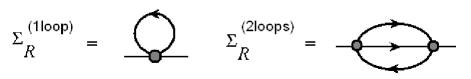
Figure 2: The self-energy diagrams up to two-loop order. The one-loop term is the Hartree diagram and the two-loop contribution is the so-called sunset diagram.

Following the same strategy as it was described in full detail in Ref. Hermann , we now calculate the quasiparticle weight $Z_{\Lambda}(\mathbf{p})$ at two-loop level starting from the definition of the renormalized self-energy of the present model. The corresponding Feynman diagrams up to two-loop order are shown in Fig. 2. The one-loop diagram (i.e., the Hartree term) is generally independent of the external frequency $\omega$. As a result, this contribution never renormalizes the quasiparticle weight. In fact, it only generates a constant shift in the chemical potential of the model which must be appropriately subtracted by a counterterm in such a way that the density of particles in the system always remains fixed during the RG flow. By contrast, the two-loop contribution (i.e., the sunset diagram) is the first contribution to the self-energy which produces a nonanalyticity as a function of the external frequency $\omega$. For this reason, this term alone will be responsible for the renormalization of the quasiparticle weight $Z_{\Lambda}(\mathbf{p})$ at this level of perturbation theory as we vary the RG scale $\Lambda$ towards the low-energy limit.

The momentum-resolved anomalous dimension is conventionally defined by $\eta(\mathbf{p})=\Lambda d\ln Z_{\Lambda}(\mathbf{p})/d\Lambda$. From this expression, we get

$$\eta(\mathbf{p}) = \frac{1}{8\pi^{4}}\int_{FS}d\mathbf{k}\int_{FS}d\mathbf{q}\left[\frac{\Lambda}{\Lambda+2|\mu|F(\mathbf{p},\mathbf{k},\mathbf{q})}\right]$$

$$\times \big{[}2g_{1R}(\mathbf{p},\mathbf{k+q-p},\mathbf{k})g_{1R}(\mathbf{k},\mathbf{q},\mathbf{p})$$

$$+ 2g_{2R}(\mathbf{p},\mathbf{k}\mathbf{+q-p},\mathbf{q})g_{2R}(\mathbf{k},\mathbf{q},\mathbf{k+q-p})$$

$$- g_{1R}(\mathbf{p},\mathbf{k+q-p},\mathbf{k})g_{2R}(\mathbf{k},\mathbf{q},\mathbf{k+q-p})$$

$$- g_{2R}(\mathbf{p},\mathbf{k+q-p},\mathbf{q})g_{1R}(\mathbf{k},\mathbf{q},\mathbf{p})+2g_{3R}(\mathbf{k},\mathbf{p},\mathbf{q})$$

$$\times g_{3R}(\mathbf{k},\mathbf{p},\mathbf{q})-g_{3R}(\mathbf{k},\mathbf{p},\mathbf{q})g_{3R}(\mathbf{p},\mathbf{k},\mathbf{q})\big{]}$$

$$\times \left(\frac{1}{v_{F}(\mathbf{k})+v_{F}(\mathbf{q})}\right)\left(\frac{1}{v_{F}(\mathbf{q})+v_{F}(\mathbf{k+q-p})}\right),$$

where the integrals over the momenta now are simply along the curve defined by the FS and, besides, $F(\mathbf{p},\mathbf{k},\mathbf{q})=v_{F}(\mathbf{k+q-p})/v_{F}(\mathbf{k})$. It is interesting to note here that if we take the 1D limit of the above equation, we reproduce exactly the well-known result for the anomalous dimension of the Luttinger liquid at two-loop order as was first calculated long ago in Ref. Solyom .

To derive the two-loop RG flow equations for the renormalized coupling functions, we must take into account the fact that the bare theory does not know anything about the RG scale $\Lambda$. In other words, the bare couplings do not depend on this scale, i.e. $\Lambda dg_{i}(\mathbf{p_{1}},\mathbf{p_{2}},\mathbf{p_{3}})/d\Lambda=0$. Therefore, using Eq. (6), we finally obtain

$$\Lambda\frac{d}{d\Lambda}g_{iR}(\mathbf{p_{1}},\mathbf{p_{2}},\mathbf{p_{3}})=\frac{1}{2}\sum_{i=1}^{4}\eta(\mathbf{p_{i}})g_{iR}(\mathbf{p_{1}},\mathbf{p_{2}},\mathbf{p_{3}})$$

$$-\Lambda\frac{d}{d\Lambda}\Delta g_{iR}^{1loop}(\mathbf{p_{1}},\mathbf{p_{2}},\mathbf{p_{3}})-\Lambda\frac{d}{d\Lambda}\Delta g_{iR}^{2loops}(\mathbf{p_{1}},\mathbf{p_{2}},\mathbf{p_{3}}),$$

(8)

where $i=$1, 2, 3, 3X, and BCS. The Feynman diagrams for the vertex corrections necessary for the determination of the counterterm functions are shown schematically in Fig. 3. These RG flow equations for the renormalized couplings are in fact complicated integro-differential equations coupled to one another. We will discuss their numerical solution in the next section.

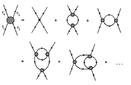
Figure 3: Some Feynman diagrams showing the vertex corrections up to two-loop order.

To investigate what are the enhanced correlations in low-energy limit of the 2D Hubbard model, we must calculate the linear response of the system to small external fields. Therefore, we must add to our original Lagrangian the folllowing term

$$L_{ext} = \int_{\mathbf{q,p}}\bigg{[}h_{SC}(\mathbf{q})\gamma^{\alpha\beta}_{SC}(\mathbf{p,q})\bar{\psi}_{\alpha}(\mathbf{p},\tau)\bar{\psi}_{\beta}(\mathbf{-p+q},\tau)$$

$$+ h_{DW}(\mathbf{q})\gamma^{\alpha\beta}_{DW}(\mathbf{p,q})\bar{\psi}_{\alpha}(\mathbf{p+q},\tau)\psi_{\beta}(\mathbf{p},\tau)+h.c.\bigg{]}$$

where $h_{SC}(\mathbf{q})$ and $h_{DW}(\mathbf{q})$ are the external fields and $\gamma^{\alpha\beta}_{SC}(\mathbf{p,q})$ and $\gamma^{\alpha\beta}_{DW}(\mathbf{p,q})$ are the response vertices for superconducting and density-wave orders respectively Eberth . This added term will generate new Feynman diagrams – the three-legged vertices displayed in Fig. 4 – which will also generate new logarithmic singularities in the low-energy limit of our quantum field theory. Therefore, we must regularize these divergences by defining new counterterms as follows

$$\gamma^{\alpha\beta}_{SC}(\mathbf{p,q}) = Z_{\Lambda}^{-1/2}(\mathbf{p})Z_{\Lambda}^{-1/2}(\mathbf{-p+q})\bigg{[}\gamma^{\alpha\beta}_{R,SC}(\mathbf{p,q};\Lambda)$$

$$+ \Delta\gamma^{\alpha\beta}_{R,SC}(\mathbf{p,q};\Lambda)\bigg{]}$$

$$\gamma^{\alpha\beta}_{DW}(\mathbf{p,q}) = Z_{\Lambda}^{-1/2}(\mathbf{p+q})Z_{\Lambda}^{-1/2}(\mathbf{p})\bigg{[}\gamma^{\alpha\beta}_{R,DW}(\mathbf{p,q};\Lambda)$$ (10)

$$+ \Delta\gamma^{\alpha\beta}_{DW}(\mathbf{p,q};\Lambda)\bigg{]}$$

where the $Z$-factors, as before, come from the redefinition of the fermionic fields at two-loop RG level displayed in Eq. (5). As a result, using again the fact that the bare response vertices do not depend on the RG scale $\Lambda$, we finally get

$$\Lambda\frac{d}{d\Lambda}\gamma^{\alpha\beta}_{R,SC}(\mathbf{p,q}) = \frac{1}{2}\big{[}\eta(\mathbf{p})+\eta(\mathbf{-p+q})\big{]}\gamma^{\alpha\beta}_{R,SC}(\mathbf{p,q})$$

$$- \Lambda\frac{d}{d\Lambda}\Delta\gamma^{\alpha\beta}_{R,SC}(\mathbf{p,q})$$

$$\Lambda\frac{d}{d\Lambda}\gamma^{\alpha\beta}_{R,DW}(\mathbf{p,q}) = \frac{1}{2}\big{[}\eta(\mathbf{p+q})+\eta(\mathbf{p})\big{]}\gamma^{\alpha\beta}_{R,DW}(\mathbf{p,q})$$ (11)

$$- \Lambda\frac{d}{d\Lambda}\Delta\gamma^{\alpha\beta}_{R,DW}(\mathbf{p,q})$$

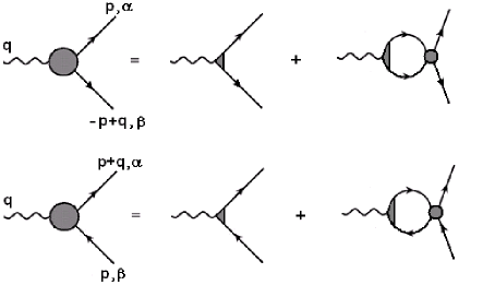
Figure 4: The Feynman diagrams for the three-legged response vertices associated with superconducting and density-wave orders.

Now, if we symmetrize the response vertices $\gamma^{\alpha\beta}_{SC}(\mathbf{p,q})$ and $\gamma^{\alpha\beta}_{DW}(\mathbf{p,q})$ with respect to their spin indices we obtain the following order parameters

$$\gamma_{SSC}(\mathbf{p,q})=\gamma^{\uparrow\downarrow}_{SC}(\mathbf{p,q})-\gamma^{\downarrow\uparrow}_{SC}(\mathbf{p,q})$$

$$\gamma_{TSC}(\mathbf{p,q})=\gamma^{\uparrow\downarrow}_{SC}(\mathbf{p,q})+\gamma^{\downarrow\uparrow}_{SC}(\mathbf{p,q})$$

$$\gamma_{SDW}(\mathbf{p,q})=\gamma^{\uparrow\uparrow}_{DW}(\mathbf{p,q})-\gamma^{\downarrow\downarrow}_{DW}(\mathbf{p,q})$$

$$\gamma_{CDW}(\mathbf{p,q})=\gamma^{\uparrow\uparrow}_{DW}(\mathbf{p,q})+\gamma^{\downarrow\downarrow}_{DW}(\mathbf{p,q})$$

where SSC and TSC correspond to singlet and triplet superconductivity and SDW and CDW stand for charge and spin density waves, respectively. Hence, using the above relations one can readily derive the RG flow equations for each response vertex associated with a potential instability of the normal state towards a given ordered (i.e. symmetry-broken) phase. The initial conditions for these RG flow equations will determine the symmetry of the order parameter. Thus

$$\gamma_{iR}(\mathbf{p,q};\Lambda=\Lambda_{0}) = 1\hskip 5.69046pt\textrm{($s$-wave)}$$

$$\gamma_{iR}(\mathbf{p,q};\Lambda=\Lambda_{0}) = \frac{1}{\sqrt{2}}(\cos p_{x}-\cos p_{y})\hskip 5.69046pt\textrm{($d_{x^{2}-y^{2}}$-wave)}$$

where $i=$ SSC, TSC, CDW and SDW. Once we computed the response vertices associated with these order parameters, we can now proceed to calculate their corresponding static susceptibilities. From Fig. 5, one can easily verify that they are given by

$$\Lambda\frac{d}{d\Lambda}\chi_{R,SC}(\mathbf{q}=0;\Lambda)=-\int\frac{d\mathbf{p}}{v_{F}(\mathbf{p})}[\gamma_{R,SC}(\mathbf{p,-p};\Lambda)]^{2}$$

$$\Lambda\frac{d}{d\Lambda}\chi_{R,DW}(\mathbf{q}=\mathbf{Q};\Lambda)=-\left(\frac{\Lambda}{\Lambda+2|\mu|}\right)\int\frac{d\mathbf{p}}{v_{F}(\mathbf{p})}$$

$$\hskip 113.81102pt\times[\gamma_{R,DW}(\mathbf{p+Q,p};\Lambda)]^{2}$$

where, to avoid cluttering up the notation too much, we simply write $SC$ for both singlet and triplet and $DW$ for charge and spin density wave susceptibilities. In addition, the vector $\mathbf{Q}=(\pi,\pi)$ is the commensurate antiferromagnetic wave vector.

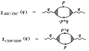
Figure 5: Feynman diagrams for the susceptibilities associated with both singlet and triplet superconductivity and charge and spin density wave orders.

III Numerical Results

To solve all these integro-differential RG equations numerically, we will follow the standard procedure of discretizing the full FS continuum into $N$ patches and then apply the fourth-order Runge-Kutta method. All numerical results in this paper will be presented for $N=32$. Despite this moderate choice of number of patches, we point out that our results show good convergence properties in the low-energy limit.

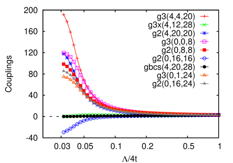
Figure 6: (Color online) The two-loop RG flow of the renormalized couplings (in units of $t$) for initial interaction $U=3t$ and $\mu=-0.05t$. We discretize the FS into $N=32$ patches, where 0, 8, 16, 24 represent the antinodal directions, and 4, 12, 20, 28 refer to the nodal points.

First, we focus our attention on the numerical solution of Eq. (8) for the renormalized couplings as a function of the ratio $\Lambda/4t$. As an initial condition for these equations, we choose the weak-to-moderate bare interaction $U=3t$. Our results are displayed in Fig. 6 for the case of $\mu=-0.05t$, which corresponds to a hole doping $x$ of approximately $x\approx 3.4\%$. In this regime, we observe that the inclusion of two-loop quantum fluctuations has important consequences to the flow of all couplings. Instead of exhibiting a divergence at a finite energy scale as obtained in several earlier one-loop RG investigations Zanchi ; Metzner ; Honerkamp , the couplings now display a tendency to level off in the low-energy limit. This result therefore implies that the two-loop RG corrections clearly diminish the importance of fluctuations as compared to the one-loop RG theory. It is true, however, that several (but not all) couplings become saturated at fairly strong-coupling fixed values. This is a well-known problem in RG theory and happens as well in other applications of this method to quantum field theories in which fluctuation effects are known to be very strong (the most notorious example being the Wilson-Fisher fixed point Wilson ; Brezin in $\phi^{4}$-theory at three dimensions). Nevertheless, the RG results in most cases are qualitatively correct even in a strong-coupling regime. The same is true in our case. When one of the renormalization couplings reaches an upper bound at the FS the whole flow is automatically stopped in spite of the fact that all couplings will not behave in the same way. We test the validity of our results by analyzing several physical quantities simultaneously. Until this critical RG scale is reached by one of the couplings, no unphysical trend is observed in our calculations. In view of this, we hope that our two-loop RG results will also capture at least qualitatively the most essential aspects of the physics of the 2D Hubbard model in the low-energy limit.

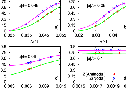
Figure 7: (Color online) The renormalized quasiparticle weight $Z_{\Lambda}(\mathbf{k})$ in the nodal and antinodal directions versus $\Lambda/4t$ for initial interaction $U=3t$ and initial condition $Z_{\Lambda_{0}=4t}(\mathbf{k})=1$: a) $|\mu|/t=0.045$, b) $|\mu|/t=0.05$, c) $|\mu|/t=0.08$ and d) $|\mu|/t=0.1$. The solid lines represent curve fittings of the RG data.

Next we present the results for the two-loop RG flow of the associated momentum-resolved quasiparticle weight $Z_{\Lambda}(\textbf{p})$. Here $Z_{\Lambda}(\textbf{p})$ is determined for several doping regimes as the low-energy limit is approached. The RG flows are displayed in Fig. 7 for the special choices of momentum at the nodal [near $(\pi/2,\pi/2)$] and antinodal [near $(\pi,0)$] directions. For doping levels up to a critical value $\mu_{c}=-0.045t$, corresponding to $x_{c}\approx 3\%$, we observe that the quasiparticle weights associated with both nodal and antinodal directions become strongly suppressed and eventually scale down to zero at sufficiently low-energy scales. This result in fact holds for all points of the underlying FS of the system. From the two-loop RG flows of the several order-parameter susceptibilities displayed in Figs. 8(a) and 8(b), we observe that the s-SDW is by far the dominant instability at these low doping values. From these two results we can infer that, for $|\mu|/t\leq 0.045$, the Fermi surface (if we define it simply as the locus in $\mathbf{k}$-space which exhibits a discontinuous jump in the momentum distribution function) is completely smeared out by interactions and the resulting ground state should be given by an antiferromagnetic insulator. This agrees for instance with the fact that, exactly at half-filling, this model is known to have an antiferromagnetic insulating ground state for any finite local interaction $U$. Our two-loop RG approach therefore successfully reproduces this important aspect of the problem.

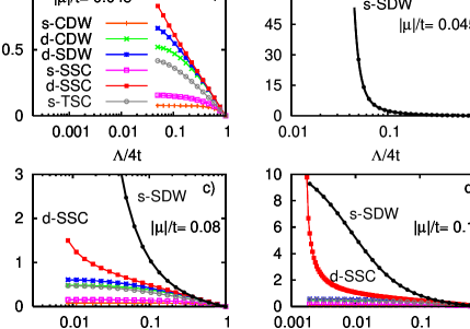
Figure 8: (Color online) The two-loop RG flows of several static order-parameter susceptibilities for initial interaction $U=3t$ with: a) and b) $|\mu|/t=0.045$, c) $|\mu|/t=0.08$ and d) $|\mu|/t=0.1$; CDW and SDW stand for charge and spin density waves; SSC and TSC stand for singlet and triplet superconductivity; the prefixes “s” and “d” refer to $s$-wave and $d_{x^{2}-y^{2}}$-wave symmetries.

Following this, we probe the system at a slightly larger hole doping regime, i.e. $\mu/t=-0.05$, which corresponds to $x\approx 3.4\%$. At this regime, we obtain that the quasiparticle gap immediately closes around the nodal directions but remains unaffected in the antinodal regions. The complete suppression of the spectral weight only in the antinodal zones suggests the existence of a NFL phase with quasiparticle-like excitations only around the nodal directions of the Fermi surface. From a technical point of view, this result originates from the anisotropy in the anomalous dimension $\eta(\mathbf{p})$ displayed in Eq. (LABEL:eta). This effect is to some extent reminiscent of the nodal-antinodal dichotomy and is in agreement with the general observation that, at light dopings, there are no coherent quasiparticle peaks at the antinodal points in the pseudogap phase of underdoped cuprates. However, we point out that the anisotropy obtained here in this work is still very small as compared with the experimental values observed in these materials. This is undoubtedly related to our choice of initial interaction $U=3t$. If we increase the on-site interaction of the model, we expect that this trend will be amplified further. This conjecture finds support in recent numerical results obtained from quantum cluster approaches Kyung for $U=8t$, where a stronger nodal-antinodal dichotomy is indeed observed in the model at finite doping.

Such a NFL character is observed here until the corresponding doping reaches $|\mu|/t=0.08$ (i.e. $x\approx 5.1\%$). At this hole doping, both the antinodal and nodal quasiparticle weights become nonzero even when we extrapolate our RG flow to very low $\Lambda/4t$ scales. This indicates that the resulting FS is fully reconstructed in this regime. Moreover, as shown in Fig. 8(c), we observe already the beginning of the unlimited growth of the $d_{x^{2}-y2}$-wave pairing instability in the presence of the still leading s-SDW susceptibility. This mixed d-SSC and s-SDW metallic state is observed until $|\mu|/t=0.1$ (i.e. $x\approx 6.2\%$). At this doping value, as indicated in Fig. 8(d), the d-SSC susceptibility finally overcomes the s-SDW and the system turns into a $d_{x^{2}-y^{2}}$-wave superconductor. As a consequence, we point out that this latter result adds further support to the possible existence of a $d_{x^{2}-y^{2}}$-wave superconducting state in the 2D Hubbard model as was first obtained in Refs. Zanchi ; Metzner ; Honerkamp within a one-loop RG scheme.

One important point we would like to emphasize here is that, for doping regimes satisfying $|\mu|\leq 0.08t$, the dominant fluctuations in our results are always of s-SDW type (i.e. antiferromagnetism), in qualitative agreement with several previous studies focusing on this model Maier ; Zanchi ; Metzner ; Honerkamp . This result therefore favors the interpretation that the driving mechanism underlying our NFL evidence should be mediated by antiferromagnetic spin-fluctuations.

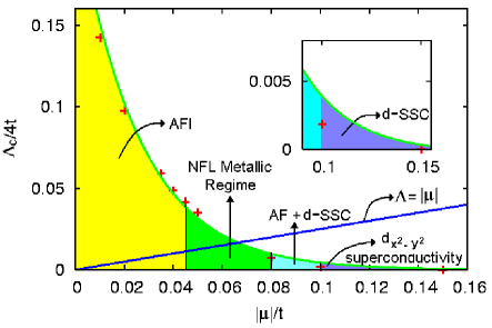
Figure 9: (Color online) Two-loop RG phase diagram for the 2D Hubbard model as a function of the critical RG scale $\Lambda_{c}$ and the hole doping $\mu$ for local on-site bare interaction $U=3t$.

We summarize our results displaying in Fig. 9 a two-loop RG phase diagram of the 2D Hubbard model as a function of both a critical RG scale $\Lambda_{c}$ and the hole doping represented by $\mu$. This phase diagram however must be interpreted only qualitatively since the numerical determination of the exact critical scale where the order-parameter susceptibilities truly diverge is of course very difficult and, for this reason, this is always based on a chosen criterion. Therefore, as we saw before, we find evidence of an extended antiferromagnetic insulating (AFI) phase from half-filling up to $|\mu|/t=0.045$. For $0.045\leq|\mu|/t\leq 0.08$, we obtain instead that the formation of a NFL metallic phase with a truncated Fermi surface in the nodal regions is favored. For $0.08\leq|\mu|/t\leq 0.1$, the FS is fully restored with the resulting metallic state displaying enhanced antiferromagnetic and $d_{x^{2}-y2}$-wave pairing correlations. Finally, for $|\mu|/t\geq 0.1$, the system shows a $d_{x^{2}-y2}$-wave superconducting phase. Moreover, if we suppose that it is possible to associate the RG scale $\Lambda_{c}$ with an effective critical temperature scale $T_{c}$, this could in principle provide approximate estimates of the critical temperatures for the various phase transitions displayed by this model obtained within our two-loop RG scheme. Following this approach, we obtain that, for the $d_{x^{2}-y2}$-wave superconducting phase, the highest effective critical temperature scale displayed in our two-loop RG phase diagram is given by the curve fitting value $\Lambda_{c}/4t\approx 0.004t$ (see inset), which is surprisingly in qualitative agreement with the result $T_{c}\approx 0.023t$ obtained in the literature for $U=4t$ within quantum cluster methods Maier .

IV Conclusion

We have analyzed the 2D Hubbard model starting from weak-to-moderate couplings by implementing a functional generalization of the field-theoretical renormalization group approach up to two-loop order. Our calculations here were mainly restricted to the limit of $T\rightarrow 0$, i.e. to the analysis of the universal ground state properties and its low-lying excitations, as a function of doping. The two-loop RG scheme was necessary in order to discuss the effect of the momentum-resolved anomalous dimension $\eta(\textbf{p})$, which shows up in the normal phase of the model on the corresponding low-energy single-particle excitations. As a result, we have found evidence for an extended antiferromagnetic insulating (AFI) ground state in the vicinity of half-filling. This result was particularly encouraging since it agrees with the fact that, exactly at half-filling, this model is known to produce an AFI ground state for any finite local interaction $U$. Our two-loop RG approach therefore successfully reproduced this important aspect of the problem.

For a slightly higher doping regime, we have obtained that the formation of a NFL metallic phase with a truncated Fermi surface in the nodal regions was favored. This effect is originated by the anisotropy of the momentum-resolved anomalous dimension $\eta(\textbf{p})$ at this regime and it is reminiscent, to some extent, of the nodal-antinodal dichotomy observed in the pseudogap phase in underdoped cuprates. However, the anisotropy found here was still very small compared with the experimental values observed in those materials. This is undoubtedly related to our choice of initial interaction $U=3t$. If we increase the on-site interaction of the model, we expect that this trend will be amplified further. Such a NFL character was observed for a finite doping range, after which both nodal and antinodal quasiparticle weights became nonzero even when we extrapolated our RG flow to very low RG scales. This indicated that the resulting FS, in this new phase, was fully reconstructed. With further doping, the system finally developed a $d_{x^{2}-y^{2}}$-wave pairing instability in the low-energy limit. This suggests the formation of $d_{x^{2}-y^{2}}$-wave superconducting ground state sufficiently away from half-filling. This latter two-loop RG result therefore adds further support to the still much-debated existence of a $d_{x^{2}-y^{2}}$-wave superconducting phase in the 2D Hubbard model and this is in qualitative agreement with the first results obtained in Refs. Zanchi ; Metzner ; Honerkamp within a one-loop RG scheme.

Since our two-loop RG results have several analogies with the observed phenomena in the high-Tc superconductors, a few remarks are in order. These materials are known to be Mott insulators at half-filling regime. This unambiguously implies that the strong-coupling regime should be an important ingredient to describe quantitatively their observed properties. The main aim of this work however was not to achieve quantitative agreement with the experimental results. Our objective was to show that even the simplest version of the 2D Hubbard model is rich enough to capture some of the main features displayed by those materials. In order to describe quantitatively the experimental results of the high-Tc cuprates, it is essential to choose initial couplings larger than the ones considered in this work. Moreover, we should also take into account the effects produced by next nearest neighbor hoppings $t^{\prime}$ and $t^{\prime\prime}$. Nevertheless, it is reasonable to expect that, at least for the interaction strengths that apply to these compounds, the inclusion of $t^{\prime}$ and $t^{\prime\prime}$ in the Hamiltonian should not alter qualitatively the low-energy dynamics of the system. In this sense, it is reasonable to suppose that the cuprates could be potentially associated with a universality class which is well captured by our model. As we have shown here, even our simple version of the 2D Hubbard model already displays some important and nontrivial aspects of the physics exhibited by these materials.

On the other hand, there are still some open issues which were not addressed in this work. How the renormalization of the FS induced by interactions affects the RG flow is still not considered in our RG scheme. In recent years, there has been some progress in analyzing this problem in quasi-one dimensional systems Ledowski ; Ledowski2 . However, a two-loop RG calculation of this effect in two-dimensional systems still remains a very difficult task and, to our knowledge, has not been calculated so far. Another important aspect which deserves future investigation concerns the actual importance of quantum fluctuations beyond the two-loop RG level for this model. Since three-loop RG calculations do not seem to be an easy prospect in the near future, we can nevetherless learn a lot about this question by comparing one-loop with two-loop RG calculations. One important result obtained here was the certainty that one-loop RG calculations in general tend to overestimate the effect of fluctuations near half-filling. As a result, our two-loop RG theory yields a better controlled approximation in the low-energy limit for this doping regime. In addition, our results suggest that the pseudogap phase might be indeed related to a strong-coupling regime in the model. However, like any other strong-coupling problem in correlated systems, it is still not easy to have full analytical control in such case. In other words, there is still room for improvement before one can claim to have a complete theory for the strong-coupling regime of the 2D Hubbard model. However, given our encouraging results so far, we believe our two-loop RG approach could provide a good basis for a complementary view of this important problem starting from a weak-to-moderate coupling perspective.

Note added - Recently, we learned about a related study in the context of the 2D $t-t^{\prime}$ Hubbard model, Ref. Katanin2 .

- (1) J. Orenstein, and A. J. Millis, Science 288, 468 (2000).
- (2) T. Timusk, and B. Statt, Rep. Prog. Phys. 62, 61 (1999).
- (3) M. R. Norman, D. Pines and C. Kallin, Adv. Phys. 54, 715 (2005).
- (4) N. Doiron-Leyraud, C. Proust, D. LeBoeuf, J. Levallois, J.-B. Bonnemaison, R. Liang, D. A. Bonn, W. N. Hardy, and L. Taillefer, Nature 447, 565 (2007).
- (5) H. Ding, T. Yokoya, J. C. Campuzano, T. Takahashi, M. Randeria, M. R. Norman, T. Mochiku, K. Kadowakia, and J. Giapintzakis, Nature (London) 382, 51 (1996).
- (6) A. G. Loeser, Z.-X. Shen, D. S. Dessau, D. S. Marshall, C. H. Park, P. Fournier, and A. Kapitulnik, Science 273, 325 (1996).
- (7) K. M. Shen, F. Ronning, D. H. Lu, F. Baumberger, N. J. C. Ingle, W. S. Lee, W. Meevasana, Y. Kohsaka, M. Azuma, M. Takano, H. Takagi, and Z. -X. Shen, Science 307, 901 (2005).
- (8) K. Tanaka, W. S. Lee, D. H. Lu, A. Fujimori, T. Fujii, Risdiana, I. Terasaki, D. J. Scalapino, T. P. Devereaux, Z. Hussain, and Z.-X. Shen, Science 314, 1910 (2006).
- (9) P. W. Anderson, Science 235, 1196 (1987).
- (10) Th. Maier, M. Jarrell, Th. Pruschke, and J. Keller, Phys. Rev. Lett. 85, 1524 (2000); T. A. Maier, M. Jarrell, T. C. Schulthess, P. R. C. Kent, and J. B. White, Phys. Rev. Lett. 95, 237001 (2005).
- (11) B. Kyung, S. S. Kancharla, D. Senechal, A. M. S. Tremblay, M. Civelli, and G. Kotliar, Phys. Rev. B 73, 165114 (2006).
- (12) D. Zanchi, and H. J. Schulz, Phys. Rev. B 54, 9509 (1996); 61, 13609 (2000).
- (13) C. J. Halboth, and W. Metzner, Phys. Rev. B 61, 7364 (2000); Phys. Rev. Lett. 85, 5162 (2000).
- (14) C. Honerkamp, M. Salmhofer, N. Furukawa, and T. M. Rice, Phys. Rev B 63, 35109 (2001).
- (15) R. Shankar, Rev. Mod. Phys. 66, 129 (1994).
- (16) P. Kopietz, and T. Busche, Phys. Rev. B 64, 155101 (2001).
- (17) S. W. Tsai, and J. B. Marston, Can. J. Phys. 79, 1463 (2001).
- (18) J. Gonzalez, F. Guinea, and M. A. H. Vozmediano, Phys. Rev. Lett. 79, 3514 (1997).
- (19) B. Binz, D. Baeriswyl, and B. Doucot, Eur. Phys. J. B 25, 69 (2002).
- (20) A. Ferraz, Phys. Rev. B 68, 075115 (2003).
- (21) D. Zanchi, Europhys. Lett. 55, 376 (2001); L. Arrachea, and D. Zanchi, Phys. Rev. B 71, 064519 (2005).
- (22) C. Honerkamp, and M. Salmhofer, Phys. Rev. B 67, 174504 (2003).
- (23) A. A. Katanin, and A. P. Kampf, Phys. Rev. Lett. 93, 106406 (2004).
- (24) D. Rohe, and W. Metzner, Phys. Rev. B 71, 115116 (2005).
- (25) Non-conserving many-body approximations in turn may lead to the violation of exact results such as Ward identities.
- (26) H. Freire, E. Correa, and A. Ferraz, Phys. Rev. B 71, 165113 (2005).
- (27) M. E. Peskin and D. V. Schroeder, An Introduction to Quantum Field Theory (Perseus, Cambridge, 1995).
- (28) S. Weinberg, The Quantum Theory of Fields (Cambridge University, Cambridge, England, 1996), Vol. II.
- (29) See, e.g., J. Solyom, Adv. Phys. 28, 201 (1979).
- (30) For a two-loop RG calculation of the response functions in the context of a simpler 2D flat FS model, see E. Correa, H. Freire, and A. Ferraz, arXiv:cond-mat/0512626 (unpublished).
- (31) K. G. Wilson and M. E. Fisher, Phys. Rev. Lett. 28, 240 (1972).
- (32) The systematic study of higher-order corrections in the -expansion was performed in: E. Brezin, J. C. Le Gillou and J. Zinn-Justin, Phys. Rev D 9, 1121 (1974).
- (33) S. Ledowski, P. Kopietz, and A. Ferraz, Phys. Rev. B 71, 235106 (2005).
- (34) S. Ledowski, and P. Kopietz, Phys. Rev. B 76, 121403(R) (2007).
- (35) A. A. Katanin, arXiv:0806.0300 (unpublished).