Some aspects of extreme value statistics under serial dependence

Abstract

On the occasion of Laurens de Haan’s 70th birthday, we discuss two aspects of the statistical inference on the extreme value behavior of time series with a particular emphasis on his important contributions. First, the performance of a direct marginal tail analysis is compared with that of a model-based approach using an analysis of residuals. Second, the importance of the extremal index as a measure of the serial extremal dependence is discussed by the example of solutions of a stochastic recurrence equation.

AMS subject classification: primary 62G32; secondary 60G70, 62M10

Key words and phrases: extremal index, extreme quantile, extreme value index, linear time series, mixing condition, model deviation, robustness, tail analysis

1 Introduction

Since the publication of his Ph.D.-thesis, Laurens de Haan has been one of the main driving forces behind the impressive development of extreme value statistics in the last four decades. While he is best known for his seminal contributions to extreme value theory for i.i.d. samples of univariate and multivariate observations and, in recent years, for i.i.d. copies of continuous stochastic processes, he has also strongly influenced the extreme value theory (and practice) for serially dependent data in two ways: first by direct contributions, and second indirectly by promoting general principles. In the present paper, both aspects of the impact of Laurens de Haan’s work on the development of extreme value statistics for time series are discussed.

Throughout his work, Laurens de Haan has always aimed at the greatest (reasonable) generality of the models under consideration. For example, while in many articles on univariate extreme value statistics it was assumed that exact generalized Pareto random variables (r.v.s), respectively, generalized extreme value r.v.s were observed, typically he only assumed that the underlying distribution belongs to the domain of attraction of some extreme value distribution. Under this much more general condition, he analyzed the consequences of this deviation from the ideal situation. The second order condition, de Haan and Stadtmüller (1996) introduced and analyzed for that purpose, is now the generally accepted standard condition in this field (cf. (2.4) for a simplified version). (It is worth mentioning that essentially the same condition has been independently suggested by Pereira (1994).) Similarly, also in de Haan’s work on multivariate extreme value statistics it is not assumed that the observations are drawn from an exact extreme value distribution, but only that the underlying distribution belongs to the domain of attraction of such a distribution. Moreover, he always preferred weak smoothness conditions on the exponent measure pertaining to this multivariate extreme value distribution to restrictive parametric submodels of the natural infinite-dimensional extreme value model. With the improvement of the resulting nonparametric methods, in the last couple of years this approach has become more widely accepted as a reliable tool, that is more robust than parametric approaches.

The extreme value estimators, that were suggested and analyzed for univariate i.i.d. samples by Laurens de Haan and many others, can also be used for the marginal tail analysis of stationary time series, but often their performance deteriorates because of the serial dependence between the observations. Therefore, in contrast to the aforementioned general trend towards weak model assumptions, in the literature on extreme value statistics for time series (and particularly linear time series) often an approach is favored in which a parametric serial dependence structure is assumed and estimators are considered which are based on a tail analysis of the (nearly independent) residuals after the parametric model has been fitted. In the main Section 2, we will reassess some of the results which seemingly show the underperformance of a direct extreme value analysis, that only requires weak nonparametric assumptions on the dependence structure, relative to the model-based approach.

Often one is interested not only in the marginal tail behavior but also in the extremal dependence structure. The literature on the dependence analysis is strongly dominated by the problem of estimating the extremal index, that describes the influence of the serial dependence on the asymptotic behavior of maxima of consecutive observations. It is somewhat surprising that, while in the last two decades statistical methods which are based on exceedances (or order statistics) instead of block maxima have become much more popular, this shift of focus is not reflected in the statistical theory of the extremal dependence structure. In Section 3, we will argue that the statistical inference of the extremal dependence structure should be put on a broader basis and exemplify this claim by the asymptotic behavior of naturally arising statistics that were analyzed by Laurens de Haan and co-authors in a specific time series model.

Obviously, the extreme value statistics of time series is a field of research much too broad and diverse to be reviewed in a short article. For that reason, we decided to focus on the two above topics, knowing that this selection is largely a matter of taste. Important subfields which we will not discuss at all are, for instance, the extreme value inference under additional structural assumptions (e.g. for Markov chains) and the analysis of nonstationary or multivariate time series, among many other topics. We will also not discuss Laurens de Haan’s contributions to the extreme value theory of continuous time processes, since he usually assumes that i.i.d. copies of the whole process are observed. Consequently, this theory is a natural extension of the theory for multivariate observations rather than the theory for time series and will thus be discussed in Michael Falk’s contribution to this volume.

Throughout this article, we will assume that $X_{t}$, $t\in{\mathbb{Z}}$, is a stationary time series with marginal distribution function (d.f.) $F_{X}$, that belongs to the domain of attraction of some extreme value distribution.

2 Marginal tail analysis: In models we trust?

In this section we assume that only the tail behavior of the stationary marginal d.f. $F_{X}$ is to be analyzed. To this end, estimators of tail parameters based on exceedances over high thresholds can be used which were developed for i.i.d. observations, but the serial dependence must be taken into account when the accuracy of these estimators is assessed (e.g. to construct confidence intervals).

Roughly speaking, one can distinguish three different approaches:

1. One tries to identify independent clusters of exceedances and constructs a new data set by taking one observation (usually the cluster maximum) from each cluster. This way one obtains an i.i.d. sample whose tail behavior can be analyzed using standard techniques from classical extreme value statistics for i.i.d. data.

2. In a nonparametric approach, one may also apply the classical tail estimators (originally proposed for i.i.d. samples) directly to all exceedances observed in the time series. However, if one wants to construct confidence intervals, then one needs results on their asymptotic behavior that hold true under mild assumptions on the serial dependence structural.

3. Finally, in a semiparametric fashion, one can fit a parametric model of the serial dependence to the data and then one can try to infer the tail behavior of the time series from a suitable analysis of the residuals. This approach seems best suited for heavy-tailed linear time series for which the relationship between the tail of the stationary distribution and the tail of the distribution of the innovations is particularly simple.

The declustering approach (i) is most appropriate if the time series consists of clearly separable, short clusters of extreme events, that preferably have a “physical” interpretation. Nice examples are data sets of wave heights and other quantities describing sea conditions that were analyzed by Laurens de Haan and co-authors in several publications. For example, starting with wave heights, wave periods and still water levels that were observed every 3 hours at some point near the Dutch coast, de Haan and de Ronde (1998) obtained nearly i.i.d. data by only considering the maximum of each coordinate in each storm. See Dekkers and de Haan (1989), and de Haan (1990) for further examples of that type.

Unfortunately, in many applications either it is difficult to identify independent clusters of extremes, or the clusters are large so that it would be a great waste of information to use but one observation in each cluster. For example, time series of returns of some financial investment often exhibit long periods of high volatility during which several dependent exceedances occur. Moreover, declustering schemes often depend on certain subjective choices, and usually the influence of these choices on the accuracy of the tail analysis is difficult to assess. (A first trial to overcome these problem was made by Ledford and Tawn (2003).)

For these reasons, in the sequel we will focus on the nonparametric approach (ii) and the model-based semiparametric approach (iii). In particular, we will compare the accuracy and the robustness of resulting estimators of extreme quantiles in the case of heavy-tailed linear time series.

2.1 Direct extreme value analysis

Among all tail estimators, the asymptotic behavior of the Hill estimator

$$\hat{\gamma}_{n,k}:=\frac{1}{k}\sum_{i=1}^{n}\log\frac{X_{n-i+1:n}}{X_{n-k:n}}$$

under serial dependence has been studied most thoroughly in literature; here $X_{j:n}$ denotes the $j$th smallest order statistic of $X_{1},\ldots,X_{n}$. One of the first references is an unpublished manuscript by Rootzén, Leadbetter and de Haan (1990), in which the asymptotic normality of the Hill estimator is established under quite weak conditions, including strong mixing of the time series. At about the same time, Hsing (1991) independently proved the asymptotic normality of the Hill estimator under comparable, but different structural assumptions on the serial dependence. Since then, the limit distribution of (variants of) the Hill estimator under serial dependence has been examined in several papers; see, e.g., Resnick and Stărică (1997) and Novak (2002).

Of course, in most applications, the extreme value index is not the primary object of interest, but for instance exceedance probabilities or extreme quantiles are to be estimated. Consequently, Rootzén, Leadbetter and de Haan (1990) also examined the asymptotic behavior of extreme quantile estimators. Moreover, more general statistics of the type

$$\sum_{i=1}^{n}\phi_{n}\big{(}(X_{i}-u_{n})^{+}\big{)}$$

(with suitable functions $\phi_{n}$) were considered, which are nowadays known as tail array sums. The asymptotic theory of tail array sums was further developed by Leadbetter and Rootzén (1993) and Leadbetter (1995). In a final version, this part of the manuscript was published in the article Rootzén, Leadbetter and de Haan (1998).

The general results about the asymptotic normality of tail array sums proved a powerful tool. In particular, Rootzén (1995), who established the weak convergence of the empirical process

$$e_{n}(x)=\frac{1}{\sqrt{n\bar{F}_{X}(u_{n})}}\sum_{i=1}^{n}\Big{(}1_{\{X_{i}>\sigma_{n}x+u_{n}\}}-\bar{F}_{X}(\sigma_{n}x+u_{n})\Big{)}$$

(with $\bar{F}_{X}=1-F_{X}$) towards a Gaussian process under $\beta$-mixing (absolute regularity) of the time series, used this result to verify the convergence of the finite dimensional marginal distributions. (In the improved version Rootzén (2006), a similar result is also established under the weaker assumption that the time series is strongly mixing.) Using this convergence, Drees (2000) proved a weighted approximation of the pertaining tail quantile process, from which one can easily conclude the asymptotic normality of a general class of estimators of the extreme value index or of estimators of extreme quantiles; cf. Drees (2000,2002,2003).

2.2 Model-based tail estimators

Here we focus on linear time series models, because for this class the semiparametric model-based approach seems particularly promising. More precisely, we assume that the time series allows a representation as a moving average of infinite order:

$$X_{t}=\sum_{j=-\infty}^{\infty}\psi_{j}Z_{t-j},\qquad t\in{\mathbb{Z}}.$$ (2.1)

Moreover, the i.i.d. innovations $Z_{t}$ are assumed to have balanced heavy tails, i.e. their survival function $\bar{F}_{Z}$ satisfies

$$\bar{F}_{Z}(x)=x^{-1/\gamma}L(x),\qquad\lim_{x\to\infty}\frac{\bar{F}_{Z}(x)}{\bar{F}_{|Z|}(x)}=p$$ (2.2)

for some $\gamma>0$, $p\in(0,1]$ and some slowly varying function $L$. Mikosch and Samorodnitsky (2000) proved that

$$\lim_{x\to\infty}\frac{\bar{F}_{X}(x)}{\bar{F}_{Z}(x)}=\frac{1}{p}\sum_{j=-\infty}^{\infty}\Big{(}p\psi_{j}^{1/\gamma}1_{\{\psi_{j}>0\}}+(1-p)|\psi_{j}|^{1/\gamma}1_{\{\psi_{j}<0\}}\Big{)}$$ (2.3)

if $0<\sum_{j=-\infty}^{\infty}\psi_{j}^{2}<\infty$ for $\gamma<1/2$, and $0<\sum_{j=-\infty}^{\infty}|\psi_{j}|^{1/\gamma-{\varepsilon}}<\infty$ for some $\varepsilon>0$ in the case $\gamma\geq 1/2$, and if $E(Z_{t})=0$ for $\gamma<1$. (Under stronger conditions, similar results were already established by Davis and Resnick (1985) and Datta and McCormick (1998), among others.)

In particular, the time series has the same extreme value index $\gamma$ as the innovations. Hence, if one has estimated the coefficients $\psi_{j}$ and the time series model is invertible, then it suggest itself to estimate $\gamma$ by applying the Hill estimator (or some other estimator of the extreme value index) to the resulting residuals $\hat{Z}_{t}$, which are approximately i.i.d. Moreover, if $p$ (or some estimate of it) is known, one may even calculate estimates of exceedance probabilities $\bar{F}_{X}(x)$ over high thresholds $x$ or estimators of extreme quantiles $F_{X}^{-1}(1-t)$ (for small $t>0$) from estimators of the corresponding quantities of the d.f. $F_{Z}$ of the innovations, which in turn can be obtained from a tail analysis of the residuals. This program has been worked out for the first time by Resnick and Stărică (1997) for the Hill estimator and autoregressive time series $AR(m)$ of order $m<\infty$:

$$X_{t}=\sum_{i=1}^{m}\varphi_{i}X_{t-i}+Z_{t},\quad t\in{\mathbb{Z}}.$$

Let $\hat{\varphi}_{i}$, $1\leq i\leq m$, be estimators of the coefficients such that $d_{n}(\hat{\varphi}_{i}-\varphi_{i})_{1\leq i\leq m}$ converges to some nondegenerate distribution; here $d_{n}\rightarrow\infty$ determines the rate of convergence of the estimators $\hat{\varphi}_{i}$. Define the residuals

$$\hat{Z}_{t}:=X_{t}-\sum_{i=1}^{m}\hat{\varphi}_{i}X_{t-i},\qquad m+1\leq t\leq n.$$

Resnick and Stărică (1997) proved that the Hill estimator based on the absolute residuals

$$\hat{\gamma}_{n,|Z|}:=\frac{1}{k}\sum_{i=1}^{k}\log\frac{|\hat{Z}|_{n-m-i+1:n-m}}{|\hat{Z}|_{n-m-k:n-m}}$$

(with $|\hat{Z}|_{j:n-m}$ denoting the $j$th smallest order statistic of $|Z_{t}|$, $m-1\leq t\leq n$) is asymptotically normal

$$\sqrt{k}\big{(}\hat{\gamma}_{n,|Z|}-\gamma\big{)}\;\longrightarrow\mathcal{N}_{(0,\gamma^{2})}$$

weakly, provided that the d.f. $F_{|Z|}$ of the absolute innovations satisfies the second order condition

$$\lim_{t\to\infty}\frac{\displaystyle\frac{\bar{F}_{|Z|}(tx)}{\bar{F}_{|Z|}(t)}x^{1/\gamma}-1}{\tilde{A}(t)}=\frac{x^{\tilde{\rho}}-1}{\tilde{\rho}}$$ (2.4)

for some $\tilde{\rho}\leq 0$, and the number $k$ of order statistics used for estimation tends to $\infty$ sufficiently slowly such that

$$\lim_{n\to\infty}\sqrt{k}\tilde{A}\big{(}F^{-1}_{|Z|}(1-k/n)\big{)}=0$$ (2.5)

and

$$\lim_{n\to\infty}\frac{\displaystyle\sqrt{k}F^{-1}_{|Z|}(1-\sqrt{k}/n)}{\displaystyle d_{n}F^{-1}_{|Z|}(1-k/n)}=0.$$ (2.6)

(Ling and Peng (2004), who established a similar result for ARMA time series, showed that condition (2.6) is not needed if $d_{n}$ equals the best attainable rate.)

In contrast, the Hill estimator applied to the absolute observations $|X_{t}|$ directly is asymptotically normal with asymptotic variance

$$\gamma^{2}\bigg{(}1+2\frac{\sum_{j=1}^{\infty}\sum_{i=0}^{\infty}\min\big{(}|\psi_{j}|^{1/\gamma},|\psi_{i+j}|^{1/\gamma}\big{)}}{\sum_{i=0}^{\infty}|\psi_{j}|^{1/\gamma}}\bigg{)}$$ (2.7)

with $\psi_{i}$ denoting the coefficients of the $MA(\infty)$-representation of the time series, i.e. $X_{t}=\sum_{i=0}^{\infty}\psi_{i}Z_{t-i}$, provided that the d.f. $F_{|X|}$ of the absolute observations and the sequence of numbers of order statistics used for estimation satisfy the analogs to the conditions (2.4) and (2.5). Note that the asymptotic variance (2.7) of the Hill estimator directly applied to the absolute values of the observations is strictly larger than the asymptotic variance $\gamma^{2}$ of the Hill estimator based on the absolute residuals. For example, if one considers an $AR(1)$ time series with coefficient $\varphi_{1}\in(-1,1)$, then $\psi_{i}=\varphi_{1}^{i}$, $i\in{\mathbb{N}}_{0}$, and the asymptotic variance (2.7) equals $\gamma^{2}(1+|\varphi_{1}|^{1/\gamma})/(1-|\varphi_{1}|^{1/\gamma})$. Therefore, Resnick and Stărică (1997) claimed that “the procedure of applying the Hill estimator directly to an autoregressive process is less efficient than the procedure of first estimating autoregressive coefficients and then estimating $\alpha$” ($=1/\gamma$) “using estimated residuals”. This conclusion, however, is justified in general only if both Hill estimators use the same number of order statistics. Since the optimal numbers of order statistics used by the Hill estimators are essentially determined by the functions $\tilde{A}$ occurring in the second order condition (2.4) for $F_{|Z|}$ (in the case of the residual-based estimator) and $A$ in the analog condition for the absolute time series (for the directly applied Hill estimator), it is a priori unclear which of the estimators has the smaller variance when they both use an appropriate number of order statistics. Indeed, if the second order parameter$\tilde{\rho}$ is smaller in absolute value than the analogous parameter $\rho$ from the second order condition for $F_{|X|}$, then the best rate of convergence that can be achieved by the residual-based Hill estimator is of lower order than the optimal rate of the directly applied Hill estimator, i.e. the former estimator has asymptotic efficiency 0 with respect to the latter estimator. Conversely, if $|\tilde{\rho}|>|\rho|$ then the directly applied Hill estimator is asymptotically inefficient w.r.t. the model-based estimator, if both use the optimal number of order statistics.

For general linear time series, it is not known how the second order behavior of $F_{|X|}$ is related to the second order behavior of $F_{|Z|}$. However, for first order moving averages the relationship has been discussed by Geluk, Peng and de Vries (2000) and Geluk and Peng (2000), and the same technique can be used for finite order moving averages. For general linear dependence structures but a rather particular class of distributions of innovations, the relationship can be deduced from results by Barbe and McCormick (2004). More precisely, assume that

$$\bar{F}_{Z}(x)=x^{-1/\gamma}(c+dx^{-1}+o(x^{-1})),\quad F_{Z}(-x)=x^{-1/\gamma}(\tilde{c}+\tilde{d}x^{-1}+o(x^{-1}))$$

as $x\to\infty$. Then, by Section 2.1 of Barbe and McCormick (2004), the tail of the linear time series (2.1) behaves asymptotically as

$$F_{X}(x) = x^{-1/\gamma}(d_{\psi}+D_{\psi}x^{-1}+o(x^{-1}))\quad\text{with}$$

$$d_{\psi} = \sum_{j=-\infty}^{\infty}\Big{(}c\psi_{j}^{1/\gamma}1_{\{\psi_{j}>0\}}+\tilde{c}|\psi_{j}|^{1/\gamma}1_{\{\psi_{j}<0\}}\Big{)},$$

$$D_{\psi} = \sum_{j=-\infty}^{\infty}\Big{(}cd\psi_{j}^{1/\gamma+1}1_{\{\psi_{j}>0\}}+\tilde{c}\tilde{d}|\psi_{j}|^{1/\gamma+1}1_{\{\psi_{j}<0\}}\Big{)}.$$

Hence, for this type of innovations, both functions $A(t)$ and $\tilde{A}(t)$ are multiples of $t^{-1}$, but the constant factors differ from each other. Note that the above expansion of $\bar{F}_{Z}$ is equivalent to $F_{Z}^{-1}(1-t)=c^{\gamma}t^{-\gamma}+\gamma d+o(1)$, i.e., up to terms of smaller order the tails behave like those of a shifted Pareto distribution. This shows that indeed the result by Barbe and McCormick describes the relationship between the second order behavior of the tails of $F_{Z}$ and $F_{X}$ (or of $F_{|Z|}$ and $F_{|X|}$) only for a rather limited family of distributions of innovations.

To sum up, in general, the result by Resnick and Stărică (1997) does not allow to compare the asymptotic performance of the direct nonparametric approach and the model-based estimator if both use an appropriate number of order statistics.

Having said that, it is nevertheless plausible to expect that the residual-based estimator has a smaller variance if the extra factor by which $\gamma^{2}$ is multiplied in the variance formula (2.7) is much larger than 1 (e.g. if the absolute coefficient of an $AR(1)$ time series is close to 1). However, even in that case, the model based approach has serious drawbacks:

• As mentioned before, usually one is not mainly interested in the extreme value index but e.g. in exceedance probabilities $\bar{F}_{X}(x)$ (or extreme quantiles). To estimate such quantities, one uses the relationship (2.3) which may introduce a non-negligible additional error term if for the given threshold $x$ the ratio $\bar{F}_{X}(x)/\bar{F}_{Z}(x)$ is poorly approximated by the right hand side of (2.3).

• Of course, the model-based approach makes sense only if the model assumptions are (approximately) fulfilled. Although this remark is almost trivial, it is nevertheless crucial to be aware of the fact that even moderate deviations from the linear relationship between $X_{t}$ and $X_{t-1},\ldots,X_{t-m}$, which can hardly be detected by statistical tests, may completely wreck up the residual-based estimator, as we will see in the next subsection.

2.3 Comparison of model-based and direct extreme quantile estimators: a simulation study

Here we assume that $X_{t}$, $t\in\mathbb{Z}$, is a stationary $AR(1)$ time series, i.e. $X_{t}=\varphi_{1}X_{t-1}+Z_{t}$ with i.i.d. innovations $Z_{t}$ satisfying (2.2), and that an extreme quantile $F^{-1}_{X}(1-t)$ ($t>0$ small) is to be estimated. In this case relation (2.3) reads as

$$\lim_{x\to\infty}\frac{\bar{F}_{X}(x)}{\bar{F}_{Z}(x)}=\left\{\begin{array}[]{lcl}1/(1-\varphi_{1}^{1/\gamma}),&&\varphi_{1}\in[0,1),\\ \big{(}1+|\varphi_{1}|^{1/\gamma}(1-p)/p\big{)}/(1-|\varphi_{1}|^{2/\gamma}),&&\varphi_{1}\in(-1,0).\end{array}\right.$$ (2.8)

For simplicity (and in favor of the model-based approach) we assume that $p$ is known to be equal to $1/2$, so that (2.8) simplifies to

$$\lim_{x\to\infty}\frac{\bar{F}_{X}(x)}{\bar{F}_{Z}(x)}=1/(1-|\varphi_{1}|^{1/\gamma}),$$

which, by the regular variation of $\bar{F}_{Z}$, is equivalent to the following relationship between the corresponding quantile functions:

$$\lim_{t\downarrow 0}\frac{F_{X}^{-1}(1-t)}{F_{Z}^{-1}\big{(}1-(1-|\varphi_{1}|^{1/\gamma})t\big{)}}=1.$$

Hence, in the model-based approach one may estimate $F^{-1}_{X}(1-t)$ as follows:

• Estimate $\varphi_{1}$, e.g., by the sample auto-correlation $\hat{\varphi}_{1}$ at lag 1.

• Approximate $F^{-1}_{X}(1-t)$ by $F^{-1}_{Z}\big{(}1-(1-|\hat{\varphi}_{1}|^{1/\gamma})t\big{)}$ and estimate the latter by the Weissman estimator

  $$\hat{Z}_{n-k:n-1}\bigg{(}\frac{n(1-|\hat{\varphi}_{1}|^{1/\hat{\gamma}_{n,Z}})t}{k}\bigg{)}^{\hat{\gamma}_{n,Z}}$$

  where $\hat{Z}_{j:n-1}$ is the $j$th smallest order statistic of the residuals $\hat{Z}_{t}=X_{t}-\hat{\varphi}_{1}X_{t-1}$, $2\leq t\leq n$, and

  $$\hat{\gamma}_{n,Z}:=\frac{1}{k}\sum_{i=1}^{k}\log\frac{\hat{Z}_{n-i:n-1}}{\hat{Z}_{n-k-1:n-1}}$$

  is the corresponding Hill estimator. (The Weissman estimator can be motivated either by a Generalized Pareto approximation of $F_{Z}$ or the regular variation of $F^{-1}_{Z}$ which implies $F^{-1}_{Z}(1-u)\approx F^{-1}_{Z}(1-k/n)(nu/k)^{-\gamma}$ for sufficiently small $u$ and $k/n$.)

In a small simulation study we consider time series of length $n=2000$ with $\varphi_{1}=0.8$ and two different symmetric distributions of the innovations $Z_{t}$:

1. a double-sided (unshifted) Pareto distribution, i.e. $\bar{F}_{Z}(x)=F_{Z}(-x)=0.5x^{-1/\gamma}$ for $x\geq 1$ with $\gamma=1/2$;

2. a double-sided shifted Pareto distribution, i.e. $\bar{F}_{Z}(x)=F_{Z}(-x)=0.5(x+1)^{-1/\gamma}$ for $x\geq 0$ with $\gamma=0.3$.

Clearly, Model a) is particularly favorable for the model-based approach, since the Hill estimator based on the innovations and (according to aforementioned results) also the Hill estimator based on the residuals is asymptotically unbiased for all intermediate sequences $k=k_{n}$. In contrast, one might expect a significant bias of the model-based quantile estimator in Model b) if one uses too large a number of order statistics, as the Hill estimator is sensitive to a shift of the data. In the first Model, it is a priori not clear how large the bias of the direct nonparametric quantile estimator will be, since the second order behavior of $F_{X}$ is not known. For Model b), however, the aforementioned result by Barbe and McCormick (2004) is applicable. A careful inspection of the proofs given by Resnick and Stărică (1997) and Drees (2000) and lengthy, but straightforward calculations show that the ratio of minimal asymptotic root mean squared errors of the model-based Hill estimator and the directly applied Hill estimator equals

$$\bigg{(}\frac{(1-|\varphi_{1}|^{1/\gamma+1})^{2}}{(1-|\varphi_{1}|^{1/\gamma})^{2}(1+|\varphi_{1}|^{1/\gamma})^{2\gamma}}\bigg{)}^{1/(2\gamma+1)},$$

which is approximately equal to 1.03 for $\varphi_{1}=0.8$ and $\gamma=0.3$. Hence, one may expect that the directly applied Hill estimator performs slightly better than the model-based estimator and this superiority may also carry over to the corresponding quantile estimators.

We assume that the quantile $F_{X}^{-1}(0.999)$ is to be estimate. In both models, this quantile is approximated by the average of the corresponding empirical quantiles of 200 simulated time series of length $9\cdot 10^{6}$ (such that $F_{X}^{-1}(0.999)$ lies well within the simulated data sets), which yields $F_{X}^{-1}(0.999)\approx 37.94$ in Model a) and $F_{X}^{-1}(0.999)\approx 7.312$ in Model b) (with a relative approximation error of less than $0.002$ with probability of at least 0.99).

Figure 1 displays the simulated root mean squared error (RMSE) and the $L_{1}$-error of the direct quantile estimator (solid, resp. dotted line) and of the model-based estimator (dashed, resp. dash-dotted line) versus the number $k$ of order statistics used for estimation. Obviously, the model-based approach outperforms the direct estimator in Model a), in that it has a much smaller RMSE and $L_{1}$-error if $k$ is chosen optimally. Moreover, its performance is less sensitive to an inappropriate choice of $k$: it performs reasonably well for all values of $k$ between 150 and 750 (i.e., as expected one might use a very large proportion of all positive residuals), while the performance of the direct quantile estimator quickly deteriorates when $k$ is smaller than 200 or larger than 300. Conversely, as expected, in Model b) the direct estimator performs somewhat better than the model-based estimator, i.e., its minimal RMSE and $L_{1}$-error is smaller than the corresponding errors of the model-based estimator, and the performance of the direct estimator is less sensitive to the choice of $k$. However, both effects are much less pronounced than in Model a). This can also be seen from Table 1 which summarizes the minimal errors with the corresponding optimal values of $k$ and also the simulated bias and the standard errors (i.e. simulated standard deviations) for the choice of $k$ which leads to the minimal RMSE: while in Model a) the RMSE of the direct estimator is about 2.5 times larger than the RMSE of the model-based estimator, the ratio between the minimal RMSE’s in Model b) is just about 1.2.

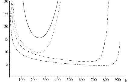
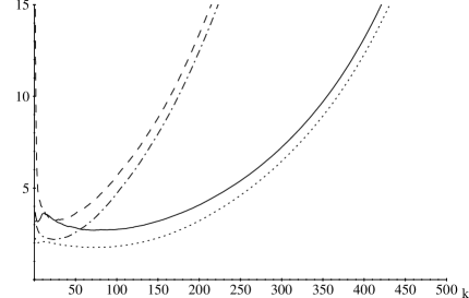
Figure 1: Simulated RMSE and $L_{1}$-error of the quantile estimator directly applied to the data (solid resp. dotted line) and of the quantile estimator based on the analysis of residuals (dashed resp. dash-dotted line) vs. number $k$ of order statistics for a linear $AR(1)$ time series; left plot: innovations according to Model a), right plot: Model b)

	Model a)		Model b)
	RMSE	$L_{1}$-error	RMSE	$L_{1}$-error
	bias / s.e.		bias / s.e.
direct estimation	15.4  (k=249)	9.7  (k=249)	2.7  (k=73)	1.8  (k=70)
	3.3 / 15.0		0.7 / 2.6
model based estimation	6.1  (k=662)	4.5  (k=765)	3.2   (k=25)	2.2 (k=23)
	-0.6 / 6.0		1.1 / 3.0

Table 1: Minimal errors, bias and standard errors of the quantile estimators in the (unperturbed linear) $AR(1)$ time series models

From these results, one gets the impression that, although the model-based approach does not yield more accurate estimators for all distributions of innovations, its overall performance is at least as good as the performance of the direct nonparametric approach. However, as we will see next, this interpretation is premature (and indeed quite dangerous) as the model-based estimator can be very sensitive to relatively small deviations to the model.

As an example, we consider a nonlinear $AR(1)$ time series, namely a stationary solution to the equation

$$X_{t}=\varphi_{1}X_{t-1}+\delta\mathrm{sgn}(X_{t-1})\log\big{(}\max(|X_{t-1}|,1)\big{)}+Z_{t}\qquad\text{with }\varphi=0.8,\,\delta=0.6.$$ (2.9)

Here the linear relationship between $X_{t}$ and $X_{t-1}$ is perturbed by an extra logarithmic term. Of course, one cannot expect that the relationship (2.8) holds in this nonlinear model. Hence, most likely, the model-based estimator will show an increased bias.

From Figure 2, which shows a typical scatterplot of $(X_{t-1},X_{t})$ for a time series according to model (2.9) with shifted double-sided Pareto innovations from Model b), it is apparent that, with the naked eye, such a time series can hardly be distinguished from a classical linear $AR(1)$ time series (with an increased autoregressive coefficient). Moreover, if one fits a linear $AR(1)$ model to such a time series of length $n=2000$, then the turning point test and the difference-sign test with nominal size 0.05 (see Brockwell and Davis (2002), p. 36 f.) detect dependence in the residuals with probability less than 0.06, i.e. these tests are not capable of detecting the model deviation. Also the Portmanteau test with nominal size 0.05 applied to the residuals has a maximal power of about 0.13, i.e. the rejection rate is less than 0.1 higher than the false alarm rate if the data comes from the corresponding $AR(1)$ model. (Note that the Portmanteau test should not be applied if the variance of the innovations is infinite; hence, strictly speaking, it is not suitable for Model a).) To sum up, it is almost impossible to distinguish a time series from model (2.9) from a linear $AR(1)$ time series.

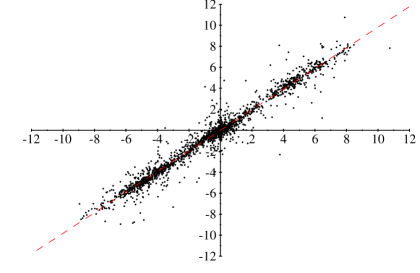
Figure 2: Scatterplot $(X_{t-1},X_{t})$ of a simulated nonlinear $AR(1)$ time series (2.9) of length $n=2000$ with innovations according to Model b); the dashed line indicates the fitted linear relationship with estimated autoregressive coefficient 0.982

Figure 3 shows the RMSE and $L_{1}$-errors of the quantile estimator obtained from the direct approach and the model-based approach when the time series are simulated according to (2.9), but erroneously a linear $AR(1)$ model is assumed. Table 2 gives the minimal errors in this case (analogously to Table 1). For both d.f.s of the innovations, the errors of the model-based quantile estimators are much larger in the nonlinear $AR(1)$ model than for the classical linear $AR(1)$ time series. To a large extent, the deterioration of the performance is caused by the large bias, but also the variance is much larger now even if the decrease of the optimal number of order statistics is taken into account. In sharp contrast, the direct quantile estimator, which does not rely on a specific time series model, is more precise for these nonlinear $AR(1)$ time series than for the linear ones. Consequently, if the innovations are drawn from Model a), then the minimal RMSE of the model-based quantile estimator is about 25% larger than the minimal RMSE of the direct quantile estimator, while for innovations according to Model b) the RMSE of the model-based estimator is more than 7 times larger than the RMSE of the nonparametric estimator!

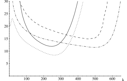
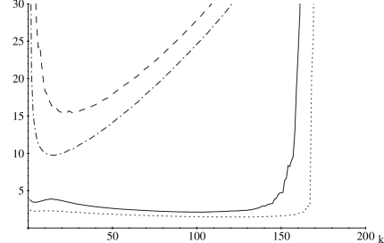
Figure 3: Simulated RMSE and $L_{1}$-error of the quantile estimator directly applied to the data (solid resp. dotted line) and of the quantile estimator based on the analysis of residuals (dashed resp. dash-dotted line) vs. number $k$ of order statistics for the nonlinear $AR(1)$ time series (2.9); left plot: innovations according to Model a), right plot: Model b)

	Model a)		Model b)
	RMSE	$L_{1}$-error	RMSE	$L_{1}$-error
	bias / s.e.		bias / s.e.
direct estimation	11.9   (k=247)	8.4  (k=260)	2.1   (k=99)	1.5   (k=122)
	-0.0 / 11.9		0.0 / 2.1
model based estimation	14.9   (k=462)	11.4   (k=498)	15.4  (k=22)	9.7  (k=16)
	9.2 / 11.7		9.5 / 12.1

Table 2: Minimal errors, bias and standard errors of the quantile estimators in the nonlinear $AR(1)$ time series (2.9)

Figure 4 demonstrates that the very poor performance of the quantile estimator which is based on the residual analysis is not due a few particularly wrong estimates but that indeed the estimator yields rather poor results with a high probability. In this plot, for innovations according to Model b), kernel estimates of the density of the direct (solid line) and the model-based quantile estimators (dashed line) are displayed for optimal values of $k$ (i.e., $k=99$ and $k=22$, respectively). While the mode of both densities is close to the true value (indicated by the vertical dotted line), the density of the model-based estimator is strongly skewed to the right and has a large spread. In contrast, the distribution of the nonparametric estimator is more symmetric and much more concentrated around the true value.

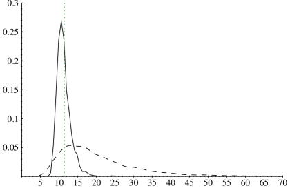
Figure 4: Estimated density of the direct quantile estimator (solid line) and the model-based estimator (dashed line) for time series according to (2.9) with innovations according to Model b); the true quantile is indicated by the vertical dotted line

To sum up, the example shows that the model-based approach to the estimation of extreme quantiles can give completely misleading estimates even if the deviation from the assumed linear time series model is moderate in the sense that it is very difficult to detect by means of statistical tests. Therefore, it seems advisable to use estimators only with utmost care which are based on an extreme value analysis of residuals obtained under parametric model assumptions about the dependence structure. In particular, it is not justified to consider them generally superior to the directly applied extreme value estimators.

3 Analysis of the extremal dependence structure: Is there a world behind the extremal index?

So far we have only considered estimators of the marginal tail behavior. For many applications, also the dependence between consecutive extreme values of the time series is of interest. For example, if $X_{t}$ denotes the negative return (loss) of some financial investment, it is important to assess the risk that all (or some of) the losses $X_{t},X_{t+1},\ldots,X_{t+m-1}$ in $m$ consecutive periods (or perhaps the total loss $\sum_{i=0}^{m-1}X_{t+i}$) are large.

In the analysis of the extreme value behavior of maxima $M_{n}:=\max_{1\leq t\leq n}X_{t}$ of $n$ consecutive observations the so-called extremal index plays a crucial role. Let $\tilde{X}_{t}$, $1\leq t\leq n$, denote an associated sequence of i.i.d. random variables with d.f. $F_{X}$. Assume that, for some normalizing constants $a_{n}>0$ and $b_{n}\in{\mathbb{R}}$,

$$\frac{\max_{1\leq t\leq n}\tilde{X}_{t}-b_{n}}{a_{n}}\;\longrightarrow\;G$$

weakly for some nondegenerate d.f. $G$. Leadbetter (1983) proved that then

$$\frac{M_{n}-b_{n}}{a_{n}}\;\longrightarrow\;G^{\theta}$$

for some $\theta\in[0,1]$ provided Leadbetter’s condition $D(u_{n})$

$$\forall\,m,n>0\;\exists\,\alpha_{n,m}\;\forall\,k,l>0,\,1\leq i_{1}<i_{2}<\ldots<i_{k}<i_{k}+m\leq j_{1}<j_{2}<\ldots<j_{l}\leq n:$$

$$\bigg{|}P\Big{\{}\max_{1\leq r\leq k}X_{i_{r}}\leq u_{n},\;\max_{1\leq s\leq l}X_{i_{s}}\leq u_{n}\Big{\}}-$$

$$\hskip 85.35826pt-P\Big{\{}\max_{1\leq r\leq k}X_{i_{r}}\leq u_{n}\Big{\}}\cdot P\Big{\{}\max_{1\leq s\leq l}X_{i_{s}}\leq u_{n}\Big{\}}\bigg{|}\leq\alpha_{n,m}$$

and $$\exists\,m_{n}=o(n):\quad\lim_{n\to\infty}\alpha_{n,m_{n}}=0$$

holds for all $u_{n}=a_{n}x+b_{n}$ with $x>G^{-1}(0)$, and the d.f. $P\{(M_{n}-b_{n})/a_{n}\leq x\}$ of the standardized maximum converges for some $x>G^{-1}(0)$. Hence, if the extremal index $\theta$ is strictly positive, the maximum converges to some nondegenerate limit distribution that is of the same type as the limit distribution in the case of independence.

Moreover, Hsing, Hüsler and Leadbetter (1988) proved that under weak additional assumptions (including the slightly stronger mixing condition $\Delta(u_{n})$) the point process $\sum_{t=1}^{n}{\varepsilon}_{t/n}1_{(a_{n}x+b_{n},\infty)}(X_{t})$ of standardized time points at which exceedances occur converges to a compound Poisson process. Then, typically, the extremal index $\theta$ equals the reciprocal value of its mean cluster size (although in general one only knows that $\theta$ is a lower bound for this value).

Since the asymptotic behavior of maxima of consecutive observations is completely determined by the extremal index and the tail behavior of $F_{X}$, the literature on the statistical analysis of the extremal dependence structure focusses on the estimation of $\theta$ and, to a lesser extent, the estimation of the cluster size distribution; see Hsing (1991, 1993), Smith and Weissman (1994), Weissman and Novak (1998), Ancona-Navarrete and Tawn (2000) and Ferro and Segers (2003), among others.

However, as the aforementioned example shows, in financial applications often other statistics of extreme values (than maxima) are of main interest, and the same holds true in other fields of applications where exceedances over high thresholds rather than block maxima are considered. We will demonstrate by a particular time series model that the extremal index and the cluster size distributions are often not sufficient to determine the distribution of statistics which arise in a natural way.

In the remainder of this section, we consider stationary solutions of stochastic recurrence equations of the type

$$X_{t}=A_{t}X_{t-1}+B_{t},\qquad t\in{\mathbb{Z}},$$ (3.10)

with $(A_{t},B_{t})$ denoting i.i.d. random vectors with values in $(0,\infty)^{2}$. For instance, a squared $ARCH(1)$ time series satisfies this relationship; further applications of this model were described by Vervaat (1979). Kesten (1973) proved that such a stationary solution exists if $A_{1}$ does not have a lattice distribution, the distribution of $B_{1}/(1-A_{1})$ is not degenerate, and if there exists $\kappa>0$ such that $EA_{1}^{\kappa}=1$, $E(A_{1}^{\kappa}\max(\log A_{1},0))<\infty$ and $EB_{1}^{\kappa}\in(0,\infty)$. Moreover, then $\bar{F}_{X}(x)\sim cx^{-\kappa}$ for some $c>0$ so that the standardized maxima of an accompanying i.i.d. sequence converge to a Fréchet distribution with extreme value index $\gamma=1/\kappa$.

De Haan et al. (1989) calculated the extremal index and the cluster size distribution of such a time series. Let $W_{j}=\prod_{i=1}^{j}A_{i}^{\kappa}$ (with the convention $W_{0}=1$). Note that $\log W_{j},j\geq 1,$ is a random walk with negative drift. Hence the sequence $W_{j},j\geq 1,$ tends to 0 and it is almost surely bounded. Let $U_{k}$ denote the $k$th largest value of this sequence. Then the extremal index $\theta$ and the probability $\pi_{k}$ that a cluster of the limiting compound Poisson point process has size $k$ are given by

$$\theta = \int_{0}^{1}P\big{\{}U_{1}=\max_{j\geq 1}W_{j}\leq t\big{\}}\,dt\;=\;1-E\min(U_{1},1),$$

$$\pi_{k} = \frac{\theta_{k}-\theta_{k+1}}{\theta}\qquad\text{with}$$ (3.11)

$$\theta_{k} = \int_{0}^{1}P\Big{\{}\sum_{j=1}^{\infty}1_{(t,\infty)}(W_{j})=k-1\Big{\}}\,dt\;=\;E\big{(}\min(U_{k-1},1)-\min(U_{k},1)\big{)}.$$

Hence the extremal index is determined by the distribution of the maximum of the geometric random walk $W_{j},j\geq 1$, and the probability that a cluster of exceedances has size $k$ is determined by the distributions of the $k$ largest “order statistics” of this sequence.

More recently, Gomes et al. (2004) (see also Gomes et al. (2006)) analyzed the joint asymptotics of $k$ consecutive observations of the stationary solution of the recurrence equation (3.10). More precisely, they proved that there exists a sequence $a_{n}>0$ such that

$$\lim_{n\to\infty}nP\big{\{}X_{j}>a_{n}x_{j}\;\text{ for all }1\leq j\leq k\big{\}} = E\min_{0\leq j\leq k-1}(x_{j}^{-\kappa}W_{j}),$$

$$\lim_{n\to\infty}nP\big{\{}X_{j}>a_{n}x_{j}\;\text{ for some }1\leq j\leq k\big{\}} = E\max_{0\leq j\leq k-1}(x_{j}^{-\kappa}W_{j}),$$

for all $x_{j}>0$. Obviously, the limits on the right hand sides cannot be expressed in terms of the extremal index $\theta$ and the cluster size distribution $\pi_{k},k\geq 1,$ for all $x_{j}>0$. However, this will not even be possible in the special case that all $x_{j}$ are equal to some $x$, say, so that

$$\lim_{n\to\infty}nP\big{\{}X_{j}>a_{n}x\;\text{ for all }1\leq j\leq k\big{\}} = x^{-\kappa}E\min_{0\leq j\leq k-1}W_{j}$$

$$= x^{-\kappa}\int_{0}^{1}P\big{\{}\min_{0\leq j\leq k-1}W_{j}>t\big{\}}\,dt,$$

$$\lim_{n\to\infty}nP\big{\{}X_{j}>a_{n}x\;\text{ for some }1\leq j\leq k\big{\}} = x^{-\kappa}E\max_{0\leq j\leq k-1}W_{j}$$

$$= x^{-\kappa}\int_{0}^{\infty}P\big{\{}\max_{0\leq j\leq k-1}W_{j}>t\big{\}}\,dt,$$

because the right hand sides depend on the distribution of the minimum and the maximum of a finite segment of the sequence $W_{j},j\geq 1,$ instead of the distribution of the order statistics of the whole sequence.

The asymptotic variance of the Hill estimator discussed in Section 2 is another example of a parameter which arises naturally in statistical applications and cannot be determined from the extremal index and the cluster size distribution. Drees (2000) showed that the Hill estimator based on the $k$ largest observations of a stationary solution of the recurrence equation (3.10) is asymptotically normal with variance

$$\kappa^{-2}\Big{(}1+2\sum_{j=1}^{\infty}\int_{0}^{1}P\{W_{j}>t\}\,dt\Big{)},$$

provided that $k$ tends to $\infty$ not too fast. (An analogous result holds true for the maximum likelihood estimator of the extreme value index, which is asymptotically normal with a similar variance with factor $(1+1/\kappa)^{2}$ instead of $\kappa^{-2}$.) Here, the parameter is determined by all marginal distributions of the geometric random walk $W_{j}$, $j\geq 1$.

These examples demonstrate that in many applications the extremal index (and often also the cluster size distribution) does not give the information one is actually interested in. Thus there is clearly a need to put the statistical analysis of the extremal dependence on a broader basis such that also parameters can be treated which describe aspects of the dependence structure different from the size of clusters of exceedances.

An interesting point of departure may be the concept of cluster functionals introduced by Yun (2000) and developed further by Segers (2003). Roughly speaking, these are functionals which depend only on all shortest vectors of observations containing exceedances over a given high threshold. An asymptotic theory on estimators of functionals of that type would be a significant step forward towards a general approach to analyze the extremal dependence structure of stationary time series.

4 Conclusions

In Section 2 we compared the direct approach to the marginal tail analysis, advocated by Rootzén, Leadbetter and de Haan (1990), among others, with a model-based approach where the tail of the residuals is analyzed. It was pointed out that the perception that the latter approach is more efficient when the model assumptions are correct is not generally justified. Moreover, it was shown that the model-based estimators can be extremely sensitive to moderate deviations from the models, which are difficult to detect by statistical means. Hence, in most applications, the direct nonparametric analysis, that has proved powerful in the classical i.i.d. setting in several papers by Laurens de Haan and many others, seems also preferable for the tail analysis of serially dependent data.

It is worth mentioning that usually the model-based approach is even more problematic if a nonlinear time series model is assumed. For example, as we have seen in Section 3, the marginal tail behavior of a stationary solution to the stochastic recurrence equation (3.10) does not only depend on the tail of the “innovations” $A_{t}$ (and $B_{t}$), but on their whole distribution, since the extreme value index $\gamma=1/\kappa$ is determined by the relationship $EA_{1}^{\kappa}=1$. So, in a parametric submodel, it will not be sufficient to analyze the tail behavior of suitably defined residuals, but one has to estimate this expectation, that depends on the center of the distribution of the innovations and, in addition, is sensitive to deviations in the tail. Hence, to obtain a reliable estimate, usually one has to combine some nonparametric estimate for the central region with an extreme value estimator for the tail of the distribution of the innovations, which makes the whole method cumbersome.

While in the marginal tail analysis sometimes too restrictive model assumptions are used, the inference on the extremal dependence structure is often too focussed on the extremal index (which is then estimated in quite general time series models). The nonlinear time series (3.10) is a nice example in which parameters arise in a natural way which cannot be expressed in terms of the extremal index or the cluster size distribution. This observation calls for more general estimators of the extremal dependence structure. Unfortunately, even from the most optimistic point of view, such a general theory has just started to emerge and many challenging problems still wait for a solution.

Acknowledgement: The author is grateful to Jürg Hüsler and Peng Liang for pointing out the reference Barbe and McCormick (2004).

References

Ancona-Navarrete, M.A., and Tawn, J.A. (2000). A comparison of methods for estimating the extremal index. Extremes 3, 5–38.

Barbe, Ph., McCormick, W.P. (2004). Tail calculus with remainder, applications to tail expansions for infinite order moving averages, randomly stopped sums, and related topics. Extremes 7, 337–365.

Brockwell, P.J., and Davis, R.A. (2002). Introduction to Time Series and Forecasting (2nd ed). Springer.

Datta, S., and McCormick, W.P. (1998). Inference for the tail parameters of a linear process with heavy tail innovations. Ann. Inst. Statist. Math. 50, 337–359.

Davis, R.A., and Resnick, S.I. (1985). Limit theory for moving averages of random variables with regularly varying tail probabilities. Ann. Probab. 13, 179–195.

Dekkers, A.L.M., and de Haan, L. (1989). On the estimation of the extreme-value index and large quantile estimation. Ann. Statist. 17, 1795–1832.

Drees, H. (2000). Weighted approximations of tail processes for $\beta$–mixing random variables. Ann. Appl. Probab. 10, 1274–1301.

Drees, H. (2002). Tail empirical processes under mixing conditions. In: H.G. Dehling, T. Mikosch und M. Sørensen (eds.), Empirical Process Techniques for Dependent Data, 325–342, Birkhäuser, Boston.

Drees, H. (2003). Extreme quantile estimation for dependent data with applications to finance. Bernoulli 9, 617–657.

Ferro, C.A.T., and Segers, J. (2003). Inference for clusters of extreme values. J. Roy. Statist. Soc. B, 65, 545–556.

Geluk, J.L., Peng, L., and de Vries, C.G. (2000). Convolutions of heavy-tailed random variables and applications to portfolio diversification and ${\rm MA}(1)$ time series. Adv. Appl. Probab. 32 , 1011–1026.

Geluk, J. L., and Peng, L. (2000). An adaptive optimal estimate of the tail index for ${\rm MA}(1)$ time series. Statist. Probab. Lett. 46, 217–227.

Gomes, M.I., de Haan, L., and Pestana, D. (2004). Joint exceedances of the ARCH process. J. Appl. Probab. 41, 919–926.

Gomes, M.I., de Haan, L., and Pestana, D. (2006). Correction to: Joint exceedances of the ARCH process. J. Appl. Probab. 43, 1206.

de Haan, L. (1990). Fighting the arch-enemy with mathematics. Statist. Neerlandica 44, 45–68.

de Haan, L., Resnick, S.I., Rootzén, H., and de Vries, C. (1989). Extremal behaviour of solutions to a stochastic difference equation with applications to ARCH-processes. Stoch. Proc.  Appl. 32, 213–224.

de Haan, L., and de Ronde, J. (1998). Sea and wind: multivariate extremes at work. Extremes 1, 7–45.

de Haan, L., and Stadtmüller, U. (1996). Generalized regular variation of second order. J. Aust. Math. Soc. A 61, 381–395.

Hsing, T. (1991). On tail estimation using dependent data. Ann. Statist. 19, 1547–1569.

Hsing, T. (1993). Extremal index estimation for a weakly dependent stationary sequence. Ann. Statist. 21, 2043–2071.

Hsing, T., Hüsler, J., and Leadbetter, M.R. (1988). On the exceedance point process for a stationary sequence. Probab. Theory Relat. Fields 78, 97–112.

Kesten, H. (1973). Random difference equations and renewal theory for products of random matrices. Acta Math. 131, 207–248.

Leadbetter, M.R. (1983). Extremes and local dependence in stationary sequences. Probab. Theory Relat. Fields 65, 291–306.

Leadbetter, M.R. (1995). On high level exceedance modeling and tail inference. J. Statist. Plann. Inference 45, 247–260.

Leadbetter, M.R., and Rootzén, H. (1993). On central limit theory for families of strongly mixing additive random functions. In: Stochastic processes: a festschrift in honour of Gopinath Kallianpur (S. Cambanis et al., eds.), 211–223. Springer.

Ledford, A.W., and Tawn, J.A. (2003). Diagnostics for dependence within time series extremes. J. Royal Statist. Soc. B 65, 521- 543.

Ling, S., and Peng, L. (2004). Hill’s estimator for the tail index of an ARMA model. J. Statist. Plann. Inference 123, 279–293.

Mikosch, T., and Samorodnitsky, G. (2000). The supremum of a negative drift random walk with dependent heavy-tailed steps. Ann. Appl. Probab. 10, 1025–1064.

Novak, S.Y. (2002). Inference on heavy tails from dependent data. Siberian Adv. Math. 12, 73–96.

Pereira, T.T. (1994). Second order behaviour of domains of attraction and the bias of generalized Pickands’ estimator. In: Extreme Value Theory and Applications III (J. Galambos, J. Lechner and E. Simiu, eds.), 165–177. NIST special publication 866.

Resnick, S., and Stǎricǎ, C. (1997). Asymptotic behavior of Hill’s estimator for autoregressive data. Comm. Statist. Stochastic Models 13, 703–721.

Rootzén, H. (1995). The tail empirical process for stationary sequences. Unpublished manuscript, Chalmers University Gothenburg.

Rootzén, H. (2006). Weak convergence of the tail empirical process for stationary sequences. Submitted.

Rootzén, H., Leadbetter, M.R., and de Haan, L. (1990). Tail and quantile estimators for strongly mixing stationary processes. Report, Department of Statistics, University of North Carolina.

Rootzén, H., Leadbetter, M.R., and de Haan, L. (1998). On the distribution of tail array sums for strongly mixing stationary sequences. Ann. Appl. Probab. 8, 868–885.

Segers, J. (2003). Functionals of clusters of extremes. Adv. Appl. Probab. 35, 1028–1045.

Smith, R.L., and Weissman, I. (1994). Estimating the extremal index. J. Roy. Statist. Soc. B 56, 515–528.

Vervaat, W. (1979). On a stochastic difference equation and a representation of non-negative infinitely divisible random variables. Adv. Appl. Probab. 11, 750–783.

Weissman, I., and Novak, S.Yu. (1998). On blocks and runs estimators of the extremal index. J. Statist. Plann. Inference 66, 281–288.

Yun, S. (2000). The distribution of cluster functionals of extreme events in a $d$th-order Markov chain. J. Appl. Probab. 37, 29–44.