Ultra-high-time Resolution Observations of Radio Bursts on AD Leonis

Abstract

We report observations of a radio burst that occurred on the flare star AD Leonis over a frequency range of 1120-1620 MHz ($\lambda\approx$18–27 cm). These observations, made by the 305 m telescope of the Arecibo Observatory, are unique in providing the highest time resolution (1 ms) and broadest spectral coverage ($\Delta\nu/\nu=0.36$) of a stellar radio burst yet obtained. The burst was observed on 2005 April 9. It produced a peak flux density of $\sim 500$ mJy and it was essentially 100% right-circularly polarized. The dynamic spectrum shows a rich variety of structure: patchy emission, diffuse bands, and narrowband, fast-drift striae. Focusing our attention on the fast-drift striae, we consider the possible role of dispersion and find that it requires rather special conditions in the source to be a significant factor. We suggest that the emission may be due to the cyclotron maser instability, a mechanism known to occur in planetary magnetospheres. We briefly explore possible implications of this possibility.

1 Introduction

The use of radio dynamic spectra has played a central role in identifying and clarifying the physical mechanisms at work in the solar corona (see McLean & Labrum, 1985, for reviews). The application of similar techniques to active stars has long been an important goal, but it has been hampered by limitations in available instrumentation. Past studies of radio emission from M dwarf flare stars led to the discovery of extreme stellar radio bursts, characterized by close to 100% circularly polarized emission with brightness temperatures in excess of 10¹⁴K and durations less than a few tens of milliseconds (Güdel et al., 1989; Bastian et al., 1990). However, these spectroscopic investigations of the coherent radio bursts on flare stars have typically been limited by relatively long integration times (Bastian & Bookbinder, 1987; Güdel et al., 1989) and/or limited frequency bandwidth ratios $\Delta\nu/\nu$ (usually just a few percent; e.g., Bastian et al., 1990; Abada-Simon et al., 1997). The necessary combination of high time resolution and a large frequency bandwidth ratio has only been available infrequently (Stepanov et al., 2001; Zaitsev et al., 2004), precluding measurements of key parameters such as the intrinsic frequency bandwidth or frequency drift rate of the radio bursts, making the interpretation of these puzzling events difficult. It is only with the recent advent of radio spectrometers capable of supporting both a large bandwidth ratio and high time resolution simultaneously that progress in understanding the physics of radio bursts in the coronas of other stars becomes possible.

AD Leonis, a young disk star at a distance of 4.9 pc from the Sun, is one of the most active flare stars known, producing intense, quasi-steady chromospheric and coronal emissions (Hawley et al., 2003; Hünsch et al., 1999; Jackson et al., 1989) seen at UV, X-ray, and radio wavelengths. The star is also highly variable, producing flares from radio to X-ray wavelengths (e.g., Bastian et al., 1990; Hawley & Pettersen, 1991; Hawley et al., 2003, 1995; Favata et al., 2000). Its propensity for frequent and extreme radio bursts (with intensities peaking at $>$ 500 times the quiescent radio luminosity of 5.5$\times$10¹³ erg s^-1 Hz^-1; Jackson et al., 1989) makes it a frequent target for radio investigations of stellar flares. In a previous paper (Osten & Bastian, 2006, hereafter, Paper I) we described the initiation of a pilot program to observe active M dwarfs with the Arecibo Observatory’s Wideband Arecibo Pulsar Processor (WAPP), and first results from that program. Here we describe the next phase, which increased the time resolution by a factor of 10 to 1 ms.

2 Observations

We observed AD Leo with the 305 m telescope at Arecibo Observatory on each of four days from 2005 April 8–11, during which time approximately $4\times 4$ hours of data were collected. The observations were made using the “L-band wide” dual-linear feed and receiver (1100-1700 MHz) with the Wideband Arecibo Pulsar Processor (WAPP) backend. The WAPP was selected because it provides the means of observing a large instantaneous bandwidth with excellent spectral and temporal resolution. The WAPP provides four data channels, each of 100 MHz bandwidth. These were deployed across the L-band wide receiver as follows: 1120–1220 MHz, 1320–1420 MHz, 1420–1520 MHz, and 1520–1620 MHz. A gap was deliberately left between 1220–1320 MHz to avoid the strong radio frequency interference (RFI) present in this frequency range. Nevertheless, the effects of other sources of RFI could not be entirely avoided in the frequency bands observed. We employed a data acquisition mode where data were sampled with a time resolution of 1 ms; 128 spectral channels were sampled across each 100 MHz channel, yielding a spectral resolution of 0.78 MHz. All four correlation products were recorded between the native-linear X and Y feed elements (XX, YY, XY, YX) with three-level sampling. Our observing strategy was to observe the target, AD Leo, for 10 minute scans, and then to inject a correlated calibration signal to determine the amplitude and phase calibration of the two polarization channels. A standard calibrator source, B1040+123, was also observed prior to each of the four observing runs.

The beam size using the L-band wide receiver at 1.4 GHz is $\approx 3.1\times$3.5 arcminutes in azimuth and zenith angle. Interferometric measurements of AD Leo’s 1.4 GHz flux density during periods of apparent quiescence are $\approx 2$ mJy (Jackson et al., 1989), well below the confusion limit of Arecibo at the observed frequencies ($\approx$ 16–38 mJy from 1120 MHz to 1620 MHz). Although there is a bright background radio source located $\approx$ 2.3 arcminutes away from AD Leo (Seiradakis et al., 1995) and therefore within the primary beam, we utilized a “time-switching” scheme to difference times of burst activity (“on”) and the quiescent state plus background (“off”). The source of radio bursts has been confirmed as AD Leo in past years using a variety of techniques: interferometric observations by the VLA (Bastian & Bookbinder, 1987), or the characteristic frequency modulation of sources in the main beam of the line feeds formerly used at Arecibo (Bastian et al., 1990). Our calibration approach enabled us to estimate the antenna temperature and flux density through the use of gain curves as a function of azimuth and zenith angle. We determined the rms uncertainty in regions of the dynamic spectrum where no bursting behavior was evident, estimating the 1 $\sigma$ noise uncertainty for various time resolutions to be $(1.6-2.2)/\sqrt{\tau}$ mJy/channel, where $\tau$ is the integration time in seconds.

3 Data Analysis and Results

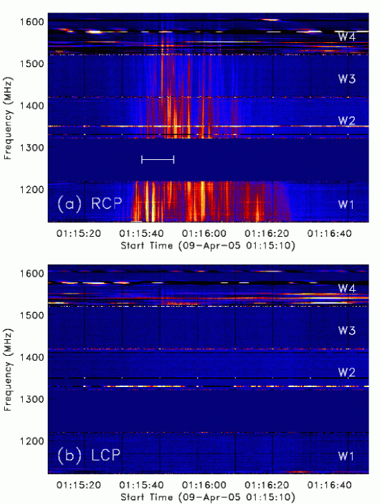
Figure 1: Overview of the radio burst observed on AD Leo. a) Right-circularly polarized emission. b) Left-circularly polarized emission. The data have been averaged to 100 ms time resolution. The four WAPP data channels are labeled W1, W2, W3, and W4. The frequency range of 1220-1320 MHz was deliberately avoided due to the presence of strong RFI. Nevertheless, bright and dark horizontal bands and faint periodic vertical bands indicate the presence of RFI that could not be avoided. A detail of the 10 s time interval indicated by the horizontal bar is shown in Fig. 2.

A spectacular radio burst occurred on 2005 April 9 at approximately 01:15:40 UT. An overview of the event is shown in Fig. 1 with a time resolution of 100 ms. Note the data gap between 1220-1320 MHz and horizontal features due to RFI. The radio burst is essentially 100% right-circularly polarized (RCP; Fig. 1a). The emission is bounded in frequency from above, the upper limit ranging from $\approx 1200-1600$ MHz. The low frequency limit of the emission is unknown because of a lower limit imposed by the spectrometer. The emission presumably extends well below 1120 MHz.

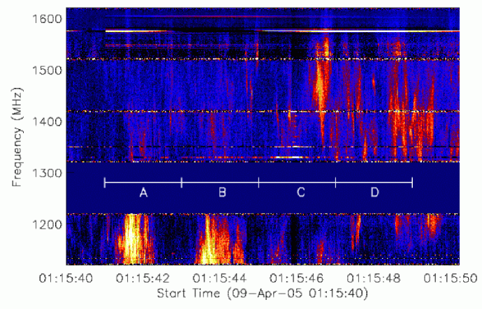
Figure 2: A detail of the RCP spectrum indicated by the bar in Fig. 1a at a time resolution of 10 ms. Further details of the spectrum for consecutive 2 s time intervals labeled A, B, C, and D are shown in Fig. 3.

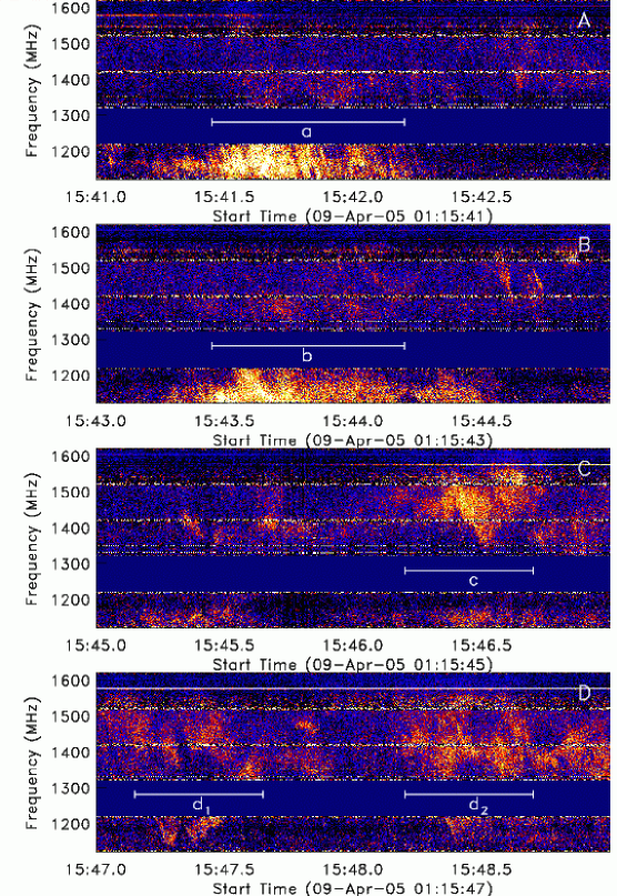
Figure 3: Details of the RCP spectrum shown in Fig. 2. Each panel A-D shows 2 s of data with the full time resolution of 1 ms.

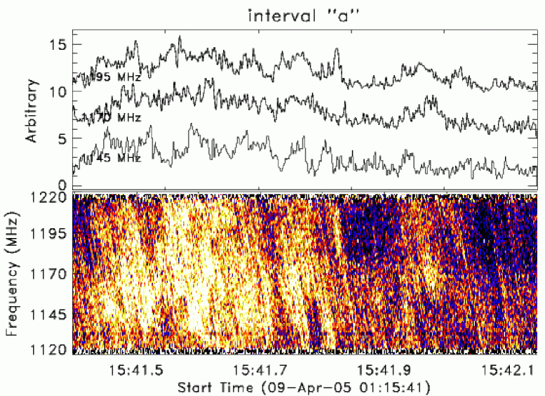
Figure 4: Detail of the RCP spectrum indicated by the bar in Fig. 3, panel A, labeled “a”. The frequency range shown is 1120-1220 MHz, the time interval is 0.75 s, and the time resolution is 1 ms. The upper panel shows the time variation of flux density at the frequencies indicated. Note the fast-drift striations.

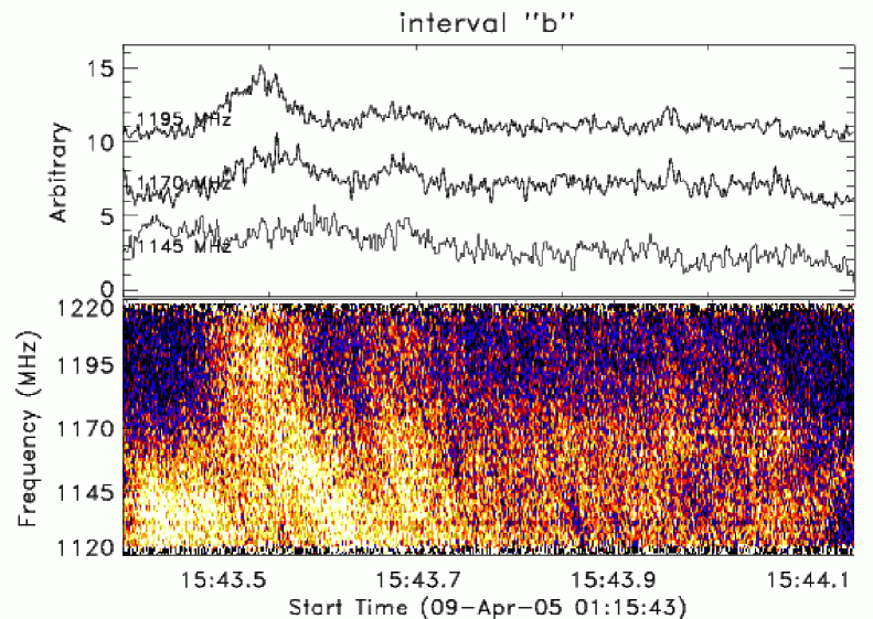
Figure 5: Detail of the RCP spectrum as indicated by the bar in Fig. 3, panel B, labeled “b”. The frequency range shown is 1120-1220 MHz, the time interval is 0.75 s, and the time resolution is 1 ms. Here the emission is relatively diffuse.

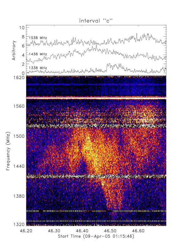
Figure 6: Detail of the RCP spectrum as indicated by the bar in Fig. 3, panel C, labeled “c”. The frequency range shown is 1320-1620 MHz, the time interval is 0.5 s, and the time resolution is 1 ms. The emission is again relatively diffuse, with considerable variation in bandwidth.

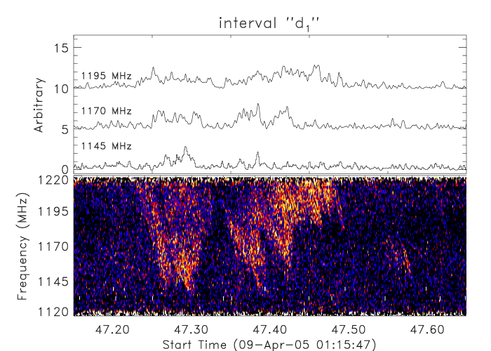
Figure 7: Detail of the RCP spectrum as indicated by the bar in Fig. 3, panel D, labeled “d₁”. The frequency range shown is 1120-1220 MHz, the time interval is 0.5 s, and the time resolution is 1 ms.

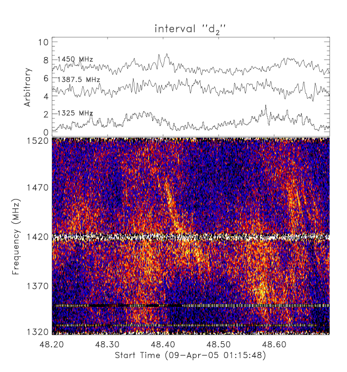
Figure 8: Detail of the RCP spectrum as indicated by the bar in Fig. 3, panel D, labeled “d₂”. The frequency range shown is 1320-1520 MHz, the time interval is 0.5 s, and the time resolution is 1 ms.

While the burst was only $\approx 45$ s in duration, it was observed with a time resolution of 1 ms. In the following, we confine our attention to only a small part of the data which nevertheless shows a rich variety of spectral signatures. The horizontal bar shown in Fig. 1, spanning the most intense RCP emission, indicates the 10 s interval shown in Fig. 2 with a time resolution of 10 ms. The four consecutive 2 s time intervals labeled (A-D) in Fig. 2 are, in turn, shown with 1 ms time resolution in Fig. 3. It is readily apparent that the radio emission is spectrally and temporally complex. Details of time intervals a–d₂ are shown in Figs. 4-8 over restricted bands but with 1 ms time resolution.

Fig. 4 is of particular interest. It shows a 0.75 s interval of the spectrum corresponding to time interval “a” in Fig. 3, panel A. The frequency interval shown is 1120-1220 MHz. An intense series of striae are visible, drifting from high to low frequencies with time. It is difficult to determine whether an underlying diffuse component exists or whether the striae recur so fast that they overlap and merge. It is therefore difficult to isolate and characterize the bandwidths and durations of single stria. Nevertheless, their durations have been constrained in aggregate as follows: first, the spectrum was smoothed in time channel by channel using a 50 ms running mean. Second, the smoothed spectrum was subtracted from the observed spectrum yielding a residual spectrum containing the rapidly varying striae. Third, to improve the signal to noise ratio, the residual spectrum was then “corrected” for the frequency drift of the striae by progressively shifting each channel in time to yield vertical striae. Note that if the drift rate were due to group delay, this operation would be referred to as de-dispersion; however, see §4.1. It is found that a range of drift rates is present in the striae, corresponding to delays of 43-48 ms per 100 MHz. The mean delay is 45 ms per 100 MHz. Therefore the mean drift rate is -2.2 GHz s^-1 with a range of -2.33 to -2.08 GHz s^-1 observed. Finally, the drift-corrected, residual spectrum was frequency-averaged over the central seventy (RFI-free) channels. All striae with an SNR$>4$ were accumulated, 32 in all. These have a mean FWHM duration of $\delta t\approx 2$ ms. A limit on the intrinsic source size $d$ follows by noting that $d<c\ \delta t\approx 600$ km. Coupled with the frequency drift rate of the striae, the mean duration implies a mean instantaneous bandwidth of 4.4 MHz, or $\Delta\nu/\nu\lesssim 0.5\%$. The recurrence rate of the striae is $>40$ s^-1 in this example.

Turning to other examples, Fig. 5 also shows 0.75 s of data (interval “b” in Fig. 3, panel B) from 1120-1220 MHz. The emission at this time, only 2 s after interval “a”, is far more diffuse than that shown in Fig. 4 although fast-drift structure is still visible. Fig. 6 shows 0.5 s of data (interval “c” in Fig. 3, panel C). Here, a frequency range of 1320-1620 MHz is shown. The emission is relatively diffuse; no striae are obviously present. The emission is frequency-bounded from above and below throughout the interval. The instantaneous frequency bandwidth varies from $\sim 20-180$ MHz ($\Delta\nu/\nu\sim 1.4-12.5\%$). Fig. 7 also shows a 0.5 s interval and a frequency range of 1120-1220 MHz (interval “d₁” in Fig. 3, panel D). This interval is striking in the abrupt onset and cessation of each patch of emission, and the crisply defined lower boundary to the frequency of emission. At least two patches are resolved in frequency, near 01:15:47.37 and 01:15:47.56 UT. These have bandwidths of 25 and $\sim 15$ MHz ($\Delta\nu/\nu\sim 1.3$ and $2.2\%$, respectively), the latter patch showing signs of band-limited striae. The other patches may likewise be composed of overlapping striae drifting from high to low frequency in the same sense as displayed in interval “a”. The upper frequency boundary is not known for the other patches because of the presence of the data gap between 1220-1320 MHz, but it is less than 1320 MHz. Finally, Fig. 8 again shows 0.5 s of data, but from 1320-1520 MHz, corresponding to the interval “d₂” in Fig. 3, panel D. Here, the emission is patchy and diffuse with some striae superposed, again with the same sense of drift as noted in prior intervals. Apparent frequency bandwidths range from $\sim 5$ MHz to $\gtrsim 200$ MHz ($\Delta\nu/\nu\sim 0.5-14\%$).

While these observations exploited the largest frequency-bandwidth ratio currently available (36%), the bandwidth is still insufficient to detect possible low-order harmonics of the emission because the ratio of the highest to the lowest frequency sampled is only 1.45:1. While higher harmonic ratios could in principle be detected – e.g., 4:3 – there is no evidence for such harmonic relations in the data. Therefore, no constraints on the emission mechanism are possible on the basis of harmonic structure.

To summarize, a variety of spectral structures – fast-drift striae, discrete patches, and diffuse emission – are seen in the few seconds of data presented here. The striae show a remarkably uniform drift rate of $\approx-2.2$ GHz s^-1. The durations of the striae, typically $\sim$2 ms, imply dynamical source sizes $\approx$0.2% of the stellar radius. The spectral features are resolved in frequency, showing bandwidths ranging from $\lesssim\!0.5\%$ to as much as 14%. Where drifting structures appear to be present, the sense of the drift is the same – the emission starts at high frequencies and proceeds to lower frequencies. The signatures appear only in RCP emission, indicating a high degree of circular polarization.

4 Discussion

In this section we focus our attention the striae shown in Fig. 4, the reason being that their properties – flux density, drift rate, mean duration, and mean bandwidth – are well constrained. We first consider whether the observed spectral features – notably the rapid frequency drift with time – could result from dispersion of the signal in the plasma due to group delay. We also consider propagation effects such as scintillation. We conclude that it is unlikely that propagation effects play a significant role. We then consider the relevant emission mechanism. We argue that, in contrast to the fast drift bursts presented in Paper I, the striae burst in the present case are unlikely the result of plasma radiation from electron beams and suggest that they may be due to the action of the cyclotron maser instability (CMI). We comment on the other burst phenomena at the end of the section.

4.1 Propagation Effects

As a radio wave traverses a plasma medium, it propagates at the group velocity $v_{g}=\mu c$, where $\mu=\sqrt{1-\nu_{pe}^{2}/\nu^{2}}$ is the refractive index and $\nu_{pe}^{2}=e^{2}n_{e}/\pi m_{e}$ is the electron plasma frequency, where $n_{e}$ is the electron number density in the plasma medium, $e$ is the electron charge, and $m_{e}$ is the electron mass. If a radio signal emitted at a frequency $\nu$ is received at a distance $d$ from the source, the delay in reception relative to a signal traversing the same distance in vacuo is

$$\Delta t={1\over c}\int_{0}^{d}({1\over\mu}-1)dr$$ (1)

We first consider the stellar corona and assume that the variation in electron number density can be described by a barometric model: $n_{e}(r)=n_{\circ}\exp(-r/\lambda_{n})$, where $\lambda_{n}$ is the number density scale height. If we assume that the observed emission is fundamental plasma radiation emitted at $r=R$, so that $\nu=\nu_{pe}(R)$, then the group delay equation can be recast (Wild et al., 1959), integrating from the location of the source emission to $\infty$, as

$$\Delta t={{2\lambda_{n}}\over c}\int_{0}^{1}{{d\mu}\over{1+\mu}}={{2\lambda_{n}\log 2}\over{c}}.$$ (2)

Under these circumstances the delay is frequency independent and an observed frequency drift can be attributed to source motion (Paper I).

On the other hand, if the emission occurs at frequencies well above the local plasma frequency ($\nu\gg\nu_{pe}$), then $1/\mu\approx 1+\nu_{pe}^{2}/2\nu^{2}$ and the relative delay between two frequencies can be written as

$$\Delta t={1\over c}\int_{R}^{\infty}\Bigl{[}{1\over{\mu(\nu_{1})}}-{1\over{\mu(\nu_{2})}}\Bigr{]}dr={{e^{2}}\over{2\pi m_{e}c}}\Bigl{[}{1\over{\nu_{1}^{2}}}-{1\over{\nu_{2}^{2}}}\Bigr{]}\int_{R}^{\infty}n_{e}(r)dr$$ (3)

where the integral quantity is commonly referred to as the dispersion measure. Supposing the source is intrinsically broadband and is located at least $3\lambda$ above the plasma level where $n=n_{\circ}\approx 1.7\times 10^{10}$ cm^-3, corresponding to a plasma frequency of 1170 MHz, $\Delta t<1.3\times 10^{-13}\lambda_{n}$ s. Taking $\lambda_{n}\sim 10^{10}$ cm, $\Delta t<1.3$ ms across the 100 MHz bandwidth, far less than the 45 ms observed in the striae described above. It is also worth considering the additional delay introduced by the interstellar medium. With a mean density of 0.1 cm^-3 (Cox & Reynolds, 1987) and a distance to AD Leo of 4.9 pc, we find that the incremental delay resulting from propagation through the ISM is only 0.25 ms across the 100 MHz band.

In fact, rather special conditions are required to account for the observed frequency drift in terms of impulsive broadband signals and group delay. The relative delay between two frequencies $\nu_{1}$ and $\nu_{2}$ within a source at a height $r$ is

$$\Delta t={{2\lambda_{n}}\over c}\int_{\mu_{1}(r)}^{\mu_{2}(r)}{{d\mu}\over{1+\mu}}={{2\lambda_{n}}\over{c}}\log{{1+\mu_{2}(r)}\over{1+\mu_{1}(r)}}.$$ (4)

where $\mu_{1,2}$ is the refractive index at $r$ for frequencies $\nu_{1,2}$. We find that the observed delay of 45 ms between 1120–1220 MHz can occur if the mean frequency of the band is $\approx 20\%$ above the plasma frequency $\nu_{pe}\approx 0.97$ GHz, where $\mu\sim 0.55$.

For completeness we mention that the presence of a magnetic field renders a plasma birefringent and radiation at a fixed frequency shows a differential delay between the ordinary and extraordinary modes, corresponding to a delay between RCP and LCP emissions. At frequencies where $\nu\gg\nu_{pe}$ and $\nu_{Be}$, the differential group delay between RCP and LCP over a path from the region of source emission to observation is (Benz & Pianezzi, 1997; Fleishman et al., 2002a, b)

$$\Delta t=\int\Bigl{[}\frac{1}{v_{x}}-\frac{1}{v_{o}}\Bigr{]}dr={{2\lambda_{n}}\over c}\ {{\nu_{pe}^{2}\nu_{Be}\cos\theta}\over{\nu^{3}}}$$ (5)

where $\nu_{Be}=eB/2\pi m_{e}c$ is the electron gyrofrequency and $\theta$ is the angle between the magnetic field and the line of sight. For the observations under consideration, the emission is essentially 100% RCP, discrete LCP features being indistinguishable from background. Hence, any differential delay between RCP and LCP is unmeasurable. Future observations of moderately polarized bursts with sufficient time resolution and frequency coverage may be able to exploit this technique.

We now briefly consider additional propagation effects that may influence the observed dynamic spectra. Turbulent interstellar plasma can produce scattering of radio waves propagating from point-like sources; for objects with high enough transverse velocity and/or long path length through the scattering medium, amplitude modulations, pulse broadening, and frequency smearing can occur. The slow amplitude variations of pulsars, maser sources, and compact cores of active galatic nuclei among other sources, have been identified as refractive interstellar scintillations (RISS) (see discussion in Rickett, 1990). Diffractive interstellar scintillation (DISS) occurs in the limit of strong scattering from small-scale irregularities in interstellar plasma, and corresponds to deep modulations in time and frequency. Dynamic spectra of pulsars reveal bands drifting in frequency and time, and criss-cross and periodic bands of emission, which qualitatively resemble some of the features seen in AD Leo’s dynamic spectrum; these features have been explained qualitatively by refractive steering of a diffractive interstellar scintillation pattern (Rickett, 1990). Could the observed spectral structure be due to scintillation as a result of propagation through the stellar corona and/or the ISM? Sources must be compact for either phenomenon (RISS or DISS) to occur. The small intrinsic source size implied by the extremely short durations of the observed emissions ($d<600$ km) suggests an angular size $\theta\sim d/D\lesssim\!1\mu$as. RISS corresponds to relatively (temporally) slowly varying intensities, and also should not change polarization variations (Rickett, 1990), thus inconsistent with the emission properties described earlier. DISS is usually seen in two-dimensional dynamic spectra; analysis of the two-dimensional Fourier transform of dynamic spectra reveals discrete structures which are typically explained as interference between two or more scattered images. Scintillation arcs due to DISS in pulsar dynamic spectra are a broadband phenomenon, having been observed over a factor of $\sim$5 in frequency (Hill et al., 2003). Pulse broadening due to multi-path scattering in the ISM can be estimated using equation (6) in Cordes & McLaughlin (2003) and Cordes & Lazio (2001) which, for a dispersion measure of 0.5 pc cm^-3, is $\sim$10^-10 s and therefore negligible. The scintillation bandwidth is inversely related to the pulse broadening time, which can be estimated as $\Delta\nu_{d}\approx$ 1600 MHz. Additionally, the scintillation timescale can be estimated from the transverse velocity of the star, and is $\sim$5000 s. The time scale of the phenomena seen in pulsar dynamic spectra are typically much longer lived than the timescale of the emission seen here, as well as being broadband. Thus the characteristics of the observed emission are incompatible with RISS and DISS.

Alternatively, the density inhomogeneities in the stellar corona may yield scintillation phenomena. This case has been investigated in the case of solar radio emission and coronal turbulence (Bastian, 1994; Uralov, 1998). However, this possibility can be dismissed by the following argument: to observe diffractive scintillation requires enough temporal and spectral resolution to resolve the decorrelation time and bandwidth, respectively. The decorrelation time for a point source embedded in the corona of AD Leo is $\tau_{d}\sim D^{2}\theta_{c}^{2}/2cz\sim d^{2}/2cz$ (Lee, 1977), where $D$ is the distance to AD Leo and $\theta_{c}\sim d^{2}/D^{2}$ is the (angular) source size, $d$ is the (linear) source size estimated in §2, and $z$ is the distance from the source to the effective scattering screen. Bastian (1994) showed that $z\sim 0.1$ R_⊙ for solar coronal conditions; we assume that it is of similar magnitude here in relation to AD Leo’s radius and find that $\tau_{d}\sim 20$ $\mu$s, far shorter than the time resolution of the observations. Moreover, the decorrelation bandwidth is $\Delta\nu\sim 1/2\pi\tau_{d}\sim 20$ kHz, much smaller than the spectral resolution of the observations. Hence, diffractive phenomena (scintillations) as a result of scattering in the corona of AD Leo are not expected.

We conclude from these considerations that the observed spectral structure is intrinsic to the source with the possible exception of frequency drift of the striae. However, if the observed drift rate is due to the group delay, rather special conditions are required. In particular, the source frequency $\nu\approx 1.2\nu_{pe}$ and $\mu\approx 0.55$. We now discuss the intrinsic spectral structure and observed properties in light of possible emission mechanisms.

4.2 Emission Mechanism

We now consider what emission mechanism is responsible for the radio burst on AD Leo. We begin with a brief comparison of the observational results obtained here with those obtained for the fast-drift bursts observed on 2003 June 13, previously described in Paper I. In the case of the bursts on June 13 they, too, were highly circularly polarized, had frequency drift rates comparable in magnitude to those observed for the striae, and had maximum recurrence rates comparable with those found for the striae. However, unlike the striae described here, both positive and negative drift rates were observed on June 13 in comparable numbers. Moreover, the fast-drift bursts of June 13 were characterized by durations and frequency bandwidths each more than an order of magnitude larger – $\approx\!30$ ms, and $5\%$, respectively – than the mean values of these parameters obtained for the striae. We explored the effect of time resolution on the calculated drift rate by looking at a region of the dynamic spectrum where several isolated striae occurred, and analyzed the data at 10 ms time resolution using the method of Osten & Bastian (2006) and the method used here. For two sub-bursts with measurable drift rates in both sets of data, the differences between the two methods agreed to within 20%. Thus the differences in properties of the fast-drift bursts observed in 2003 and the striae presented here appear to be intrinsic and may be produced by a different emission mechanism.

The brightness temperature implied by the burst durations is given by

$$T_{b}\geq 6\times 10^{14}S_{\rm mJy}\left(\frac{D_{pc}}{\nu_{GHz}\Delta t_{\rm ms}}\right)^{2}$$ (6)

where S_mJy is the source flux in mJy, $D_{pc}$ is the source distance in pc, $\nu_{GHz}$ is the central frequency, $\Delta t_{\rm ms}$ is the light travel time across the source in ms, taken to be comparable to the burst duration. In the case of the June 13 fast-drift bursts, brightness temperature limits of $T_{B}\gtrsim 4\times 10^{14}$ K were obtained whereas with mean durations of only 2 ms and with S${}_{\rm mJy}\approx$500, $\nu_{GHz}\sim$1.2, $T_{B}\gtrsim 10^{18}$K for the striae. This places rather stringent constraints on the source emission mechanism.

Paper I demonstrated that the fast drift bursts shared attributes with solar decimetric spike bursts (Güdel & Benz, 1990) and concluded that they could be the result of (ordinary mode) plasma radiation near the fundamental of the local electron plasma frequency, driven by multitudes of suprathermal electron beams. Consistent with this idea is the observed burst durations: if the duration of the emission is determined by collisional damping, a coronal plasma temperature of 13 MK is implied, comparable with the dominant temperature inferred from soft X-ray observations (Maggio et al., 2004).

The small instantaneous bandwidth of the striae observed here implies that if fundamental plasma radiation is the relevant emission mechanism, Langmuir waves are excited over a small range of densities at any given time. In particular, $\Delta n_{e}/n_{e}=2\Delta\nu/\nu\lesssim 1\%$; then if $n_{e}=n_{\circ}exp(-r/\lambda_{n})$, we have $\Delta n_{e}/n_{e}\approx\delta s/\lambda_{n}$, or $\delta s\lesssim 0.01\lambda_{n}$, where $\delta s$ is the extent of the exciter along its trajectory. Again, with $\lambda_{n}\sim 10^{10}$ cm, $\delta s\lesssim 1000$ km, consistent with previous estimates of the source size. Moreover, if the duration of discrete striae is determined by collisional damping, a relatively cool source is implied, only 1.5 MK for fundamental plasma radiation. While relatively cool plasma does exist in the corona of AD Leo (van den Besselaar et. al., 2003) the assumption that the emission is fundamental plasma radiation implies a relatively dense source with $n_{10}\sim 2$. The picture to emerge is one in which the striae are excited by a succession of tiny blobs, each a few hundred km in size, in a relatively cool, dense plasma. A significant problem with this idea is that if the source were in such a cool, dense plasma, the optical depth $\tau$ of the overlying plasma due to collisional absorption would be extremely large, with $\tau\sim 300(\lambda_{n}/10^{10})$ (e.g., Benz, 2002). In this case, it would be difficult to understand the escape of the radiation at all, let alone the extremely high brightness temperature of the bursts, unless $\lambda_{n}$ is at least two orders of magnitude smaller than assumed, as perhaps might be possible in a highly inhomogeneous corona. But this idea cannot be correct. The striae are observed to drift in frequency at a rate of 2.2 GHz s^-1. The drift rate is $\dot{\nu}=\nu_{pe}v_{b}/2\lambda_{n}\approx\nu v_{b}/2\lambda_{n}$, where $v_{b}$ is the speed of the blobs presumed to excite Langmuir waves and $\nu\approx\nu_{pe}$. Then if $\lambda_{n}\sim 10^{8}$ cm, we infer that $v_{b}\sim 3800$ km s^-1, which is comparable to the thermal speed of the ambient electrons with $T\sim 1.5$ MK and an instability that produces the necessary Langmuir waves is not expected.

On these grounds, therefore, we question the relevance of plasma radiation to the striae described here. What is the alternative? One possibility is clearly the cyclotron maser instability (CMI), a mechanism widely believed to play a significant role in planetary magnetospheres (see the recent review by Treumann, 2006, and references therein) and long suspected of playing a role in the radio emission from the Sun (Melrose & Dulk, 1982), stellar coronae (e.g., Bastian & Bookbinder, 1987; Güdel et al., 1989; Bastian et al., 1990; Abada-Simon et al., 1994; Bingham et al., 2001) and, more recently, in the coronae of extremely late-type stellar and substellar objects (e.g., Hallinan et al., 2007). The CMI is a resonant wave-particle phenomenon, the resonance being between electromagnetic waves and magnetized electrons. The source of free energy for the process is an anisotropy in the electron distribution function that produces a positive gradient with respect to the perpendicular momentum: $\partial f/\partial p_{\perp}>0$. In its simplest form, the anisotropy is assumed to take the form of a loss-cone distribution, as might be set up in closed coronal magnetic loops. However, work over many years in the context of terrestrial and planetary radio emissions has greatly extended and refined our knowledge about the conditions under which the CMI is operative. Treumann (2006) reviews the extensive in situ observations that have been made in the terrestrial magnetosphere over the past two decades. These demonstrate that loss cone anisotropies are not the dominant driver of the CMI; instead “shell” or “horseshoe” distributions are relevant, with magnetic field aligned electric fields playing a central role in setting up the distribution that provides the free energy to the CMI (e.g., Ergun et al., 2000). Moreover, the CMI occurs in density cavities where $\nu_{pe}\ll\nu_{\rm Be}$. Here, $\nu_{Be}=eB/2\pi m_{e}c\approx 2.8B_{3}$ GHz and $B_{3}$ is the magnitude of the magnetic field in kG. We note that if the CMI is the relevant mechanism, with $\nu_{pe}\ll\nu_{Be}$, group delay is insignificant and the observed drifts are intrinsic to the source.

The CMI leads to direct amplification of electromagnetic waves, producing intense, coherent radiation at the fundamental or possibly, the harmonic, of the (relativistic) electron gyrofrequency $\nu_{\rm Be}/\gamma$. The radiation is emitted in a narrow angular range perpendicular to the magnetic field for horseshoe distributions. The extraordinary (x) mode is generally favored over the ordinary (o) mode for growth by the CMI, thereby explaining the high degree of circular polarization. Its frequency bandwidth is expected to be of order $1\%$ or less, although broader frequency bandwidths can be accomodated with higher energy electrons. It is expected to achieve brightness temperatures in excess of $10^{18}$ K. These attributes are collectively consistent with the observations of the striae.

What about the drift rate of the striae? In recent years, there has been great interest in fine structure seen in CMI emission in the terrestrial case, driving speculation concerning the role of “elementary radiation sources”. Perhaps analogous to the striae seen on AD Leo is so-called striped or striated terrestrial auroral kilometric radiation (AKR; see, e.g., examples presented by Menietti et al., 1996, 2000; Pottelette et al., 2001; Mutel et al., 2006). Pottelette et al. argue that such fine structure may be due to localized structures – electron or ion phase space holes – in the source region excited by the counter-streaming electrons and ions. The steep gradients set up in the local distribution function by these holes may contribute intense, elementary sources of radiation (see Treumann, 2006, for a detailed discussion). The frequency drift of AKR fine structures is interpreted as the propagation speed of these elementary radiation sources along the magnetic field in the source. Speeds of order 500 km s^-1 are inferred for the case of AKR fine structures. Applying this to the case of the striae on AD Leo, the drift rate is presumed to be intrinsic to the source and therefore represents motion of the source along the magnetic field gradient: $\dot{\nu}\propto\dot{B}=v\nabla B$. If the magnetic field can be described as dipolar, $B=B_{\circ}(\lambda_{B}/r)^{3}$, where $\lambda_{B}$ is the characteristic scale of the dipole field, and the observed frequency is the local electron gyrofrequency, the speed of the exciter can be written $v\approx 47\lambda_{B}B_{\circ}^{1/3}\dot{\nu}\nu^{-4/3}$. With $\nu$ and $\dot{\nu}$ known, this becomes $v\approx 0.084\lambda_{B}B_{\circ}^{1/3}$. Assuming that each striae represents an elementary radiation source, capping the speed of these sources to be less than that of the emitting electrons ($\sim 10$ keV) suggests that $v<6\times 10^{4}$ km s^-1 and so $(\lambda_{B}/r_{\star})B_{\circ}^{1/3}<2.4$, where $r_{\star}$ is the radius of AD Leo (0.4 R_⊙). For $B_{\circ}=500-2000$ G, we find that $\lambda_{B}\lesssim 0.2-0.3r_{\star}$. We conclude that the fast-drift striae may be compatible with the CMI mechanism if the magnetic field in the source is described by a magnetic field with scale comparable to a large “active region” rather than a global dipole field.

If the CMI mechanism is indeed relevant, the problem first pointed out by Melrose & Dulk (1982) and reiterated in Paper I remains: how does the radiation escape from the source to a distant observer. CMI radiation emitted near the fundamental of the electron gyrofrequency suffers catastrophic absorption at the second gyroresonant harmonic layer of the atmosphere. Ergun et al. (2000) argue, however, that because the CMI operates in a density cavity in the terrestrial case, the surrounding plasma acts as a duct. Rapid refraction and scattering of CMI radiation cause it to emerge more nearly parallel to the magnetic field. Alternatively, Robinson (1989) has suggested that conditions may be favorable for partial mode conversion in CMI sources. In particular, fundamental x-mode radiation amplified by the CMI undergoes partial conversion to fundamental o-mode. The optical depth to o-mode radiation can be several hundred times less than that to x-mode. This process does not require significant scattering or refraction of the emitted radiation. Whether either of these processes in fact occurs in the corona of AD Leo cannot be answered by the observations in the present case.

5 Concluding remarks

We have described observations of a unique set of stellar radio bursts, which take advantage of the wide bandwidth and high time resolution capabilities of the Wideband Arecibo Pulsar Processor at the Arecibo Observatory. These ultra-high time resolution observations reveal phenomena that differ from those previously described using a similar observational setup, pointing out the complexity and diversity of processes likely occurring in stellar coronal plasmas. Whereas in Paper I we concluded that a plasma emission process appeared to be producing the two types of radio bursts observed in June 2003, in the current paper we prefer a different explanation, a cyclotron maser instability, for the fast-drift striae observed in April 2005. While all sets of phenomena show drifting structures of highly circularly polarized radiation, key discriminants between them are the durations and bandwidths of spectral features, as well as the magnitude and sign of the drift rates.

In Paper I and here, we have demonstrated that the analysis of dynamic spectra of stellar radio bursts provide observational constraints which can be used as a measure to gauge the likelihood that a particular emission process is operative. Extensions of the current observational setup can look for dynamics at even higher time resolution, search for harmonic emissions over larger frequency bandwidths, expand the observational program to other dMe flare stars, and search for high time resolution behavior on other classes of active stars. Given the complexity of solar radio emissions at meter wavelengths compared with the already rich variety of decimetric phenomena, the observational results presented here for the dMe flare star AD Leo suggest that the next generation of radio instrumentation, particularly at metric wavelengths, promises to reveal a wealth of new phenomena which can diagnose plasma processes occurring in stellar coronae. As highly circularly polarized radio emission appears to be a common phenomenon on active stars, these spectacular radio bursts on M dwarf flare stars apparently represent the tip of the iceberg of stellar coronal plasma physics soon to be available for study.

References

- Abada-Simon et al. (1997) Abada-Simon, M., Lecacheux, A., Aubier, M., & Bookbinder, J. A. 1997, A&A, 321, 841
- Abada-Simon et al. (1994) Abada-Simon, M., Lecacheux, A., Louarn, P., Dulk, G. A., Belkora, L., Bookbinder, J. A., & Rosolen, C. 1994, A&A, 288, 219
- Bastian (1994) Bastian, T. S. 1994, ApJ, 426, 774
- Bastian et al. (1990) Bastian, T. S., Bookbinder, J., Dulk, G. A., & Davis, M. 1990, ApJ, 353, 265
- Bastian & Bookbinder (1987) Bastian, T. S. & Bookbinder, J. A. 1987, Nature, 326, 678
- Benz (2002) Benz, A., ed. 2002, Astrophysics and Space Science Library, Vol. 279, Plasma Astrophysics, second edition
- Benz & Pianezzi (1997) Benz, A. O. & Pianezzi, P. 1997, A&A, 323, 250
- Bingham et al. (2001) Bingham, R., Cairns, R. A., & Kellett, B. J. 2001, A&A, 370, 1000
- Cordes & Lazio (2001) Cordes, J. M. & Lazio, T. J. W. 2001, ApJ, 549, 997
- Cordes & McLaughlin (2003) Cordes, J. M. & McLaughlin, M. A. 2003, ApJ, 596, 1142
- Cox & Reynolds (1987) Cox, D. P. & Reynolds, R. J. 1987, ARA&A, 25, 303
- Ergun et al. (2000) Ergun, R. E., Carlson, C. W., McFadden, J. P., Delory, G. T., Strangeway, R. J., & Pritchett, P. L. 2000, ApJ, 538, 456
- Favata et al. (2000) Favata, F., Micela, G., & Reale, F. 2000, A&A, 354, 1021
- Fleishman et al. (2002a) Fleishman, G. D., Fu, Q. J., Huang, G.-L., Melnikov, V. F., & Wang, M. 2002a, A&A, 385, 671
- Fleishman et al. (2002b) Fleishman, G. D., Fu, Q. J., Wang, M., Huang, G.-L., & Melnikov, V. F. 2002b, Physical Review Letters, 88, 251101
- Güdel & Benz (1990) Güdel, M. & Benz, A. O. 1990, A&A, 231, 202
- Güdel et al. (1989) Güdel, M., Benz, A. O., Bastian, T. S., Furst, E., Simnett, G. M., & Davis, R. J. 1989, A&A, 220, L5
- Hallinan et al. (2007) Hallinan, G., Bourke, S., Lane, C., Antonova, A., Zavala, R. T., Brisken, W. F., Boyle, R. P., Vrba, F. J., Doyle, J. G., & Golden, A. 2007, ApJ, 663, L25
- Hawley et al. (2003) Hawley, S. L., Allred, J. C., Johns-Krull, C. M., Fisher, G. H., Abbett, W. P., Alekseev, I., Avgoloupis, S. I., Deustua, S. E., Gunn, A., Seiradakis, J. H., Sirk, M. M., & Valenti, J. A. 2003, ApJ, 597, 535
- Hawley et al. (1995) Hawley, S. L., Fisher, G. H., Simon, T., Cully, S. L., Deustua, S. E., Jablonski, M., Johns-Krull, C. M., Pettersen, B. R., Smith, V., Spiesman, W. J., & Valenti, J. 1995, ApJ, 453, 464
- Hawley & Pettersen (1991) Hawley, S. L. & Pettersen, B. R. 1991, ApJ, 378, 725
- Hill et al. (2003) Hill, A. S., Stinebring, D. R., Barnor, H. A., Berwick, D. E., & Webber, A. B. 2003, ApJ, 599, 457
- Hünsch et al. (1999) Hünsch, M., Schmitt, J. H. M. M., Sterzik, M. F., & Voges, W. 1999, A&AS, 135, 319
- Jackson et al. (1989) Jackson, P. D., Kundu, M. R., & White, S. M. 1989, A&A, 210, 284
- Lee (1977) Lee, L. C. 1977, ApJ, 218, 468
- Maggio et al. (2004) Maggio, A., Drake, J. J., Kashyap, V., Harnden, Jr., F. R., Micela, G., Peres, G., & Sciortino, S. 2004, ApJ, 613, 548
- McLean & Labrum (1985) McLean, D. J. & Labrum, N. R. 1985, Solar radiophysics: Studies of emission from the sun at metre wavelengths (Solar Radiophysics: Studies of Emission from the Sun at Metre Wavelengths)
- Melrose & Dulk (1982) Melrose, D. B. & Dulk, G. A. 1982, ApJ, 259, 844
- Menietti et al. (2000) Menietti, D., Persoon, A., Pickett, J., & Gurnett, D. 2000, Journal of Geophysical Research (Space Physics), 105, 18857
- Menietti et al. (1996) Menietti, J. D., Wong, H. K., Kurth, W. S., Gurnett, D. A., Granroth, L. J., & Groene, J. B. 1996, J. Geophys. Res., 101, 10673
- Mutel et al. (2006) Mutel, R. L., Menietti, J. D., Christopher, I. W., Gurnett, D. A., & Cook, J. M. 2006, Journal of Geophysical Research (Space Physics), 111, 10203
- Osten & Bastian (2006) Osten, R. A. & Bastian, T. S. 2006, ApJ, 637, 1016 (Paper I)
- Pottelette et al. (2001) Pottelette, R., Treumann, R. A., & Berthomier, M. 2001, J. Geophys. Res., 106, 8465
- Rickett (1990) Rickett, B. J. 1990, ARA&A, 28, 561
- Robinson (1989) Robinson, P. A. 1989, ApJ, 341, L99
- Seiradakis et al. (1995) Seiradakis, J. H., Avgoloupis, S., Mavridis, L. N., Varvoglis, P., & Fuerst, E. 1995, A&A, 295, 123
- Stepanov et al. (2001) Stepanov, A. V., Kliem, B., Zaitsev, V. V., Fürst, E., Jessner, A., Krüger, A., Hildebrandt, J., & Schmitt, J. H. M. M. 2001, A&A, 374, 1072
- Treumann (2006) Treumann, R. A. 2006, A&A Rev., 13, 229
- Uralov (1998) Uralov, A. M. 1998, Sol. Phys., 183, 133
- van den Besselaar et. al. (2003) van den Besselaar, E. J. M., Raassen, A. J. J., Mewe, R., van der Meer, R. L. J., Güdel, M., & Audard, M. 2003 A&A, 411, 587
- Wild et al. (1959) Wild, J. P., Sheridan, K. V., & Neylan, A. A. 1959, Australian Journal of Physics, 12, 369
- Zaitsev et al. (2004) Zaitsev, V. V., Kislyakov, A. G., Stepanov, A. V., Kliem, B., & Furst, E. 2004, Astronomy Letters, 30, 319