Kinematic Density Waves in Accretion Disks

Abstract

When thin accretion disks around black holes are perturbed, the main restoring force is gravity. If gas pressure, magnetic stresses, and radiation pressure are neglected, the disk remains thin as long as orbits do not intersect. Intersections would result in pressure forces which limit the growth of perturbations. We find that a discrete set of perturbations is possible for which orbits remain non-intersecting for arbitrarily long times. These modes define a discrete set of frequencies. We classify all long-lived perturbations for arbitrary potentials and show how their mode frequencies are related to pattern speeds computed from the azimuthal and epicyclic frequencies. We show that modes are concentrated near radii where the pattern speed has vanishing radial derivative.

We explore these modes around Kerr black holes as a possible explanation for the high-frequency quasi-periodic oscillations of black hole binaries such as GRO J1655-40. The long-lived modes are shown to coincide with diskoseismic waves in the limit of small sound speed. While the waves have long lifetime, they have the wrong frequencies to explain the pairs of high-frequency quasi-periodic oscillations observed in black hole binaries.

1 Introduction

X-ray emission from accretion disks around compact objects often shows high-frequency flickering in the form of quasi-periodic oscillations (QPO). Several galactic binaries containing black holes show pairs of QPO of fixed, relatively high frequencies having ratios very close to 3:2 (Remillard & McClintock, 2006). These include GRO J1655-40 with 300 and 450 Hz QPO (Strohmayer, 2001); XTE J1550-564 with 184 and 276 Hz (Miller et al., 2001); GRS 1915+105 with 113 and 168 Hz (Remillard, 2004); and H1743-322 with 165 and 240 Hz (Homan et al., 2005).

The origin of these quasi-periodic oscillations is still unclear. One possibility is that orbiting blobs or hot spots follow non-circular orbits whose epicyclic frequencies are related to the observed frequencies (Stella, Vietri & Morsink 1999). This model has been investigated in detail by Schnittman & Bertschinger (2004) and Schnittman (2005), who use a ray-tracing code to model the power spectrum of light curve variations. The model has two serious shortcomings. First, special orbits must be chosen by hand (e.g., the radii of the nearly circular orbits) to produce the correct frequencies, so this model lacks predictive power. Moreover, the blobs can persist only a few rotation periods before being sheared apart by differential rotation.

Another model that can reproduce a 3:2 frequency ratio is the relativistic torus model of Rezzolla et al. (2003). To produce the 3:2 ratio, the model requires a black hole spin close to maximal. The actual value of frequency depends on the radial extent of the torus. This is a free parameter of the model, which therefore also lacks predictive power.

The fixed frequencies and 3:2 ratio of these QPO pairs suggests that they may represent nonlinearly driven resonant frequencies in the curved spacetime around the black hole (Abramowicz & Kluźniak 2001; Rebusco 2004; Lee, Abramowicz & Kluźniak 2004). This idea has been studied using a mathematical model for parametric resonance but has not yet been shown to arise automatically from nonlinear dynamics in general relativity.

Another possible explanation for the fixed frequencies of high-frequency QPO is diskoseismic waves similar to helioseismic $g$-modes (Wagoner et al., 2001). This model has the advantage of predicting a discrete set of frequencies. However, a frequency ratio of 3:2 only obtains for a few particular values of the black hole spin that are unlikely to obtain for all observed systems. Thus, similarly to the hot spot model, this model requires tuning of parameters.

The models can be classified as to whether the oscillating structures are particle-like (blobs, with or without resonant interactions) or wave-like (oscillating tori, diskoseismic waves). Blob models are in many respects the simplest, as the only important physics is gravity. It is natural to ask whether a similarly simple description is possible for waves.

In this paper we show that waves in an accretion disk can also be described using simple kinematics in curved spacetime. We investigate nearly kinematic density waves, which are waves of compression and rarefaction of particles freely orbiting in a disk. These density waves are very similar to the density waves which underlie the Lin-Shu hypothesis of galaxy spiral structure, apart from several important differences. Our model neglects self-gravity, pressure, magnetic stresses, and all forces except the gravity of the central compact object. A kinematic model of perturbations in thin accretion disks around Kerr black holes was considered in Amin & Frolov (2006). However, they allow for fluid streamlines to intersect forming shocks, as we will describe below.

Early models for galactic spiral structure (Lindblad 1957, Kalnajs 1973) failed to predict sufficiently long-lived patterns because differential rotation relatively quickly winds up material arms; moreover, these models neglected self-gravity which is invalid for galactic disks (Toomre 1977; Binney & Tremaine 1987). However, accretion disks around black holes contain relatively much less mass than their central “bulge”, so self-gravity is much less important. If other forces are unimportant — as might be expected for a thin disk — then the remaining challenge is to prevent the waves from becoming tightly wound in a short time. This is exactly the problem considered in the galactic context by Kalnajs (1973). Our model is a generalization of his kinematic density waves to arbitrary potentials and to the strongly curved spacetime around a Kerr black hole.

We choose to investigate a thin disk, since it is analytically tractable. In this case pressure forces are not important, otherwise the disk would not remain very thin. For consistency, shocks must not form in the gas. Thus the perturbations must evolve so that fluid streamlines avoid intersections. The boundary between regions where streamlines cross and where they do not is a caustic surface. Our model attempts to find long-lived kinematic density waves free from caustics.

2 Disk Perturbations in Generic Potentials

In order to study the dynamics of thin accretion disks, we will perturb an initially stationary and axisymmetric thin disk and then impose the condition that particle trajectories do not intersect. The surface number density is $n_{0}(\bar{r})$ where $\bar{r}$ is the radius of an unperturbed orbit. This assumes that the effective potential is axisymmetric and each orbit has a conserved angular momentum as well as energy.

Perturbations are added using the Lagrangian framework based on individual particle trajectories. Thus, at each instant of time, there exists a nonlinear mapping that takes the coordinates of a particle in the unperturbed disk to the coordinates of the same particle in a perturbed disk. We choose to map the Lagrangian coordinates (which we choose to call $\bar{r}$ and $\bar{\phi}$) of the particles in the unperturbed disk to the Eulerian spherical coordinates ($r,\phi,\theta$) of the same particles in the perturbed disk; $\bar{\theta}=\pi/2$ for the unperturbed disk. Thus, the map is given by

$$r(t)=R(\bar{r},\bar{\phi};t),\ \ \phi(t)=P(\bar{r},\bar{\phi};t),\ \ \theta(t)=T(\bar{r},\bar{\phi};t)\ ,$$ (1)

where $R$, $P$, and $T$ are functions we will parameterize below.

We require the mapping to be smooth and single-valued so that there are no intersections of particle orbits, which would lead to shock waves and invalidate our assumption that the disk remains cold and thin. In other words, the perturbed disk is given by a diffeomorphism of the unperturbed disk. The number density $n(r,\phi,\theta;t)$ of the perturbed disk follows from the transformation of the disk area element $d\Sigma$. In the absence of intersecting orbits, the number of particles $dN$ contained in each surface element is constant: $dN=n_{0}(\bar{r})d\bar{\Sigma}=n(r,\phi,\theta;t)d\Sigma$. The surface number density of the perturbed disk is then given by

$$n(r,\phi,\theta;t)=n_{0}(\bar{r})\frac{d\bar{\Sigma}}{d\Sigma}$$ (2)

Here $d\bar{\Sigma}$ is an area element in the unperturbed disk. The requirement that no intersections occur translates as a condition on $d\Sigma$: $d\Sigma\neq 0$.

If the disk perturbations were coplanar displacements in flat space, the ratio $d\Sigma/d\bar{\Sigma}$ would be a simple Jacobian determinant. However, the displacements are (in general) three-dimensional and we allow for space curvature. Thus a more careful calculation of the area element is needed. We do this using an orthonormal basis constructed on slices of constant coordinate time ($dt=0$). The line element on each time slice is $dl^{2}=dx^{i}dx^{j}g_{ij}=dx^{\hat{i}}dx^{\hat{j}}\delta_{\hat{i}\hat{j}}$, where the hatted indices give the components of a vector in the orthonormal basis and Latin indices are summed over the spatial components (with positive signature). Here, $g_{ij}$ are the spatial components of the full spacetime metric.

Orthonormal and coordinate components of three-vectors are related by a triad $e^{\hat{i}}_{\ j}$: $dx^{\hat{i}}=e^{\hat{i}}_{\ j}dx^{j}$. From the invariance of $dl^{2}$, we find that $e^{\hat{i}}_{\ k}e^{\hat{j}}_{\ l}\delta_{\hat{i}\hat{j}}=g_{kl}$. For a diagonal spatial metric $g_{ij}$ (i.e., an orthogonal coordinate basis) we can orient the triad so that its only non-zero components are $e^{\hat{i}}_{\ i}=\sqrt{g_{ii}}$ (no summation). Throughout the rest of the paper, we will assume that the spatial metric is diagonal (as it is for the Kerr metric in Boyer-Lindquist coordinates).

Let us call the three spatial coordinates $(r,\phi,\theta)$ where $\theta=\pi/2$ is the usual equatorial surface. The components of the infinitesimal displacement vector $v$$=d$$x$, in the right-handed coordinate basis $(\partial_{r},\partial_{\phi},-\partial_{\theta})$ are $v^{i}=(dr,d\phi,-d\theta)$. Using the triad, the vector components in the orthonormal basis $(\hat{\mbox{\boldmath{$r$}}},\hat{\mbox{\boldmath{$\phi$}}},\hat{\mbox{\boldmath{$\theta$}}})$ are therefore given by

$$v^{\hat{i}}=(Adr,Bd\phi,-Cd\theta)\ ,\ \ A\equiv\sqrt{g_{rr}}\ ,\ \ B\equiv\sqrt{g_{\phi\phi}}\ ,\ \ C\equiv\sqrt{g_{\theta\theta}}\ .$$ (3)

The factors $(A,B,C)$ in general can be functions of $(r,\phi,\theta)$. Every vector is associated with a point $(r,\phi,\theta)$ in the perturbed disk and $(\bar{r},\bar{\phi})$ in the unperturbed disk.

Let us construct two displacement vectors $\bar{\mbox{\boldmath{$X$}}}$ and $\bar{\mbox{\boldmath{$Y$}}}$ whose origin is the point $(\bar{r},\bar{\phi},\bar{\theta})$ in the plane of the unperturbed disk as follows,

$$\bar{\mbox{\boldmath{$X$}}}=\bar{A}d\bar{r}\hat{\mbox{\boldmath{$r$}}},\ \ \bar{\mbox{\boldmath{$Y$}}}=\bar{B}d\bar{\phi}\hat{\mbox{\boldmath{$\phi$}}}\ ,$$ (4)

where $\bar{A}\equiv A(\bar{r},\bar{\phi},\bar{\theta})$, and analogously for $\bar{B}$. Under the diffeomorphism (1), we find that the vectors are mapped to

$$\mbox{\boldmath{$X$}}=A\left(\frac{\partial R}{\partial\bar{r}}\right)_{\bar{\phi}}d\bar{r}\hat{\mbox{\boldmath{$r$}}}+B\left(\frac{\partial P}{\partial\bar{r}}\right)_{\bar{\phi}}d\bar{r}\hat{\mbox{\boldmath{$\phi$}}}-C\left(\frac{\partial T}{\partial\bar{r}}\right)_{\bar{\phi}}d\bar{r}\hat{\mbox{\boldmath{$\theta$}}}$$

$$\mbox{\boldmath{$Y$}}=A\left(\frac{\partial R}{\partial\bar{\phi}}\right)_{\bar{r}}d\bar{\phi}\hat{\mbox{\boldmath{$r$}}}+B\left(\frac{\partial P}{\partial\bar{\phi}}\right)_{\bar{r}}d\bar{\phi}\hat{\mbox{\boldmath{$\phi$}}}-C\left(\frac{\partial T}{\partial\bar{\phi}}\right)_{\bar{r}}d\bar{\phi}\hat{\mbox{\boldmath{$\theta$}}}\ .$$ (5)

Note that the origin of the vectors is changed under the map, and therefore $A,B,C$ are no longer barred.

The area of the parallelogram in the unperturbed disk formed by $\bar{\mbox{\boldmath{$X$}}}$ and $\bar{\mbox{\boldmath{$Y$}}}$ is given by $d\bar{\Sigma}=\left|\bar{\mbox{\boldmath{$X$}}}\times\bar{\mbox{\boldmath{$Y$}}}\right|=\bar{A}\bar{B}d\bar{r}d\bar{\phi}$. This parallelogram is mapped under (1) to a parallelogram with area $d\Sigma=|\mbox{\boldmath{$X$}}\times\mbox{\boldmath{$Y$}}|$. Note the vector $\mbox{\boldmath{$X$}}\times\mbox{\boldmath{$Y$}}$ is normal to the perturbed disk. Thus, we have

$$\frac{\mbox{\boldmath{$X$}}\times\mbox{\boldmath{$Y$}}}{|\bar{\mbox{\boldmath{$X$}}}\times\bar{\mbox{\boldmath{$Y$}}}|} = \frac{1}{\bar{A}\bar{B}d\bar{r}d\bar{\phi}}\left|\begin{array}[]{ccc}\hat{\mbox{\boldmath{$r$}}}&\hat{\mbox{\boldmath{$\phi$}}}&\hat{\mbox{\boldmath{$\theta$}}}\\ A(\partial R/\partial\bar{r})d\bar{r}&B(\partial P/\partial\bar{r})d\bar{r}&-C(\partial T/\partial\bar{r})d\bar{r}\\ A(\partial R/\partial\bar{\phi})d\bar{\phi}&B(\partial P/\partial\bar{\phi})d\bar{\phi}&-C(\partial T/\partial\bar{\phi})d\bar{\phi}\end{array}\right|$$ (9)

$$= -\frac{BC}{\bar{A}\bar{B}}J_{PT}\hat{\mbox{\boldmath{$r$}}}+\frac{AC}{\bar{A}\bar{B}}J_{RT}\hat{\mbox{\boldmath{$\phi$}}}+\frac{AB}{\bar{A}\bar{B}}J_{RP}\hat{\mbox{\boldmath{$\theta$}}}\ ,$$ (10)

and therefore, from (2),

$$\left(\frac{n_{0}}{n}\right)^{2}=\left(\frac{d\Sigma}{d\bar{\Sigma}}\right)^{2}=\left(\frac{BCJ_{PT}}{\bar{A}\bar{B}}\right)^{2}+\left(\frac{ACJ_{RT}}{\bar{A}\bar{B}}\right)^{2}+\left(\frac{ABJ_{RP}}{\bar{A}\bar{B}}\right)^{2}\ ,$$ (11)

where $J_{MN}$ is the Jacobian of any functions $M(\bar{r},\bar{\phi})$ and $N(\bar{r},\bar{\phi})$.

In order to avoid caustics, we must impose that $(n_{0}/n)^{2}\neq 0$ in the disk at each moment in time. For the spacetimes of interest, the triad factors $(A,B,C)$ are nonzero in the disk, implying that at least one of the three differential inequalities $J_{MN}\neq 0$ must always be satisfied at each point of the disk. In order to systematically solve these inequalities, we will work in the epicyclic approximation. Throughout the rest of the paper we will assume that $A$, $B$ and $C$ do not vanish in the plane of the disk.

3 Epicyclic Approximation

For a generic potential the trajectories of test particles will not form closed non-circular orbits at all radii. Since we want to avoid intersections of the particle orbits, any deformation we make to the orbits in the disk must be a perturbation to a circular orbit. In this case we can use the epicyclic approximation, in which radial and vertical perturbations are harmonic oscillations with coordinate frequencies $\omega_{r}$ and $\omega_{\theta}$, respectively. In this approximation, to first order in the perturbations $\epsilon$ and $\gamma$, the map (1) can be written as

$$r(t) = R(\bar{r},\bar{\phi};t)=\bar{r}-\epsilon(\bar{r},\Phi)\cos[\omega_{r}(\bar{r})t+\chi(\bar{r},\Phi)]\ ,$$ (12a)

$$\phi(t) = P(\bar{r},\bar{\phi};t)=\bar{\phi}+\phi_{0}(\bar{r},\bar{\phi})+\omega_{\phi}(\bar{r})t+\beta(\bar{r})\epsilon(\bar{r},\Phi)\sin[\omega_{r}(\bar{r})t+\chi(\bar{r},\Phi)]\ ,$$ (12b)

$$\theta(t) = T(\bar{r},\bar{\phi};t)=\bar{\theta}-\gamma(\bar{r},\Phi)\cos[\omega_{\theta}(\bar{r})t+\zeta(\bar{r},\Phi)]\ .$$ (12c)

The horizontal epicycles have amplitude $\epsilon$ and phase $\chi$; the vertical epicycles have amplitude $\gamma$ and phase $\zeta$; in addition the azimuthal position is perturbed by $\phi_{0}$. The azimuth $\phi$ does not increase monotonically but undergoes a sinusoidal variation related to the radial oscillation through the conservation of angular momentum. In the Newtonian limit, $r^{2}\dot{\phi}=\hbox{constant}$ implies

$$\beta(\bar{r})=\frac{2\omega_{\phi}(\bar{r})}{\bar{r}\omega_{r}(\bar{r})}\ .$$ (13)

For the Kerr metric in Boyer-Lindquist coordinates, conservation of angular momentum gives

$$\beta(\bar{r})=\frac{2\bar{r}\omega_{\phi}(\bar{r})}{\omega_{r}(\bar{r})}\frac{[1+\omega_{\phi}(\bar{r})(a-3\sqrt{GM\bar{r}})]}{\bar{r}^{2}-2GM\bar{r}+a^{2}}\ ,$$ (14)

where $a$ is the black hole spin with $a>0$ for prograde orbits and $a<0$ for retrograde orbits.

It’s worth noting that in writing equations (12) we are neglecting time-independent perturbations that arise from deforming one circular orbit into another. We could account for them simply by modifying the unperturbed disk. In our linearized treatment such perturbations are uninteresting because they cause no time variability.

In equations (12) we used the variable $\Phi(\bar{r},\bar{\phi})\equiv\phi(t=0)=\bar{\phi}+\phi_{0}(\bar{r},\bar{\phi})+\beta(\bar{r})\epsilon[\bar{r},\Phi(\bar{r},\bar{\phi})]\times$ $\sin\chi[\bar{r},\Phi(\bar{r},\bar{\phi})]$, which can be solved iteratively for $\Phi$, but such a solution is not necessary for our calculation. This expression can be rewritten using (12b) as

$$\Phi(\bar{r},\phi;t)=\phi-\omega_{\phi}t-\beta\epsilon[\sin(\omega_{r}t+\chi)-\sin\chi]\ .$$ (15)

The variables $(\bar{r},\Phi)$ give the original coordinates of particles in the perturbed disk. The choice of functional dependence of the perturbation functions on $\Phi$ will allow us to write $r(t)$ and $\theta(t)$ as functions of the mixed coordinates $(\bar{r},\phi)$ which will give the correct caustic structure provided that a certain initial condition is satisfied, as we will show below.

The Eulerian coordinates $r$ and $\theta$ at fixed $t$ must be periodic in $\phi$. Therefore, using (12) we obtain

$$\epsilon(\bar{r},\Phi+2\pi n)=\epsilon(\bar{r},\Phi),\ \ \gamma(\bar{r},\Phi+2\pi n)=\gamma(\bar{r},\Phi)\ ,$$ (16a)

$$\chi(\bar{r},\Phi+2\pi n)=\chi(\bar{r},\Phi)+2\pi q(n),\ \ \zeta(\bar{r},\Phi+2\pi n)=\zeta(\bar{r},\Phi)+2\pi q(n)\ ,$$ (16b)

for any integer $n$. The function $q(n)$ appearing in the two places above need not be one and the same, but we used the same symbol to economize notation. Since the perturbation functions must be smooth, this implies that $q(n)$ depends only on $n$, and not on $\bar{r}$ or $t$ for instance.

In the epicyclic approximation (12), for any two functions $M(\bar{r},\Phi)$ and $N(\bar{r},\Phi)$ we obtain

$$J_{MN} = \left(\frac{\partial M}{\partial\bar{r}}\right)_{\bar{\phi}}\left(\frac{\partial N}{\partial\bar{\phi}}\right)_{\bar{r}}-\left(\frac{\partial N}{\partial\bar{r}}\right)_{\bar{\phi}}\left(\frac{\partial M}{\partial\bar{\phi}}\right)_{\bar{r}}$$ (17)

$$= \left(\frac{\partial\Phi}{\partial\bar{\phi}}\right)_{\bar{r}}\left[\left(\frac{\partial M}{\partial\bar{r}}\right)_{\Phi}\left(\frac{\partial N}{\partial\Phi}\right)_{\bar{r}}-\left(\frac{\partial N}{\partial\bar{r}}\right)_{\Phi}\left(\frac{\partial M}{\partial\Phi}\right)_{\bar{r}}\right]\ .$$

We do not want $J_{MN}$ to become zero, hence we require $(\partial\Phi/\partial\bar{\phi})_{\bar{r}}\neq 0$. This requires that the initial conditions in the perturbed disk are such that the angle $\Phi=\phi(t=0)$ is a function of $\bar{\phi}$, otherwise from (12) we see that the map will no longer be one-to-one, which in turn would lead to caustics in the initial conditions. Since this term is time independent, once these initial conditions are satisfied, the zeros of $J_{MN}$ and $J_{MN}/(\partial\Phi/\partial\bar{\phi})_{\bar{r}}$ will coincide. Thus, $J_{MN}\neq 0$ is a sufficient condition to justify our usage of $(\bar{r},\Phi)$ to label the particles in the disk.

In complete analogy as above, we find that the ratio of $J_{MN}$ to the Jacobian of the two functions with $(\bar{r},\phi)$ chosen as independent variables is equal to $(\partial\Phi/\partial\phi)_{\bar{r},t}$. From (15), $(\partial\Phi/\partial\phi)_{\bar{r},t}-1$ is first order (or smaller) in $\beta\epsilon$ and $\beta(\partial\epsilon/\partial\Phi)_{\bar{r}}$. Below we will show that for long-lived perturbations $(\partial\epsilon/\partial\Phi)_{\bar{r}}=0$, and therefore the caustic structure is preserved if we restrict ourselves to small-amplitude perturbations ($\beta\epsilon\ll 1)$ and we choose to label the particles with coordinates $(\bar{r},\phi)$ or $(\bar{r},\Phi)$.

4 Perturbations in the Disk Plane

Having developed the necessary background for kinematic density waves in possibly warped disks in flat or curved spacetime, we now ask whether there exist perturbations that last many orbital times before orbits intersect. We will find in general that orbits always intersect eventually in the absence of pressure or other non-gravitational forces. However, some patterns last many orbital times. We begin the examination in this section with perturbations that leave the disk flat.

4.1 Long-lived Patterns and their Lifetimes

Perturbations in the plane of the disk satisfy $T=\bar{\theta}=\pi/2$. Thus, from (11) we see that to avoid caustics we need $J_{RP}\neq 0$. Let us write the Jacobian of the two functions $[R(\bar{r},\bar{\phi};t),P(\bar{r},\bar{\phi};t)]$ in terms of the Jacobian of the functions $[R(\bar{r},\Phi;t),P(\bar{r},\Phi;t)]$ defined by composition with $\bar{\phi}(\bar{r},\Phi)$. With $\Phi$ as the angular variable the calculation simplifies somewhat as the unknown function $\phi_{0}(\bar{r},\bar{\phi})$ is eliminated.

Using (12a), (12b) and (17) we can obtain $J_{RP}/(\partial\Phi/\partial\bar{\phi})_{\bar{r}}$. The Jacobian has many terms, and to simplify things note that from (16), the derivatives of all perturbation functions with respect to $\bar{r}$ and $\Phi$ are periodic in $\Phi$. Also, we have to drop all terms proportional to $\epsilon^{2}$, since our approximation does not conserve angular momentum at this order. However, this does not imply that we can drop terms such as $\epsilon(\partial\epsilon/\partial\bar{r})$ and $\epsilon(\partial\epsilon/\partial\Phi)$ since the derivatives need not be small.

At $t=0$ the Jacobian evaluates to

$$\frac{J_{RP}(t=0)}{(\partial\Phi/\partial\bar{\phi})_{\bar{r}}}=1+\epsilon\frac{\partial\chi}{\partial\bar{r}}\sin\chi-\frac{\partial\epsilon}{\partial\bar{r}}\cos\chi\ .$$ (18)

All partial derivatives with respect to $\bar{r}$ are taken holding $\Phi$ constant. In order to avoid caustics in the perturbed disk initially we require $J_{RP}\neq 0$ everywhere which will be satisfied if

$$\left(\frac{\partial\epsilon}{\partial\bar{r}}\right)^{2}+\left(\epsilon\frac{\partial\chi}{\partial\bar{r}}\right)^{2}<1\ .$$ (19)

Similarly, to avoid caustics forming within an orbit time it is sufficient to require

$$\left(\beta\frac{\partial\epsilon}{\partial\Phi}\right)^{2}+\left(\beta\epsilon\frac{\partial\chi}{\partial\Phi}\right)^{2}\lesssim 1\ .$$ (20)

If we assume that $\beta\epsilon\sim\epsilon/\bar{r}\ll 1$ and the inequalities (19) and (20) are strongly satisfied, then at late times the Jacobian becomes

$$\frac{J_{RP}(t\to\infty)}{(\partial\Phi/\partial\bar{\phi})_{\bar{r}}}=1+\omega^{\prime}_{\phi}t\left[\epsilon\left(\mu-\frac{\partial\chi}{\partial\Phi}\right)\sin(\omega_{r}t+\chi)+\frac{\partial\epsilon}{\partial\Phi}\cos(\omega_{r}t+\chi)\right]\ ,$$ (21)

where a prime denotes a derivative with respect to $\bar{r}$, e.g. $\omega^{\prime}_{\phi}=d\omega_{\phi}/d\bar{r}$, and

$$\mu(\bar{r})\equiv\frac{\omega^{\prime}_{r}}{\omega^{\prime}_{\phi}}\ .$$ (22)

To avoid intersection of orbits we require $J_{RP}>0$. At late times this requires

$$\frac{\partial\chi}{\partial\Phi}\approx\mu(\bar{r})\ ,\ \ \frac{\partial\epsilon}{\partial\Phi}\approx 0\ .$$ (23)

These conditions may be integrated to give $\chi\approx\mu(\bar{r})\Phi+\eta(\bar{r})$ and $\epsilon\approx\epsilon(\bar{r})$ where $\eta$ is an integration constant. From (16b), the first condition implies $\mu=m$ is an integer. Thus, to maximize the chance of having long-lasting waves we restrict perturbations to have the following form:

$$\epsilon=\epsilon(\bar{r})\ ,\ \ \chi=m\Phi+\eta(\bar{r})\ .$$ (24)

The two functions $\epsilon(\bar{r})$ and $\eta(\bar{r})$ specify the planar perturbations.

From (24) we see that the first of conditions (23) cannot be satisfied everywhere in the disk because $\mu$ is a function of $\bar{r}$. Thus, intersections will inevitably occur: it is impossible to have an infinite-lived kinematic density wave except for special power-law potentials like Kepler and the simple harmonic oscillator. However, the timescale for caustic formation can be made arbitrarily large if one restricts perturbations to small neighborhoods around the discrete radii $r_{m}$ such that $\mu(r_{m})=m$. Thus we consider a perturbation $\epsilon(\bar{r})$ which is negligible everywhere except over a range $\delta r$ about $r_{m}$. From (21) and (24), the perturbation lifetime until caustic formation is

$$\tau_{c}=\frac{1}{\epsilon\omega^{\prime}_{\phi}(\mu-m)}\approx\frac{1}{\epsilon\omega^{\prime}_{\phi}\mu^{\prime}\delta r}\ .$$ (25)

In linear perturbation theory, $\delta r$ should be interpreted as $\delta\bar{r}$, i.e. the initial displacement of the unperturbed disk. However, it is more accurate to evaluate the orbital frequencies at the displaced position, in which case one can regard $\delta r$ as the maximum of the amplitude $\epsilon_{\rm max}$ and the width $\delta\bar{r}$ of the perturbation field $\epsilon(r)$ (which might be, for example, a Gaussian centered at $r_{m}$).

Thus, we have found relatively long-lived perturbations around discrete radii $r_{m}$ satisfying $\mu(r_{m})=m=$ integer. Combining (12), (15), and (24) we find that to first order in $\epsilon$ the perturbations have the form:

$$r=\bar{r}-\epsilon(\bar{r})\cos[m\phi+\omega_{m}(\bar{r})t+\eta(\bar{r})],\ \ \omega_{m}(\bar{r})\equiv\omega_{r}(\bar{r})-m\omega_{\phi}(\bar{r})\ .$$ (26)

This perturbation represents an $|m|$-armed spiral and $\omega_{m}$ is called the modulation speed. The modulation frequency of the spiral is $f_{m}=\omega_{m}/2\pi$, which is the frequency for an arm-to-arm displacement. Note that $\omega^{\prime}_{m}=0$ at $r=r_{m}$; the modulation speed has an extremum at the radii of long-lived perturbations.

In order to produce observable modulation, the pattern must not only survive against intersections, it must also not be too tightly wound. If, for fixed $\phi$ and $t$, $r-\bar{r}$ oscillates rapidly in the radial direction, the light curve will show little modulation. Significant modulation can persist only for a winding-up timescale defined by the condition that the argument of the cosine in (26) change by less than $2\pi$ as $r$ changes for fixed $\phi$ and $t$. At arbitrary $\bar{r}$, this gives the condition $|t[\omega_{m}(\bar{r}+\delta\bar{r})-\omega_{m}(\bar{r})]+\eta^{\prime}\delta\bar{r}|<2\pi$. At $\bar{r}=r_{m}$, $\omega_{m}^{\prime}=0$ and the lifetime against winding is (if $\eta^{\prime}$ is neglected)

$$\tau_{w}=\frac{4\pi}{\omega^{\prime\prime}_{m}(\delta\bar{r})^{2}}\sim\frac{2\pi}{\omega_{\phi}^{\prime}\mu^{\prime}(\delta r)^{2}}\ .$$ (27)

The long lifetime has a simple interpretation. If the pattern speed $\omega_{p}=-\omega_{m}/m$ is constant over a range of radii, a density wave located over that range will remain constant in the frame rotating with angular velocity $\omega_{p}$, hence will avoid winding up. Note that if $\delta r\sim\epsilon$ (larger $\epsilon$ is forbidden by the requirement $\epsilon^{\prime}<1$), the timescales for winding up and caustic formation are comparable; in general winding up precedes caustic formation. Had we retained nonzero $\eta^{\prime}$, the winding up would have been faster on one side of $r=r_{m}$ and slower on the other.

4.2 Spiral Arm Direction

In order to see whether the spiral arms are leading or trailing, we need to find the sign of $(\partial\phi/\partial r)_{\mathrm{spiral\ arms}}$ evaluated along the spiral arms. Thus, we first find the initial spiral arm positions. These follow from the extrema of $J_{RP}(\bar{r},\Phi;t=0)$. From (18) and (24), setting $\eta=0$ to maximize the perturbation lifetime, we obtain

$$\frac{n}{n_{0}}\approx\frac{1}{1-\epsilon^{\prime}\cos(m\Phi)}\ .$$ (28)

Setting the gradient to zero gives conditions for extrema: $\epsilon^{\prime\prime}\cos(m\Phi)=0$ and $m\epsilon^{\prime}\sin(m\Phi)=0$. For generic $\epsilon$ and $m\neq 0$ this corresponds to the loci: (1) $\epsilon^{\prime}=0$ and $\Phi=(N+1/2)\pi/m$; and (2) $\epsilon^{\prime\prime}=0$ and $\Phi=N\pi/m$; where $N$ is an integer. From the second partial derivatives we find that the first locus corresponds to saddle points in the density, while the second corresponds to overdensities if $(-1)^{N}\epsilon^{\prime}>0$ and $-(-1)^{N}\epsilon^{\prime\prime\prime}>0$ at these points. If the signs are reversed, then we would have underdensities; and if the signs are mixed then we have a saddle. An example of this result is given in the first snapshot of Figure 3 for the $m=-2$ mode in the Kerr metric. There we have a gaussian $\epsilon(\bar{r})$ for which we obtain four minima and four maxima in the density. If at each radius we maximize $n/n_{0}$ with respect to $\Phi$, we find that initially the spiral arms are radial segments lying at $\Phi=N\pi/m$. Thus, there are $2|m|$ overdensities for the mode with azimuthal number $m$.

The pattern makes a $2\pi$ revolution with a period $2\pi m/\omega_{m}$, which implies that $\phi+\omega_{m}t/m=N\pi/m$ along the spiral arms. Since we need only the sign of $(\partial\phi/\partial r)_{\mathrm{spiral\ arms}}$, we can work to zeroth order in $\epsilon$. The sense of winding up of each spiral arm is then given by

$$\left(\frac{\partial\phi}{\partial\bar{r}}\right)_{\phi=(N\pi-\omega_{m}t)/m}=\omega_{p}^{\prime}t\equiv-\frac{\omega_{m}^{\prime}t}{m}=-\frac{\omega_{\phi}^{\prime}t}{m}(\mu-m)\ .$$ (29)

Thus, assuming that $\omega_{m}(\bar{r})$ is monotonic across the perturbation, we can conclude that overdensities which lie inside $r_{m}$ have opposite sense of winding than those lying outside. This is consistent with our earlier result that the pattern speed changes sign across the radii $r_{m}$. This behavior is exemplified Figure 3 for the $m=-2$ mode in the Kerr metric. Leading waves correspond to a pattern speed increasing with radius, or $\omega_{m}^{\prime}<0$.

4.3 Spherical potentials in the Newtonian limit

Applying the results obtained above requires finding integer solutions of $\mu(\bar{r})=m$. In the Newtonian limit, with gravitational potential $V(\bar{r})$, the effective potential for radial motion is $V_{\mathrm{eff}}(\bar{r})=V(\bar{r})+L^{2}/2\bar{r}^{2}$. For a unit mass test particle we can then write

$$L = \omega_{\phi}\bar{r}^{2},\ \ \omega_{\phi}=\sqrt{\frac{1}{\bar{r}}V^{\prime}(\bar{r})},\ \ \omega_{r}=\sqrt{\left(V_{\mathrm{eff}}^{\prime\prime}(\bar{r})\right)_{L=\mathrm{const}}}=\sqrt{\frac{3}{\bar{r}}V^{\prime}(\bar{r})+V^{\prime\prime}(\bar{r})}$$ (30)

$$\mu = \frac{\omega_{\phi}}{\omega_{r}}\left[3-\frac{\bar{r}^{2}V^{\prime\prime\prime}(\bar{r})}{V^{\prime}(\bar{r})-\bar{r}V^{\prime\prime}(\bar{r})}\right]\ ,$$ (31)

in the Newtonian limit. Note that the derivatives in $\mu=\omega_{r}^{\prime}/\omega_{\phi}^{\prime}$ are taken across particle orbits and thus are not evaluated at $L=$const.

As an example, we consider a set of classical potentials used in the literature. Surprisingly, we find that they are divided into three classes:

1. Potentials which do not have integer solutions for $\mu$. These include: power law potentials $V(r)\propto-1/r^{n}$ with $2>n>1$, the Hernquist potential $V(r)=-a/(r+b)$, the Jaffe potential $V(r)\propto\ln(r+a)$, and the NFW potential $V(r)=-(a/r)\ln(1+r/b)$, where $a$ and $b$ are constants. These potentials admit no long-lived kinematic density waves.

2. Potentials with one solution for $\mu=2$ (and another one for $\mu=3$ at $r=0$): the potential $V(r)=-(a/r)\ln[r/b+\sqrt{q+(r/b)^{2}}]$, the logarithmic halo potential $V(r)\propto\ln(r^{2}+a^{2})$, and the Plummer potential $V(r)\propto-1/\sqrt{r^{2}+a^{2}}$.

3. Potentials with non-positive integer solutions for $\mu$: $V(r)=-b[1+(a/r)^{2}]/r$, $V(r)\propto 1-\exp(a/r)$, and the effective potential of the Kerr metric, which is discussed below.

5 Vertical and Three-dimensional Perturbations

Next we consider perturbations that warp the disk out of its plane, starting with the case $\epsilon=0$ but $\gamma\neq 0$. The discussion of vertical perturbations follows closely the earlier presentation. The relevant Jacobians are given by:

$$\frac{J_{RT}}{(\partial\Phi/\partial\bar{\phi})_{\bar{r}}} = \frac{\partial\gamma}{\partial\Phi}\cos\left(\omega_{\theta}t+\zeta\right)-\gamma\frac{\partial\zeta}{\partial\Phi}\sin\left(\omega_{\theta}t+\zeta\right),$$ (32a)

$$\frac{J_{RP}}{(\partial\Phi/\partial\bar{\phi})_{\bar{r}}} = 1$$ (32b)

$$\frac{J_{PT}}{(\partial\Phi/\partial\bar{\phi})_{\bar{r}}} = \mathcal{E}\cos\left(\omega_{\theta}t+\zeta\right)+\mathcal{F}\sin\left(\omega_{\theta}t+\zeta\right)\ ,$$ (32c)

where

$$\mathcal{E}\equiv\omega_{\phi}^{\prime}t\frac{\partial\gamma}{\partial\Phi}-\frac{\partial\gamma}{\partial\bar{r}},\ \ \gamma^{-1}\mathcal{F}\equiv\omega_{\phi}^{\prime}t\left(\nu-\frac{\partial\zeta}{\partial\Phi}\right)+\frac{\partial\zeta}{\partial\bar{r}},\ \ \nu\equiv\omega_{\theta}^{\prime}/\omega_{\phi}^{\prime}\ .$$ (33)

For orbits in a spherical potential, $\omega_{\theta}=\omega_{\phi}$ implying $\nu=1$ for all $r$. For a nonspherical potential, $\nu\neq 1$.

As long as we require that $(\partial\Phi/\partial\bar{\phi})_{\bar{r}}\neq 0$, we have $J_{RP}\neq 0$, implying that no caustics will ever form since at least one contribution to (11) is nonzero. By comparing (21) with (32c), we can expect to find a spiral pattern for the vertical perturbations. Let us find and maximize the winding-up timescale. This occurs when the oscillations of $J_{PT}$ are bounded in amplitude as $t\to\infty$. By analogy with equations (23) and (24) we obtain

$$\gamma=\gamma(\bar{r})\ ,\ \ \zeta=n\Phi+\xi(\bar{r})\ ,$$ (34)

where $n$ is an integer. The two functions $\gamma(\bar{r})$ and $\xi(\bar{r})$ specify the vertical perturbations. Similarly to equation (26), we find

$$\theta=\bar{\theta}-\gamma(\bar{r})\cos[n\phi+\Omega_{m}(\bar{r})t+\xi(\bar{r})],\ \ \Omega_{n}(\bar{r})\equiv\omega_{\theta}(\bar{r})-n\omega_{\phi}(\bar{r})\ .$$ (35)

As before, the pattern is an $|n|$-armed spiral whose modulation speed has an extremum at the radii of long-lived perturbations: $\Omega^{\prime}_{m}=0$ at $r=r_{n}$.

The vertical winding-up timescale is defined by the condition that the argument of the cosine in (35) changes by less than $2\pi$ as $r$ changes for fixed $\phi$ and $t$. By analogy with the planar case, near the critical radii where $\nu(\bar{r})=n$ we find (for nonspherical potentials and $\xi^{\prime}=0$)

$$\tau_{w}=\frac{4\pi}{\Omega^{\prime\prime}_{m}(\delta\bar{r})^{2}}\sim\frac{2\pi}{\omega_{\phi}^{\prime}\nu^{\prime}(\delta r)^{2}}\ .$$ (36)

A nonzero $\xi^{\prime}$ would decrease $\tau_{w}$ on one side of $r_{n}$. For a spherical potential, $\Omega_{m}=0$ for $n=1$ corresponding to a stationary warp. Such a perturbation is long-lived but provides no modulation for a light curve. A weak nonspherical distortion of the potential or a weak non-gravitational torque would produce a nonzero pattern speed, hence modulation, and might still preserve a long lifetime against winding up.

Note that the Jacobian $J_{RT}$ (32a) is well-behaved and does not lead to further constraints.

Now let us consider general orbit perturbations with $\gamma\neq 0\neq\epsilon$. The first question that arises is whether we can still use the previous results. To see that this is indeed the case, let us find the relevant three Jacobians. The Jacobian $J_{PT}$ is exactly the same as in (32c), and the Jacobian $J_{RP}$ is the same as the one in (21). The Jacobian $J_{RT}$ is quite complicated in general, but it simplifies in the limit of large times:

$$\frac{J_{RT}(t\to\infty)}{(\partial\Phi/\partial\bar{\phi})_{\bar{r}}}=\epsilon\gamma\omega^{\prime}_{\phi}t(\mu n-\nu m)\sin(\omega_{r}t+\chi)\sin(\omega_{\theta}t+\zeta)\ ,$$ (37)

where $\mu=\omega_{r}^{\prime}/\omega_{\phi}^{\prime}$ and $\nu=\omega_{\theta}^{\prime}/\omega_{\phi}^{\prime}$ as before. The integers $m$ and $n$ follow as before from periodicity conditions on $\chi$ and $\zeta$.

The condition for caustics to form is that all three Jacobians vanish at the same point. In general this is impossible. However, perturbations can become tightly wound, after which time they would produce little modulation in a light curve. Maximizing the winding up time leads to the epicyclic solutions (26) and (35) found before.

A necessary (but not sufficient) condition for the three-dimensional wave to be long-lived (i.e., the inverse timescale is quadratic in $\delta r/r$) is that the perturbations are centered around radii $r_{c}$ which satisfy both $\mu(r_{c})=m$ and $\nu(r_{c})=n$. The requirement that both $\mu(r_{c})$ and $\nu(r_{c})$ are integers is very restrictive and is possible only for spherical potentials where $\nu=1$ for all $r$, or other special cases.

6 Accretion Disks Around Kerr Black Holes

The Kerr metric in Boyer-Lindquist coordinates is stationary and axisymmetric with orthogonal metric on constant time slices:

$$ds^{2}=-\alpha^{2}dt^{2}+\varpi^{2}(d\phi-\omega dt)^{2}+\frac{\rho^{2}}{\Delta}dr^{2}+\rho^{2}d\theta^{2}\ .$$ (38)

In geometrized units $G=c=1$, for a black hole of mass $M$ and spin $a$ (with $-M\leq a\leq M$ to allow for prograde or retrograde orbits),

$$\rho^{2}\equiv r^{2}+a^{2}\cos^{2}\theta\ ,\ \ \Delta\equiv r^{2}-2Mr+a^{2}\ ,\ \ \alpha^{2}\equiv 1-\frac{2Mr}{\rho^{2}}\ ,$$

$$\omega\equiv\frac{2Mra}{\rho^{2}\Delta+2Mr(a^{2}+r^{2})}\ ,\ \ \varpi^{2}\equiv\left[\frac{\rho^{2}\Delta+2Mr(a^{2}+r^{2})}{\rho^{2}}\right]\sin^{2}\theta\ .\quad$$ (39)

Throughout this section, when we give frequencies or timescales in SI units, those are given for a one solar mass black hole. The physical frequency is obtained by multiplying the value for the solar-mass black hole by $M_{\odot}/M$.

On slices of constant coordinate time ($dt=0$), the functions $A$, $B$, and $C$ in (3) can be read off from the metric:

$$A=\frac{\rho}{\sqrt{\Delta}},\ \ B=\varpi,\ \ C=\rho\ .$$ (40)

As desired, these quantities are nonzero outside the event horizon except at the poles (a coordinate singularity). The epicyclic coordinate frequencies for circular orbits in the equatorial plane of the Kerr metric are given by (Perez et al., 1997)

$$\omega_{\phi}=\frac{1}{r(r/M)^{1/2}+a}\ ,$$ (41a)

$$\omega_{r}=\omega_{\phi}\left(1-6\frac{M}{r}+8a\sqrt{\frac{M}{r^{3}}}-3\frac{a^{2}}{r^{2}}\right)^{1/2}\ ,$$ (41b)

$$\omega_{\theta}=\omega_{\phi}\left(1-4a\sqrt{\frac{M}{r^{3}}}+\frac{3a^{2}}{r^{2}}\right)^{1/2}\ .$$ (41c)

Figure 1: The radii $r_{m}$ for planar density waves satisfying $\mu(r_{m})=m$, versus black hole spin for the Kerr solution. The integer mode number $m$ is zero for the uppermost curve and then decreases with decreasing $r_{m}$. As $m\to-\infty$, $r_{m}$ approaches $r_{\mathrm{ISCO}}$, the innermost stable circular orbit.

Using (41) we can compute both $\mu$ and $\nu$. The equation $\mu(r_{m})=m$ has integer solutions for all $m\leq 0$, with $m\to 1^{-}$ as $r\to\infty$, recovering the result for the Newtonian Kepler potential. From (26) we conclude that the spiral patterns formed at $r_{m}$ move in the prograde direction (i.e., in the same direction as the particle bulk flow) for $m\leq 0$. The radii $r_{m}$ are plotted versus the black hole spin parameter, $a$, in Figure 1. Notice that $r_{m}$ approaches the innermost stable circular orbit (ISCO) for large $-m$. The properties of the $m=0$ mode are qualitatively different from those of the modes with $m\neq 0$, and this can be seen in all plots that follow. The reason is that when $m=0$ the pattern frequency is determined by the radial oscillation frequency, while for the rest of the modes $\omega_{m}$ is determined mainly by $\omega_{\phi}$.

Figure 2: The modulation frequency (the frequency of observed light curve variations) for planar density waves of different $m$ in the Kerr metric. The lowest frequency curve corresponds to $m=0$, with the frequency increasing with $|m|$. These frequencies appear to be too large to account for observed black hole QPOs.

Figure 2 shows the modulation frequency $f_{m}=\omega_{m}/2\pi$. The lowest mode $m=0$ has a frequency of $f_{m}>700$ Hz, and the next mode has a frequency exceeding 2 kHz. One can compare these frequencies with measured QPO frequencies for well-studied black hole binaries (Remillard & McClintock, 2006). The lower of the two commensurate frequencies are 300 Hz for GRO J1655-40, 184 Hz for XTE J1550-564, and 113 Hz for GRS 1915+105; for each case there is a second frequency about 1.5 times higher. Remillard & McClintock (2006) show that the lower of the two frequencies is approximately 1860 $M_{\odot}/M$ Hz for these systems, too small to be consistent with the modulation frequencies of Figure 2 for $|m|>0$. This is a shame, given that the frequency ratios for $m=-2$ and $m=-3$ have nearly a 3:2 ratio over a wide range of black hole spin. Thus, the simplest model of kinematic density waves fails to account for the black hole high-frequency QPOs.

Our results for the pattern speed and $r_{m}$ of the $m$-th mode exactly reproduce the frequency and radius of the same g-mode as derived in the diskoseismology model of Perez et al. (1997) in the pressureless limit (cf. our Figure 2 and their Figure 5). In the limit of large vertical mode number, the frequency difference between our and the diskoseismic result is proportional to the sound speed and the radial mode number, and is inversely proportional to the vertical mode number [as indicated in Perez et al. (1997), equation (5.3)]. Since we consider only pressureless disks, we recover no analogs of p- and c-modes. However, our analysis of g-modes in pressureless disks is valid for generic potentials, and it allows for the interpretation of the perturbations as kinematic density spiral arms, as well as for the visualization of the patterns that form in the disk. Thus, we are able to see that the $m$-th mode has $2|m|$ overdensities (see below) resulting from pure kinematics, which might double the expected frequency of the X-ray modulations. This result has been missed by the diskoseismic models. The reason for that is that in the diskoseismic analysis, Perez et al. (1997) assume a time dependence of the Lagrangian perturbations of the form $e^{i\sigma t}$, where $\sigma$ is independent of $\bar{r}$. Comparing this with our equation (12a), we can read off the $\chi_{ds}$ for the diskoseismic models:

$$\chi_{ds}=m\Phi+t(\sigma-\omega_{r}(\bar{r}))+\beta\epsilon\mathcal{O}(1).$$

Thus, the choice of time dependence in the diskoseismic analysis breaks the epicyclic approximation after a timescale of

$$\tau_{ds}=\frac{1}{\delta r\mu\omega_{\phi}^{\prime}}$$

which is $\sim(\delta r)^{-1}$ times shorter than the lifetime of the perturbations that we find. In the pressureless limit, nothing can break the validity of the epicyclic approximation. In the diskoseismic models this is reflected in the fact that the radial width of the perturbations vanishes in that limit. Therefore, our result generalizes the result of the diskoseismic models for pressureless disks by allowing for transients and maximizing their lifetimes.

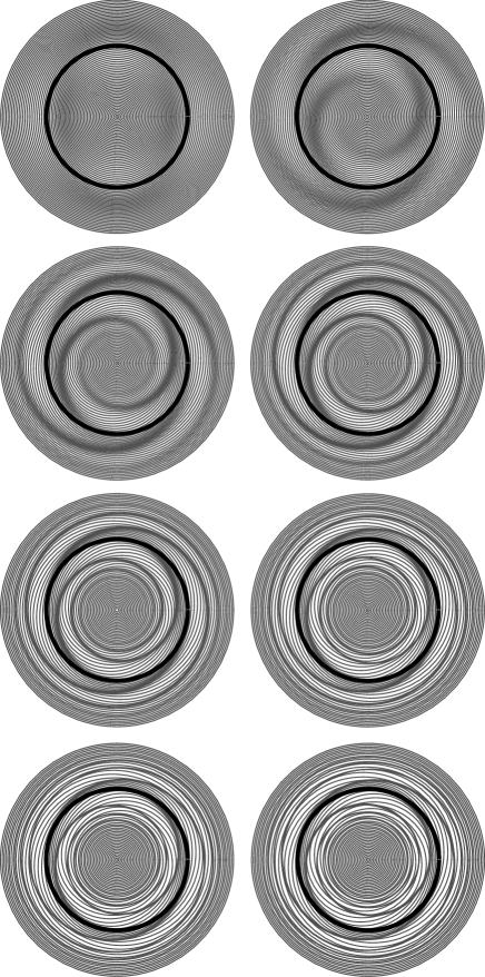
Figure 3: Spiral-arm pattern caused by a perturbation with $m=-2$ around a Kerr black hole with a spin parameter $a=0.5M$. Time advances from left to right and top to bottom. The dark circle shows the circle where $\mu(r)=-2$, i.e. $r_{-2}=4.33M$. The ISCO is $r_{\mathrm{ISCO}}=4.23M$. The spiral pattern is formed by a small-amplitude perturbation in the plane, as described in the text. Since the perturbation is nonzero only in an extremely thin annulus around the black hole, we have cut out the central portions of the disk for clarity. Thus, the center of the polar plot does not correspond to $r=0$, but to $r=r_{-2}-0.015M$, and the plot extends to $r=r_{-2}+0.01M$. The last two snapshots already have formed caustics. Note that although $m=-2$, there are in fact 4 overdense regions because the waves are leading inside $r_{-2}$ and trailing outside $r_{-2}$.

To illustrate the kinematics of the planar density waves, in Figure 3 we plot the $m=-2$ spiral pattern for several times. The initial perturbation was chosen with $\eta(r)=0$ and $\epsilon(r)=10^{-3}M\exp[-(r-r_{-2})^{2}/2\sigma^{2}]$, with $\delta r\sim\sigma=0.003M$. The arm-to-arm displacement period is 0.87 ms. The timestep between the snapshots is 9.3 s, and we have made it to be an exact multiple of the pattern frequency. Therefore, the pattern appears stationary, although it rotates counterclockwise. The winding-up timescale is about 30 s, and the caustic-formation timescale is about 1 minute. We ran similar calculations for a set of perturbations with different $m$, $a$, $\epsilon$ and $\eta$, and we found that our analytical estimates for the winding-up timescale and the lifetime of the pattern are consistent with the numerical results.

Figure 3 verifies the analytic expectations of section 4.2. We see that for $\eta=0$ the spiral pattern for a mode with mode number $m$ has $2|m|$ overdense regions — $|m|$ trailing waves on the outer edge of the perturbation and $|m|$ leading waves on the inner edge in agreement with equation (29). If these overdensities produce comparable modulation of the intensity, then an observer would see a modulation at a frequency $2f_{m}$, exacerbating the problem of matching kinematic density waves to observed black hole QPOs.

If simple density waves cannot explain the observed QPOs, maybe a beat frequency between an orbiting blob and density waves can do the job. Consider a blob of gas orbiting the black hole near $r_{m}$ with angular frequency $\omega_{\phi}(r_{m})$. It must be small and dense enough not to be tidally sheared apart. For $m\leq-1$ the spiral arms will rotate faster than the blob around the disk and thus the blob will be compressed every time the spiral waves pass over it. This leads to a beat frequency in the emission from the blob given by $(\omega_{m}-|m|\omega_{\phi})/2\pi=\omega_{r}/2\pi\equiv f_{r}(r_{m})$, i.e. the radial epicyclic frequency. While the blob remains on one side of $r_{m}$, its beats lead to a flickering frequency of $f_{r}$. If the blob straddles $r_{m}$ hence is overtaken by both leading and trailing density waves, the flickering frequency is $2f_{r}$.

Figure 4: The radial oscillation frequency at $r_{m}$ versus the black hole spin parameter. The uppermost curve corresponds to $m=0$, with $f_{r}$ decreasing as $m$ becomes more negative. The beat frequency between a blob in the disk and a kinematic density wave near $r_{m}$ is either $f_{r}$ or $2f_{r}$ (the frequency being doubled if the blob straddles $r_{m}$). These frequencies appear to be too small to account for observed black hole QPOs.

The radial frequency $f_{r}$ is plotted in Figure 4. The radial frequency in the Kerr metric is less than the azimuthal frequency and goes to zero at the ISCO (corresponding to modes with $m\to-\infty$). This frequency is too low to account for high-frequency QPOs, even if it is doubled.

Figure 5: Low-$m$ sets of frequencies having approximately a $3:2$ ratio. The curves are labeled by the appropriate ratios of $f_{m,|m|}$ for density waves or $f_{r,|m|}$ for blob-wave beat frequencies (in all cases $|m|\leq 0$). Ratios of $f_{m}/f_{r}$ exceed 2.0 except for the special case $f_{m,0}=f_{r,0}$. Although the pairs of modes with $m=-2$ and $m=-3$ have ratios close to 1.5 over a wide range of spin parameter, the actual frequencies are discrepant with observations.

Maybe the black hole mass estimates are in error. If so, the predicted frequencies are wrong but frequency ratios are robust. Thus in Figure 5 we plot all frequency ratios of low-$m$ modes that are close to 1.5. Both the density wave modulation frequencies $f_{m}$ and the radial (blob-wave beat) frequencies $f_{r}$ are included. The only ratios that come close to 1.5 are the pairs with $m=-3$ and $m=-2$. However, the density wave frequencies are too high (the lower frequency is at least 2500 Hz for one solar mass) and the beat frequencies are too low (the lower frequency is less than 420 Hz or 840 Hz if it is doubled) compared with the observed range 1100 to 2000 Hz. The nearest frequency match occurs for spiral density waves with $m=-2$ for $a/M=0$, which would require that the black hole masses be about 25% larger than the upper range of observational estimates. For GRS 1915+105, for example, the lower 113 Hz QPO could be explained by $f_{m,-2}$ if the black hole mass were 22 $M_{\odot}$. The frequency ratio $168/113$ is close to $f_{m,-3}/f_{m,-2}=1.47$. However, the spiral density wave model also predicts modulation at frequencies twice as high (from the combination of inner leading and outer trailing arms), which has not been seen.

Figure 6: The winding up timescale for spiral density waves (the uppermost curve corresponds to $m=0$), giving an order of magnitude estimate of their lifetime in minutes. The lifetimes are much longer than they need to be to produce the observed widths of the QPO spectral peaks.

For completeness we present in Figure 6 the lifetimes of various modes to winding up. The lifetimes must be at least 10 times the inverse frequency in order that mode decay not broaden the peaks in the power spectrum to a lower $Q$ value than is observed. However, this condition is very easily satisfied for modes concentrated near the discrete radii $r_{m}$. The broadening of the timing peaks is probably not due to finite mode lifetime unless the modes extend in radius a significant fraction of the distance to the next discrete mode radius $r_{m}$.

In addition to the beating of a blob with a wave, one might consider the nonlinear interaction between waves of different pattern speeds. However, this leads nowhere because the pattern (or modulation) speed is a function of radius, and spiral density waves of different mode number have different frequencies only because they are localized at different radii.

The application to Kerr has until now considered only planar perturbations. Vertical perturbations can also be excited and are long-lived when concentrated at the discrete radii $r_{n}$ such that $\nu(r_{n})=n$. For the Kerr metric there are only two solutions outside the ISCO:

1. For $a/M>0.9524$ there exists a solution with $n=0$ at $r_{0}\approx 1.9M$. The frequencies are $f_{\theta}=\Omega_{m}/2\pi=4.9$ kHz, with a winding-up timescale of about $\tau=2$ min for $\delta r\sim 0.01M$.

2. For $a/M>0.9987$ there exists a second solution with $n=-1$ at $r_{-1}\approx 1.2M$. The frequencies are $f_{\theta}=2.7$ kHz, $\Omega_{m}/2\pi=16.5$ kHz, with a winding-up timescale of about $\tau=0.4$ min for $\delta r\sim 0.01M$.

Because these modes occur outside the ISCO only for $a/M$ close to maximal, the mode radii and frequencies are nearly constant over the small range of black hole spin where they exist. Given the very narrow range of spins for which these long-lived warps exist, and given their very high frequencies, they are likely to be observationally unimportant.

At larger radii and for smaller black hole spins, the lifetime of vertical waves becomes relatively large even though $\mu$ and $\nu$ are not integers. To order of magnitude the winding time multiplied by mode frequency is $\sim\mu\omega_{m}\tau_{w}\sim(r/\delta r)$ and similarly for the vertical modes. Also, the horizontal and modulation frequencies become comparable: for the same mode number, $0.9\lesssim\omega_{m}/\Omega_{m}<1$ for radii corresponding to pattern frequencies in the range $10^{-4}$ Hz to $10^{3}$ Hz (multiplied by $M_{\odot}/M$). This frequency range includes the low-frequency QPOs seen in the soft power-law state of black hole binaries (Remillard & McClintock, 2006). The QPO frequency varies with X-ray flux, implying that the modulation does not arise at a fixed radius (unlike the high-frequency QPOs).

One explanation for the low-fequency QPOs is Lense-Thirring precession (Stella et al. 1999, Schnittman et al. 2006), with modulation speed $\Omega_{LT}=\omega_{\phi}-\omega_{\theta}$. At large radii, $\nu(r)\to 1$, so vertical density waves with $n=1$ are long-lived and have pattern speed equal to $\Omega_{LT}$. However, planar perturbations have $\mu(r)\to 1$ and are comparably long-lived. Therefore, either planar (spiral waves) or vertical waves (warps) are candidate explanations for low-frequency QPOs, and they have practically the same frequencies and lifetimes. Instead of having no density wave solution consistent with observations (the situation for high-frequency QPOs), the low-frequency QPOs have a plethora of kinematic solutions with little to distinguish them.

7 Conclusions

Starting with a simple kinematical consideration — fluid streamlines should not intersect — we were able to classify all long-lived linear perturbations in pressureless thin accretion disks in generic potentials including the Kerr metric. The result is a set of patterns (planar spiral arms, vertical warps, and linear combinations) whose mode functions are concentrated at discrete radii satisfying a simple condition: the pattern frequency for non–self-intersecting orbits must be approximately constant over a range of radii, i.e. its derivative with respect to radius must vanish. This condition automatically picks out discrete set of frequencies for modes with a long lifetime against winding up. The lifetimes are $O(r/\delta r)^{2}$ oscillation periods where $\delta r$ is the radial extent of the mode.

Although our treatment neglected pressure, the results are in excellent agreement with the diskoseismic $g$-modes investigated by Perez et al. (1997), when the sound speed is much less than the orbital speed. Our treatment, based on the epicyclic approximation, is much simpler than the solution of the relativistic fluid equations.

One of our goals was to investigate the possibility of explaining the $3:2$ ratio in high-frequency quasi-periodic oscillations observed in accreting black hole binaries. Our model gives several mode pairs with a frequency ratio close to 1.5 for a wide range of black hole spin. This result is a direct consequence of the discrete radii at which the spiral patterns exist. However, we cannot recover naturally the correct frequencies unless the black hole mass estimates are seriously in error. Planar spiral density waves have frequencies too high, while the beat frequency between a blob and these waves is too low, compared with the observed frequencies. Moreover, the best matches follow for modes with $|m|=2$ and $|m|=3$, with no explanation for the failure to observe the mode with $|m|=1$.

Because our analysis classified all long-lived perturbations of pressureless disks, the failure to reproduce the observed high-frequency quasi-periodic oscillations implies that pressure or other non-gravitational forces (e.g. magnetic stresses or radiation pressure) must be important in producing the QPOs.

Based on the diskoseismic results, we would expect that small non-gravitational forces do not significantly change the mode frequencies. Large non-gravitational forces would thicken the disk and might destroy the coherence and longevity of modes, although this remains to be seen. Even so, some mechanism is needed to pick out discrete frequencies of the high-frequency QPOs.

These results make more attractive the possibility that nonlinear coupling between modes, e.g. parametric resonance, is responsible for selecting the frequency ratios (Abramowicz & Kluźniak 2001; Rebusco 2004). One approach to investigating this process is to carry the perturbation methods of the current paper to one higher order, to include a coupling between radial and vertical oscillations.

References

- Abramowicz & Kluźniak (2001) Abramowicz, M. A., & Kluźniak, W. 2001, A&A, 374, L19
- Amin & Frolov (2006) Amin, M. A., & Frolov, A. V. 2006, MNRAS, 370, L42
- Binney & Tremaine (1987) Binney, J., & Tremaine, S. 1987, Galactic Dynamics (Princeton University Press)
- Homan et al. (2005) Homan, J., Miller, J. M., Wijnands, R., van der Klis, M., Belloni, T., Steeghs, D., & Lewin, W. H. G. 2005, ApJ, 623, 383
- Kalnajs (1973) Kalnajs, A. J. 1973, Proc. Ast. Soc. Aus., 2, 174
- Lee et al. (2004) Lee, W. H., Abramowicz, M. A., & Kluźniak, W. 2004, ApJ, 603, L93
- Lindblad (1957) Lindblad, B. 1957, Stockholm Obs. Ann., 9
- Miller et al. (2001) Miller, J. M., Wijnands, R., Homan, J., Belloni, T., Pooley, D., Corbel, S., Kouveliotou, C., van der Klis, M., & Lewin, W. H. G. 2001, ApJ, 563, 928
- Perez et al. (1997) Perez, C. A., Silbergleit, A. S., Wagoner, R. V., & Lehr, D. E. 1997, ApJ, 476, 589
- Rebusco (2004) Rebusco, P. 2004, PASJ, 56, 553
- Remillard (2004) Remillard, R. A. 2004, in AIP Conf. Proc. 714, X-Ray Timing 2003: Rossi and Beyond, ed. P. Kaaret, F. K. Lamb, & J. H. Swank (Melville, NY: AIP), 13
- Remillard & McClintock (2006) Remillard, R. A., & McClintock, J. E. 2006, ARA&A, 44, 49
- Rezzolla et al. (2003) Rezzolla, L., Yoshida, S., Maccarone, T. J., & Zanotti, O. 2003, MNRAS, 344, L37
- Schnittman (2005) Schnittman, J. D. 2005, ApJ, 621, 940
- Schnittman & Bertschinger (2004) Schnittman, J. D., & Bertschinger, E. 2004, ApJ, 606, 1098
- Schnittman et al. (2006) Schnittman, J. D., Homan, J., & Miller, J. M. 2006, ApJ, 642, 420
- Stella et al. (1999) Stella, L., Vietri, M., & Morskink, S. M. 1999, ApJ, 524, L63
- Strohmayer (2001) Strohmayer, T. E. 2001, ApJ, 552, L49
- Toomre (1977) Toomre, A. 1977, ARA&A, 15, 437
- Wagoner et al. (2001) Wagoner, R. V., Silbergleit, A. S., & Ortega-Rodríguez, M. 2001, ApJ, 559, L25