Structure of metastable 2D liquid helium

Abstract

We present diffusion Monte Carlo (DMC) results on a novel metastable, superfluid phase in two-dimensional ⁴He at densities higher than 0.065Å^-2. The state is above the crystal ground state in energy and it has anisotropic, hexatic orbital order. This implies that the liquid–solid phase transition has two stages: A second order phase transition from the isotropic superfluid to the hexatic superfluid, followed by a first order transition that localizes atoms into the triangular crystal order. This metastable hexatic phase offers a natural explanation for the superflow in the supersolid ⁴He and the possibility of a Kosterlitz-Thouless type phase transition with increasing temperature.

Metastable states are transient, excited states that have a relatively long lifetime, and may appear in the absence of an external disturbance that would trigger the transition to the ground state. Three–dimensional helium has a metastable high–density (pressure) liquid phase, observed in laboratory experiments by Ishiguro et al.Ishiguro et al. (2006) and Werner et al.Werner et al. (2004). The liquid phase is measured up to 160 bar - far above the liquid solid freezing pressure of 25.3 bar. Also Pearce et al. Pearce et al. (2004) observed metastable liquid at pressures up to 40 bar in helium immersed in gelsil pores. These types of metastable states are typical for a first order phase transition where latent heat must be released to make the transition from liquid to solid phase. Diffusion Monte Carlo (DMC) simulations by Vranjes et al.Vranješ et al. (2005) confirmed that a metastable state is superfluid with a finite condensate fraction and has a roton minimum in the excitation spectrum up to 275 bar, but no upper limit to this behavior is proposed.

Variational calculations of both 2D and 3D helium liquid suggest that the isotropic low–density liquid state becomes unstable against formation of an anisotropic liquid state before the solidification pressure is reached Halinen et al. (2000); Apaja et al. (2000). This phase transition is of second order. No latent heat is required in the transition and thus it can not support metastable states. In classical fluids the corresponding anisotropic phase is named hexatic phase after the proposal made by Halperin and NelsonHalperin and Nelson (1979). Up to now, very large scale simulations Jaster (1999); Mak (2006) have been performed with a simple two-dimensional hard disk fluid to verify the theory of the continuous phase transition, where hexatic phase is the intermediate phase before the full solid order. These results seem to point toward a weakly first order phase transition.

Observation of the nonclassical rotational inertia (NCRI) by Kim and ChanKim and Chan (2004, 2006) challenged our understanding of the solid ⁴He phase. Since then both experimental and theoretical results seem to conclude that a perfect crystal can not be superfluid Chan (2008); Prokof’ev (2007); Boninsegni et al. (2006); Rittner and Reppy (2006). A strong dependence of the superfluid fraction on crystal annealing supports the idea that some kind of a metastable state could be responsible of these observation. Boninsegni at al.Boninsegni et al. (2006) proposed a glassy phase, but recent experiments on the specific heat at very low temperatures cast some doubts on that proposal Lin et al. (2007). Recently Sasaki et al. Sasaki et al. (2006) have shown that the transport of mass in the supersolid ⁴He can take place along grain boundaries. It requires that boundary layers form a quasi two-dimensional superfluid. The puzzle is that superfluid fraction does not scale with the amount of grain boundaries in the sample. Nevertheless, numerical simulations have shown superflow at grain boundaries Pollet et al. (2007). The superfluid fraction seems to support vortices, which collect ³He impurities Anderson (2007); Kim et al. (2008), and the phase transition to supersolid phase could then be related to the Kosterlitz-Thouless type phase transition. Unusual behavior of the shear modulus in solid ⁴He has also been observed Day and Beamish (2007) at the same temperature range where the supersolidity appears in the torsional oscillator measurements.

In this article we present results on DMC simulation of the two–dimensional ⁴He at zero temperature and show that the hexatic, high-pressure metastable liquid phase exists slightly above the crystal phase in energy. The phase transition from liquid to solid has two stages when the pressure increases. It is triggered by the second order transition from the liquid to the hexatic phase, but then the first order transition to the solid order requires external perturbation.

The ground state properties of zero temperature 2D ⁴He have been studied using Monte Carlo methods by Giorgini et al.Giorgini et al. (1996) and by Whitlock et al.Whitlock et al. (1988), who find that the ground state at high densities is a triangular solid phase. Helium layers on a substrate, such as graphite, and in porous media have been thoroughly studied using theory Clements et al. (1993); Whitlock et al. (1998); Apaja and Krotscheck (2003) and experiments Lauter et al. (1992). The full phase diagram at finite temperature has been calculated using path integral Monte Carlo by Gordillo and Ceperley Gordillo and Ceperley (1998). Also the change in the angular order in the liquid–solid transition has been discussed using the variational shadow wave function Krishnamachari and Chester (2000). Our new result complements those properties with a metastable superfluid state, which has the hexatic two-particle structure.

We first describe how structural properties were obtained from the simulation. Diffusion Monte Carlo Reynolds et al. (1982) is a zero–temperature method that uses a large number (in this work $\sim 500-1000$) of independent $N$–atom simulations, walkers, to statistically represent an imaginary time (marked $\tau$) evolution process to a wave function $\Psi(\tau)$. In principle this projects out the excited states and one proceeds to sample the properties of the ground state $\phi_{0}$. In a simulation metastability arises if it is improbable that one sees the asymptotic result $\Psi(\tau)\to\phi_{0}$ within the limited simulation time. In other words, there may only be a very narrow random–walk path that takes the evolution to the ground state. Statistics is always improved with importance sampling and a chosen trial state. With importance sampling one biases the random walk, usually to the effect that the ground state is reached faster. For example, if one imposes a triangular solid symmetry to the trial state one obtains the properties of the premeditated solid phase.Whitlock et al. (1988)

For helium we use the McMillan trial wave function, modulated with an angular component,

$$\varphi_{T}=\prod_{i<j}\exp\left[\alpha\frac{\cos(m\phi_{ij})-1}{r_{ij}}\right]\exp\left[-\left(\frac{r_{ij}}{\beta}\right)^{\mu}\right]\;.$$ (1)

The variational constants are $\beta\sim 3.3$ Å and $\mu=4$. Here $m$ is an even integer and the angle between atoms at ${\bf r}_{i}$ and ${\bf r}_{j}$ is defined $\cos(\phi_{ij})=\frac{{\bf r}_{j}-{\bf r}_{i}}{r_{ij}}\cdot\hat{\bf e}_{0}$, with respect to a reference direction $\hat{\bf e}_{0}$ and $r_{ij}=|{\bf r}_{i}-{\bf r}_{j}|$ is the distance between the atoms $i$ and $j$. The amplitude of the trial angular structure is $\alpha\sim 0-0.6$.2D- (a) This wave function has no crystalline order and atoms are not fixed to lattice sites, contrary to the Nosanow type solid trial state. Also the anisotropic trial state is not the same as using, say, a substrate potential, because the liquid structure cannot ignore the latter and a potential induces a global order, and not just a local one, around each atom. Here we are not forcing anything upon the 2D liquid itself, merely adding a possibility to measure the degree of anisotropy from the simulation. Within statistical error, the energy and the radial distribution function of the metastable state are independent of the trial state.

The reference direction $\hat{\bf e}_{0}$ is set externally, which enables us to see if the high–density liquid orients itself to the direction set by the trial wave function. In short, we estimate how strongly the liquid binds to the globally defined orientation. From the simulation we determine the pair distribution, expanded as

$$g({\bf r})=\sum_{m=0}^{\infty}g_{m}(r)\exp{(im\theta)}\;,$$ (2)

where $m$ is even and $\cos(\theta)=\hat{\bf r}\cdot\hat{\bf e}_{0}$. In this work we keep terms up to $m=12$. We measure the pair distribution rather than the momentum space static structure function, because we expect to see only a very small effect and $g_{m}(r)$ can be accurately deduced from the simulation.

If the trial state is still a liquid, why should the angular part make any difference? The angular part serves a dual purpose, in close relation to the way quantities are measured in DMC. First, a well–known fact is that if the trial state is not too far from the eigenstate $\phi$, one can approximate the expectation values of operator ${\cal A}$ by the so–called extrapolated estimator, $\langle\phi|{\cal A}|\phi\rangle\approx 2\langle\phi|{\cal A}|\varphi_{T}\rangle-\langle\varphi_{T}|{\cal A}|\varphi_{T}\rangle$, where $\langle\phi|{\cal A}|\phi\rangle$ is what we want to know, $\langle\phi|{\cal A}|\varphi_{T}\rangle$ is what the average over walkers gives, and $\langle\varphi_{T}|{\cal A}|\varphi_{T}\rangle$ is the value in the trial state. This implies that even if there is no angular order in $\phi$, the walkers simulate roughly half of the order we put in the trial state $\varphi_{T}$. As a result the trial state gently biases the walkers to favor a given globally oriented local anisotropy. In this respect the trial state acts as a perturbation. The extrapolation or the forward walking algorithm discussed below removes this perturbation from the final expectation values.

The second reason for using the angular part is that it enables us to measure how this “perturbation” affects the high–density liquid in coordinate space. To see why, let us first assume that the metastable liquid indeed has a global angular order with respect to some fixed external (laboratory) direction, but we use a spherically symmetric trial state. Then in the DMC simulation each walker picks up a different, randomly chosen orientation, which, over a large number of walkers, averages to zero. This is the reason why we need a non–zero angular order in the trial state in order to see one in $\phi$ when using a coordinate space observable. The fact that a trial state, or importance sampling in general, can be used to actually make a quantity observable in a Monte Carlo simulation is not frequently mentioned in standard texts.

If available, we always use unbiased estimators, since extrapolated estimators are known to give systematic error, especially for structural quantities like the pair distribution. In this work we apply the algorithm based on forward walking described in Ref. Casulleras and Boronat, 1995. One keeps track on how many asymptotic off-springs a given walker will have, and weights the present situation accordingly. Although the name indicates that these results are unbiased by the trial state, this is not entirely true: as discussed above, without the trial state angular structure there is no chance of observing coordinate space angular order. In our case the unbiased estimators are more like conditional results, valid for a certain fixed amplitude of the angular term in the trial state, and we note in passing that the unbiased and the extrapolated estimators agree well. We have also checked that the period we follow the walkers is long enough so that the asymptotic regime is reached, but not too long to become unstable. Sarsa et al. Sarsa et al. (2000) compared the pair structure of 3D liquid helium obtained using the Path Integral Ground State (PIGS) method and the forward walking DMC algorithm and find that the two methods produce very accurately the same result.

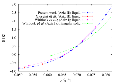
Figure 1: The total energy of 2D helium as a function of density. The present data and the data by Giorgini et al.Giorgini et al. (1996) are computed using DMC with the revised Aziz HFDHE2 potentialAziz et al. (1979) (“Aziz II”). For comparison we show the energies of liquid and triangular solid by Whitlock et al.Whitlock et al. (1988), who used the 1979 version of the Aziz HFDHE2 potential (“Aziz I”).Aziz et al. (1987)

We have done simulations using a quadratic DMC algorithm, using mainly 64 or 120 atoms. Fig. 1 shows the total energy vs. density in the high–density 2D liquid and triangular solid. Notice the two slightly different He-He potentials used in the QMC calculations. Our results agree well with the liquid energies computed by Giorgini et al.,Giorgini et al. (1996) available up to $\rho<0.065$Å^-2. For testing we also reproduced the Aziz-I potential liquid energies reported by Whitlock et al.Whitlock et al. (1988). Trial states with $\alpha$ in the range 0-0.6 gave the same total energies within statistical error bars. Also the spherically symmetric component of the radial distribution function $g(r)\equiv g_{m=0}(r)$ is the same for any trial state angular parameter $\alpha$.

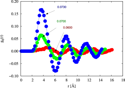
Figure 2: The $g_{m=6}(r)$ component of the pair distribution function at densities $\rho=0.073$, 0.070, and 0.060Å^-2, computed using the same $m=6$ trial state with $\alpha=0.6$ and 64 atoms. The lowest density corresponds to a stable liquid and the two higher ones to the metastable liquid with a hexatic order.

The phase transition from the isotropic to anisotropic liquid generates angular dependence into the pair distribution function $g({\bf r})$. The transition is continuous and the amplitude of the angle dependence increases with increasing density. The angular behavior is determined by the $m=6$ component of the expansion in Eq. (2), which is in agreement with the point group symmetry of the triangular lattice. Fig. 2 shows the component $g_{m=6}(r)$ at three densities near the freezing density, computed using exactly the same trial state. While the stable liquid ($\rho=0.060$Å^-2) is insensitive to the trial state, the metastable liquid shows a clear externally oriented angular structure. The amplitude of the short distance oscillations in $g_{m=6}(r)$ increases with increasing density, but in long distances these oscillations vanish, which means that the system remains in the liquid state. The phase transition is made more apparent in Fig. 3, where we plot the maximum value of $g_{m=6}(r)$ i.e. the amplitude of the first oscillation. We use the same trial wave function at all densities and Fig. 3 shows also the “input amplitude”, computed using variational Monte Carlo (VMC). While the trial wave function gives rise to angular amplitude that slowly increases as the density increases, the DMC data shows a clear onset of angular structure. Above the density $0.065$Å^-2 - remarkably close to the expected freezing density - the $g_{m=6}(r)$ component increases anomalously, yet much less than what would be observed in freezing.2D- (b) The fact that the DMC algorithm reduces the amplitude from above 0.12 in the trial wave function to less than 0.02 at low densities shows how little bias there is, and that the forward walking DMC algorithm is indeed able to remove the trial state angular structure if it is favorable.

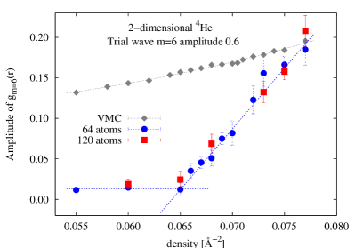
Figure 3: The amplitude of the $g_{m=6}(r)$ component of the pair distribution as a function of density, computed using trial state with the amplitude $\alpha=0.6$. For reference, the points labeled “VMC” show the input trial state $g_{m=6}(r)$ amplitude. The lines are just guides to the eye.

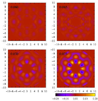
Figure 4: The pair distribution $g({\bf r})$ summing $g_{m}(r)$ from $m=2$ to $m=12$ (without the radial component), as a function of density, computed using a trial state with $\alpha=0.6$. Lighter areas correspond to positive (increased probability) and darker to negative values. The labels in the figures show the densities in units Å^-2. The reference atom is in the middle and the we show a 20 Å by 20 Å box around it.

In the metastable state the pair distribution function $g({\bf r})$ has a sixfold symmetry, depicted in Fig. 4. To make the modulation more visible we have subtracted the uninteresting radial part $g(r)$. One might erroneously conclude that the apparent sixfold symmetry seen in the pair distribution around every atom adds up to having a triangular solid. However, a mere modulation in the probability (relative to random) does not warrant that conclusion. The full spatial crystal order requires releasing of latent heat leading to the triangular structure in the single particle densityGernoth (2000). Here the single particle density stays constant.

In the high—density, metastable ⁴He the angular component $g_{m=6}(r)$ of the pair distribution function grows above the freezing density, unlike any other component. To exclude the possibility that this is an artifact due to the $m=6$ symmetry put into the trial state, we repeated the calculation using a four–fold symmetry in $\varphi_{T}$; in that case no anomalous increase in $g_{m=4}(r)$ was observed. In our DMC calculations we used a periodically repeated square box, which is not commensurate with a triangular lattice and also won’t enhance the sixfold symmetry component. According to our results the metastable state is superfluid, although the DMC method is not ideal for measuring the long range order in the one-particle density matrix. We find no abrupt change in that long range order when the density crosses the freezing density. The decay of the long range tail remains very slow with increasing density as one would expect from a 2D liquid ⁴He.

In conclusion we have shown that a novel metastable state in two-dimensional ⁴He exists at high densities. It has the hexatic orbital symmetry, but homogeneous single particle density. The superfluidity of that state may explain the nonclassical rotational inertia observed in supersolids. As the state is metastable the crystal growth process determines sensitively the fraction of ⁴He, which remains in the superfluid phase. In rapid freezing of ⁴He within a narrow annular region by Rittner and Reppy created a large superfluid fraction of a metastable state up to 20 % in the sample Rittner and Reppy (2007). Annealing removed the metastable state and the nonclassical rotational inertia state almost completely disappeared Rittner and Reppy (2006). We like to draw attention to a similar metastable state in three dimensional ⁴He where the ultrasound shock wave experiments pressurized ⁴He far beyond the freezing density, and yet ⁴He remained superfluid.

We thank E. Krotscheck for many discussions and his hospitality during our stay in the Johannes Kepler University in Linz, were part of the computations were performed using the local computer resources. We are also grateful to J. Boronat for stimulating discussions.

References

- Ishiguro et al. (2006) R. Ishiguro, F. Caupin, and S. Balibar, Europ. Lett 75, 91 (2006).
- Werner et al. (2004) F. Werner, G. Beaume, A. Hobeika, S. Nascimbene, C. Herrman, F. Caupin, and S. Balibar, J. Low Temp. Phys. 136, 93 (2004).
- Pearce et al. (2004) J. V. Pearce, J. Bossy, H. Schober, H. R. Glyde, D. R. Daughton, , and N. Mulders, Phys. Rev. Lett. 93, 145303 (2004).
- Vranješ et al. (2005) L. Vranješ, J. Boronat, J. Casulleras, and C. Cazorla, Phys. Rev. Lett. 95, 145302 (2005).
- Halinen et al. (2000) J. Halinen, V. Apaja, K. A. Gernoth, and M. Saarela, J. Low Temp. Phys. 121, 531 (2000).
- Apaja et al. (2000) V. Apaja, J. Halinen, and M. Saarela, Physica B 284-288, 29 (2000).
- Halperin and Nelson (1979) B. I. Halperin and D. R. Nelson, Phys. Rev. B 19, 2457 (1979).
- Jaster (1999) A. Jaster, Phys. Rev. E 59, 2594 (1999).
- Mak (2006) C. H. Mak, Phys. Rev. E 73, 065104 (2006).
- Kim and Chan (2004) E. Kim and M. H. W. Chan, Nature 427, 225 (2004).
- Kim and Chan (2006) E. Kim and M. H. W. Chan, Phys. Rev. Lett. 97, 115302 (2006).
- Chan (2008) M. H. W. Chan, Science 319, 1207 (2008).
- Prokof’ev (2007) N. V. Prokof’ev, Adv. Phys. 56, 381 (2007).
- Boninsegni et al. (2006) M. Boninsegni, N. Prokof’ev, and B. Svistunov, Phys. Rev. Lett. 96, 105301 (2006).
- Rittner and Reppy (2006) A. S. C. Rittner and J. D. Reppy, Phys. Rev. Lett. 97, 165301 (2006).
- Lin et al. (2007) X. Lin, A. C. Clark, and M. H. W. Chan, Nature 449, 1025 (2007).
- Sasaki et al. (2006) S. Sasaki, R. Ishiguro, F. Caupin, H. J. Maris, and S. Balibar, Science 313, 1098 (2006).
- Pollet et al. (2007) L. Pollet, M. Boninsegni, A. B. Kuklov, N. V. Prokof’ev, B. V. Svistunov, and M. Troyer, Phys. Rev. Lett. 98, 135301 (2007).
- Anderson (2007) P. W. Anderson, Nature Physics 3, 160 (2007).
- Kim et al. (2008) E. Kim, J. S. Xia, J. T. West, X. Lin, A. C. Clark, and M. H. W. Chan, Phys. Rev. Lett. 100, 065301 (2008).
- Day and Beamish (2007) J. Day and J. Beamish, Nature 450, 853 (2007).
- Giorgini et al. (1996) S. Giorgini, J. Boronat, and J. Casulleras, Phys. Rev. B 54, 6099 (1996).
- Whitlock et al. (1988) P. A. Whitlock, G. V. Chester, and M. H. Kalos, Phys. Rev. B 38, 2418 (1988).
- Clements et al. (1993) B. E. Clements, J. L. Epstein, E. Krotscheck, and M. Saarela, Phys. Rev. B 48, 7450 (1993).
- Whitlock et al. (1998) P. A. Whitlock, G. V. Chester, and B. Krishnamachari, Phys. Rev. B 58, 8704 (1998).
- Apaja and Krotscheck (2003) V. Apaja and E. Krotscheck, Phys. Rev. Lett. 91, 225302 (2003).
- Lauter et al. (1992) H. J. Lauter, H. Godfrin, V. L. P. Frank, and P. Leiderer, Phys. Rev. Lett. 68, 2484 (1992).
- Gordillo and Ceperley (1998) M. C. Gordillo and D. M. Ceperley, Phys. Rev. B 58, 6447 (1998).
- Krishnamachari and Chester (2000) B. Krishnamachari and G. V. Chester, Phys. Rev. B 61, 9677 (2000).
- Reynolds et al. (1982) P. J. Reynolds, D. M. Ceperley, B. J. Alder, and W. A. Lester, J. Chem. Phys. 77, 5593 (1982).
- 2D- (a) As Fig. 3 shows, states with larger angular order are variationally far from the final state, and one needs excessively many walkers to remove the statistical bias.
- Casulleras and Boronat (1995) J. Casulleras and J. Boronat, Phys. Rev. B 52, 3654 (1995).
- Sarsa et al. (2000) A. Sarsa, K. E. Schmidt, and W. R. Magro, J. Chem. Phys. 113, 1366 (2000).
- Aziz et al. (1979) R. A. Aziz, F. R. W. McCourt, and C. C. K. Wong, J. Chem. Phys. 70, 4330 (1979).
- Aziz et al. (1987) R. A. Aziz, V. P. S. Nain, J. C. Carley, W. J. Taylor, and G. T. McConville, Mol. Phys. 61, 1487 (1987).
- 2D- (b) We also saw few cases of freezing with rapid increase in the angular order, similar to one reported in Ref. Krishnamachari and Chester, 2000.
- Gernoth (2000) K. A. Gernoth, Ann. Phys. 61, 285 (2000).
- Rittner and Reppy (2007) A. S. C. Rittner and J. D. Reppy, Phys. Rev. Lett. 98, 175302 (2007).