Cascading to the MSSM

Abstract

The MSSM can arise as an orientifold of a pyramid-like quiver in the context of intersecting D-branes. Here we consider quiver realizations of the MSSM which can emerge at the bottom of a duality cascade. We classify all possible minimal ways this can be done by allowing only one extra node. It turns out that this requires extending the geometry of the pyramid to an octahedron. The MSSM at the bottom of the cascade arises in one of two possible ways, with the extra node disappearing either via Higgsing or confinement. Remarkably, the quiver of the Higgsing scenario turns out to be nothing but the quiver version of the left-right symmetric extension of the MSSM. In the minimal confining scenario the duality cascade can proceed if and only if there is exactly one up/down Higgs pair. Moreover, the symmetries of the octahedron naturally admit an automorphism of the quiver which solves a version of the $\mu$ problem precisely when there are an odd number of generations.

1 Introduction

At present, no experiment has verified any signature unique to string theory.  Given that the LHC will soon directly probe physics beyond the Standard Model, it is natural to ask whether string theory can produce any concrete prediction. On first inspection, even one specific low energy prediction would appear unlikely because string theory is a theory of quantum gravity and as such its most novel predictions will involve energy scales close to the string or the fundamental Planck scale.  In order to avoid conflict with observation, this scale is typically taken to be far above the TeV scale.

In the context of grand unified field theories, however, the advent of Heterotic string theory [1] and the 4d gauge theory structure resulting from its Calabi-Yau compactifications [2] suggested rather limited ways that the matter content of the Standard Model could emerge from a consistent theory of quantum gravity.  This raised theoretical hopes that perhaps string theory would predict a relatively robust structure for gauge theory and matter structure from simple topological and representation theoretic criteria.

But this hope has been dashed with the advent of the duality era in string theory which demonstrates rather convincingly the existence of a large class of non-perturbative string compactifications with a diverse range of gauge groups and matter content. Thus an exponentially large number of solutions can be constructed –the string landscape– which look more or less like the Standard Model (for a review see [3]). Of course this is not to say that any consistent quantum field theory will embed in a consistent fashion inside a quantum theory of gravity.  It is therefore important to delineate the boundary between field theories which possess such an embedding and those which simply fall in a more general swampland of effective field theories (see e.g. [4]). These constraints typically arise because not every local geometry leading to a 4d QFT can appear as part of a compact internal geometry.  Nevertheless, such constraints appear to be difficult to narrow down with our present understanding of string theory.  It is thus natural to ask whether local aspects of string theory impose any further constraints on observed QFT’s and further, whether symmetries natural from the perspective of string theory possess a low energy remnant in the effective field theory.  More broadly, we ask: Are there any field theories which are more distinguished among others, from a stringy viewpoint?

There seems to be one regard in which considerations following from local geometry produce a robust prediction.  Indeed, it does not appear possible to engineer arbitrary matter content from a configuration of D-branes.  For example, for $U(N)$ gauge groups, no representation of rank higher than two appears for generic $N$.  Another example is in the context of $U(N)\times U(k)$ type groups:  In oriented string theories the matter fields which are charged under both groups always appear to transform as bifundamentals $(N,\overline{k})$ or $(\overline{N},k)$.  This is the case, for example, in the context of intersecting D-branes and the matter localized at their intersection [5].

Quite remarkably, the matter content of the Standard Model compactly fits in such rank two representations.  It is therefore natural to expect a local string realization of this type of theory.  Representative papers on realizing the Standard Model from a D-brane probe of a Calabi-Yau singularity may be found in [6, 7, 8].  There is also a large body of work on intersecting D-brane models.  For recent reviews and a more complete list of references in the context of intersecting brane configurations, see [9, 10, 11].  Modulo issues pertaining to tadpole cancellation from orientifold planes, any such D-brane realization should also possess a smooth large $N$ limit.

In some cases, this large $N$ limit connects directly to a low energy gauge theory with much smaller rank.  Indeed, this connection is known in a number of cases in string theory and involves the concept of a duality cascade. The aim of this paper is to investigate this question in the context of minimal realizations of the Standard Model in terms of quiver theories. We note, however, that this approach has one disadvantage because it presupposes that the unification of the gauge coupling constants in the supersymmetric context is an accident. As we shall explain later, GUTs do not appear to naturally arise from D-brane constructions.

We now explain why the concept of a duality cascade is particularly appealing in the context of D-brane realizations of the Standard Model.  An ubiquitous theme in string (motivated) phenomenology is the translation of field theoretic data into geometry.  Prominent examples are the engineering of Standard Model-like gauge theories via singular geometries and D-branes, and the dual representation of the gauge hierarchy in terms of warped extra dimensions. The holographic interplay between gauge and gravitational degrees of freedom underscores the crucial rôle D-branes play in establishing a string-theoretic link between gauge theory and gravity.  Indeed, a large number of D-branes will melt into geometry. This process can in fact be done continuously [12].  Starting from a configuration with a large number of D-branes which is captured by the geometry, at distances closer to the tip of the cone, the dual description in terms of a stack of branes will cause the initially large number of branes to sequentially decrease until only a finite number of branes are left at the ‘bottom’ of the geometry. In the dual gauge theory this corresponds to a duality cascade whereby a series of Seiberg dualities sequentially decreases the ranks of the gauge group as the RG flow proceeds from the UV to IR so that deep in the IR the resulting gauge groups have small finite rank.

Indeed, this is very natural for phenomenology: In the IR, which is the scale at which the Standard Model has been directly probed, we observe $SU(3)\times SU(2)\times U(1)$ gauge symmetry. Could it be that at higher energy scales, the ranks of the gauge groups increase, leading ultimately near the Planck scale simply to gravity?

We will see that this scenario can be realized. In fact, quite surprisingly we find that there is very little choice in the minimal realization of a cascading structure leading to the Standard Model at the bottom of the cascade.  The minimal quiver realization of the Standard Model involves an orientifold of a “covering” quiver theory which has the shape of a pyramid with the lift to the cover of the weak group $SU(2)_{L}$ at the apex of the pyramid.  Just as in the Klebanov Strassler cascade, we expect additional nodes to disappear near the end of the cascade.  Indeed, it turns out that in order to get a cascading structure, one must minimally add one extra node which enhances the already symmetric pyramid to an octahedron.  In this case, orientifolding the covering theory by a 180 degree rotation along its symmetry axis leads to an essentially unique cascading model for the Standard Model.  Depending on how the cascade terminates, there are two further possible refinements.

The most direct analogue of the Klebanov Strassler cascade corresponds to the case where the rank of the gauge group factor on the extra node depletes to zero at the bottom of the cascade.  In this case it turns out quite surprisingly that we need exactly one up/down Higgs pair for the cascade to proceed!  Rather than requiring that the extra node confine at the bottom of the cascade, it is also possible to Higgs the quiver theory before the ranks of any node completely depletes so that two of the quiver nodes collapse to a single quiver site. Prior to Higgsing, the corresponding quiver theory is in fact nothing but the quiver of the left-right symmetric extension of the MSSM.

We note that the original idea that the Standard Model may lie at the bottom of a cascade is not new and has been advocated, for example, in [12, 13].  Although the explicit models we shall consider do not have a conformal limit, more generally, a cascade will proceed by perturbing the ranks of a given conformal field theory.  Indeed, the idea of approaching a conformal limit in the ultraviolet in the context of quiver realizations of the Standard Model has been studied as a potential solution to the hierarchy problem in [14]. Furthermore, string theory constructions with semi-realistic Standard Model vacua at the bottom of a cascade with a holographic dual have been realized in [15].

The rest of this paper is organized as follows.  In section 2 we review the relation between D-branes and the associated $U$-type quivers, as well as their orientifolds and the resulting $U/USp/SO$-type quivers. In this same section we summarize how the Standard Model embeds in a minimal quiver consistent with D-brane constructions in string theory. We call this minimal quiver realization of the Standard Model the MQSM.  We next review in section 3 how to Seiberg dualize quiver gauge theories and how sequences of Seiberg dualities give rise to cascading gauge theories.  Beginning in section 4 we commence our analysis of ways in which the MQSM can sit at the bottom of a periodic duality cascade. We identify two minimal scenarios by which a cascading quiver theory with four quiver nodes can Higgs or confine down to the three node MQSM.  In section 5 we present a left-right symmetric cascading gauge theory that reaches the MQSM via Higgsing.  In section 6 we present a partial classification of cascading four node quivers that terminate at the MQSM when the extra node confines.  Some technical parts of this section are deferred to Appendices A and B.  The combinatorics of possible cascades in this latter approach is more intricate and places strong constraints on candidate cascades.  In fact, we find that the requirement of a repeating cascade structure requires the presence of exactly one light up/down Higgs pair!  Quite unexpectedly, we find that at intermediate stages of the cascade, the structure of the quiver theories in the Higgsing and confining scenarios is nearly identical.  Indeed, in section 7 we explain how the two cascades can be mapped to each other by adding or integrating out vector-like pairs.  This is reassuring in that it suggests a robust extension of the MQSM which admits a periodic cascade structure.  With the intermediate stages of the cascade analyzed, we next describe in greater detail the behavior of the two cascading scenarios near the bottom of the cascade in section 8.  Proceeding from the IR to the UV, we find that whereas the scales of dualization for the Higgsing scenario quite flexibly accommodate a range of possibilities, in the minimal version of the confining scenario much of the cascade would be forced to dualize above the Planck scale.  We present a minimal modification designed to accelerate the running of couplings and comment on ways in which supersymmetry breaking can arise in the low energy theory.  Combining the above analysis, in section 9 we discuss in more detail the structure of the running of the coupling constants and the fact that in either approach we hit a duality wall at finite scale.  In section 10 we discuss the possibility of realizing the above cascade using a D-brane construction.  Section 11 discusses in what sense the cascade distinguishes the matter content and gauge groups of the MSSM from other possible cascade endpoints. Finally, in section 12 we conclude and discuss directions for future research.

2 D-branes, Quivers and the MQSM

In order to make the discussion to follow more self-contained, and hopefully of interest to a broader range of readers, in this section we review the types of gauge theories which can in principle arise from supersymmetric D-brane constructions.  For more detailed reviews we refer to [9, 10, 11]. Although the restrictions on the matter content and gauge group types we discuss will continue to hold in the context of non-supersymmetric gauge theories, in order to apply the above considerations to cascading gauge theories we shall always restrict our analysis to theories which preserve at least $\mathcal{N}=1$ supersymmetry.

2.1 Oriented Theories

We first recall how gauge symmetry arises in the context of D-brane constructions.  In a sigma-model description, a D-brane is a defect in spacetime where an open string can end.  In the presence of $N$ D-branes, each endpoint of an oriented open string is labelled by an additional Chan-Paton index $i=1,...,N$ indicating which brane a string can end on.  When all of the branes form a single stack, the resulting open string modes transform in the adjoint representation of a $U(N)$ gauge group.  Quantizing such an open string yields a vector multiplet and possibly additional adjoint chiral fields at the massless level.  In all cases, we consider D-branes which fill our four dimensional spacetime and wrap some internal cycle of a compactified six dimensional manifold in the extra dimensions.  Assuming that the internal cycle has volume $V$, the gauge coupling of the four dimensional effective theory is:

$$\frac{1}{g_{YM}^{2}}\sim\frac{V}{g_{s}}\text{.}$$ (1)

Chiral matter in general arises from topologically stable intersections between two stacks of branes in the internal dimensions. Both stacks of branes fill space-time, and intersect at a finite number of points in the internal six-manifold. As an example, in type IIA string theory, consider a stack of $N_{1}$ D6-branes and another stack of $N_{2}$ D6-branes which both fill the spacetime $\mathbb{R}^{3,1}$ but intersect at some number of points in the internal directions of the theory.  Localized at each transversal intersection there exists a chiral superfield in the 4d effective theory which is charged under the bifundamental representation $(N_{1},\overline{N_{2}})$ of $U(N_{1})\times U(N_{2})$ when the intersection pairing is positive, and the conjugate when it is negative. In IIB string theory, chiral matter similarly arises from intersections between D5- and D7-branes.

More generally, it is possible that D-branes form bound states with lower dimensional branes. For example, a D7-brane in IIB string theory can carry induced $D5$- and $D3$-brane charges due to curvature and topologically stable magnetic fluxes on its worldvolume. If we consider two stacks with $N_{1}$ and $N_{2}$ bound state branes, then for each intersection between the D7 and D5-brane components, an appropriate index theorem computes the number of chiral superfields charged under $(N_{1},\overline{N_{2}})$ of $U(N_{1})\times U(N_{2})$ or its conjugate depending on the sign of the intersection number.

The matter content of gauge theories on intersecting brane configurations can thus be summarized in terms of a quiver diagram, with the following rules. A gauge group is represented by a node of the quiver. A $U(N)$ node corresponds to a stack of $N$ D-branes. A chiral field transforming under the bifundamental representation $(N_{1},\overline{N_{2}})$ corresponds to an arrow which points away from the $U(N_{1})$ node and into the $U(N_{2})$ node. The number of lines connecting two nodes is determined by the intersection number between the corresponding branes.

A well-defined gauge theory cannot contain any anomalies. This imposes a number of constraints on the quiver diagram which reflect specific consistency conditions on the D-brane configuration inside a given string background. The cancellation of non-abelian gauge anomalies requires the number of fundamentals and anti-fundamentals for every node to be equal. Geometrically, this corresponds to the fact that the branes are sources for RR-flux and by Gauss’ law the total flux through any compact cycle must vanish so that all tadpoles cancel [16].  In addition, there are mixed anomalies given by a triangle diagram with one $U(1)$ factor and two non-abelian factors. In fact these do not need to vanish, because in any string theory setting there is another contribution to the anomaly due to the coupling of open strings to certain closed string axions. This is the generalized Green-Schwarz mechanism.

Let us summarize the mechanism for the case of intersecting stacks of D6-branes. The Chern-Simons (CS) terms for the D6-brane worldvolume action contains couplings of the form

$${\rm Tr}(F)\wedge C_{5}+{\rm Tr}(F\wedge F)\wedge C_{3}$$ (2)

where $F$ denotes the field strength and $C_{p}$ the p-form RR potential.  In the 4-d theory, $C_{5}$ reduces to a 2-form potential $B_{2}$ with an equation of motion of the form $d{}^{*}dB_{2}+{\rm Tr}(F)=0$, while $C_{3}$ reduces to an axion field $a$. The 10d self-duality relation $\ast_{10}\,dC_{5}=dC_{3}$ relates the 2-form $B_{2}$ to the axion $a$ via (taking into account the CS coupling): $da-{\rm Tr}(A)=\ast_{4}dB_{2}$. The axion $a$ thus transforms under the anomalous $U(1)$ gauge symmetry. The CS coupling of equation (2), combined with the kinetic term for the RR-forms then leads to a 4d term of the form:

$$\mu^{2}({\rm Tr}(A)-da)^{2}+a\;{\rm Tr}(F\wedge F)\text{.}$$ (3)

The second term cancels the mixed anomaly. The first term represents a Stückelberg mass $\mu$ (of order string scale) for the anomalous $U(1)$ vector boson.  Further details of this Stückelberg mechanism may be found in [9, 10, 17].

In addition to the gauge interactions, the chiral superfields will also interact via the superpotential of the effective theory.  In type IIA string theory, these terms are generated by worldsheet disk instantons. In type IIB string theory the situation is simpler because the superpotential can be completely recovered from the classical geometry.

Before closing this section, we note that anomalous $U(1)$’s leave behind global symmetries in the low energy theory.  Even so, instanton effects in both gauge and string theories will typically violate these symmetries.  Although it appears that the specific contributions from instantons are sensitive to the geometry of the compactification manifold, we will assume that these effects are sufficiently small so that an analysis in terms of perturbatively generated effects will remain reliable.

2.2 Unoriented Theories

Up to now, all of the open strings which we have discussed have a well-defined orientation.  More generally, we can also consider theories where the orientation of the string worldsheet is not preserved.  From the perspective of the worldsheet, such theories correspond to modding out by the $\mathbb{Z}_{2}$ group action which acts on all states by $O=\sigma\Omega(-1)^{F_{L}}$, where $\Omega$ denotes worldsheet parity reversal, $\sigma$ denotes a $\mathbb{Z}_{2}$ action in the target spacetime, and $F_{L}$ denotes the spacetime fermion number of left-moving fields on the worldsheet.  From the perspective of the target spacetime, the resulting theory will contain non-dynamical spacetime defects called orientifold planes which can reverse the orientation of a string passing through such a plane.  Because this spacetime defect corresponds to the fixed point locus of a $\mathbb{Z}_{2}$ action, each stack of D-branes also has an image under the $\mathbb{Z}_{2}$ action.  We shall refer to the theory obtained prior to the $\mathbb{Z}_{2}$ identification as the covering theory of the orientifold theory.  We shall label the nodes of a covering theory by capital letters and those of the orientifold theory by lower case letters.  In general, for each orientifold plane, there are two possible associated projections of the oriented theory Hilbert space onto $\mathbb{Z}_{2}$ invariant subspaces.  We now explain how the matter content of the covering theory determines that of the orientifold theory.  General rules for extracting the orientifold of a quiver gauge theory have been given in [18] and for gauge theories derived from brane probes of toric singularities in [19].

First consider a stack of branes with a distinct image under the orientifold action.  In the covering theory this corresponds to a pair of distinct $U(N)$ gauge group factors.  In this case, the resulting gauge bosons will also transform in the adjoint representation of $U(N)$.  Next consider a stack of branes which are fixed by the orientifold action.  The two possible projections on the Hilbert space correspond to two possible restrictions on the gauge bosons of the fixed branes:

$$A=-\gamma A^{T}\gamma^{-1}$$ (4)

where $\gamma$ denotes an $N\times N$ matrix which is either symmetric or anti-symmetric depending on the choice of orientifold projection.  In the former case, the resulting gauge group is of $SO$ type, whereas in the latter case the resulting gauge group is of $USp$ type.  In what follows we shall use the convention that $SU(2)\simeq USp(2)$.

Due to the fact that a brane as well as its image must now participate in the corresponding covering theory, the intersection pairing of a brane with a possible image will now give rise to additional possible matter representations.  Assuming that the open string in question does not attach a brane to its own image under the orientifold action, in addition to matter charged in the $(N_{1},\overline{N_{2}})$ (or conjugate) of $U(N_{1})\times U(N_{2})$, the reversal of string orientation associated with strings attaching to an image brane also allows bifundamental fields charged in the $(N_{1},N_{2})$ (or conjugate) representation.  There is one final possibility corresponding to bifundamentals which connect a brane to its image brane in the covering theory.  Depending on the orientifold projection, the resulting matter will belong to either the two index symmetric ($S$) or anti-symmetric ($A$) representation (or conjugates) of the resulting gauge group.  In the resulting orientifold quiver theory, we may therefore also allow arrows which point inwards/outwards to each quiver node.

As in the oriented type IIA theory, worldsheet instantons will generate terms in the superpotential.  Due to the lack of orientation of string diagrams, worldsheet diagrams with the topology of $\mathbb{R}\mathbb{P}^{2}$ will also contribute to the resulting superpotential.  Nevertheless, the form of individual contributions to the superpotential is qualitatively similar to the oriented open string theory construction discussed in the previous section.

2.3 The Minimal Quiver Standard Model

In this section we review the minimal possible ways in which the MSSM could embed inside a D-brane construction. By a minimal embedding we shall mean a quiver gauge theory with a minimal amount of extra gauge group factors and matter.

We now argue that if we restrict to oriented quivers the minimal quiver will have more than three nodes.  In order to keep our discussion as general as possible, we shall allow some of the nodes to be weakly gauged or even flavor groups.  Now suppose to the contrary that an oriented three node quiver can accommodate all of the Standard Model fields.  In order to account for the non-abelian groups of the Standard Model, the oriented quiver theory will at the very least have two gauge group factors $U(3)$ and $U(2)$.  Because the lepton doublets do not transform under the $U(3)$ factor, we conclude that the corresponding arrow must attach to a distinct quiver node with gauge group $U(N)$ for some $N$.  This in itself is not a problem because we may view the non-abelian factor of $U(N)$ as a flavor group symmetry.  Next consider the right-handed leptons of the Standard Model.  These fields transform as singlets under the two non-abelian factors, but have non-trivial hypercharge.  For a three node quiver this would imply that the right-handed leptons can only attach to $U(N)$ and must therefore transform in the adjoint representation.  This implies a contradiction because the adjoint representation of $U(1)$ is trivial so that the right-handed leptons would necessarily have zero hypercharge.

A more minimal embedding of the Standard Model can be achieved in the case of unoriented quiver theories.  As in the oriented case, the requirement that the lepton doublets remain charged under the $SU(2)_{L}$ factor but transform as singlets under $SU(3)_{QCD}$ implies that any minimal embedding will possess at least three quiver nodes.  As discussed in [22, 23], the minimal quiver Standard Model (MQSM) with $\mathcal{N}=0$ supersymmetry corresponds to the three node quiver shown in figure 1a.  A supersymmetric version of this quiver has recently been constructed in string theory by partially Higgsing the brane probe theory of a del Pezzo 5 Calabi-Yau singularity [18].  The gauge group of the MQSM is $U(3)\times USp(2)\times U(1)$.  The hypercharge of the Standard Model is given (up to rescaling) by the unique linear combination of $U(1)$ charges which does not suffer from mixed anomalies:

$$\mathcal{Q}_{Y}=\frac{1}{2}\mathcal{Q}_{U(1)_{c}}-\frac{1}{2}\mathcal{Q}_{U(1)_{b}}\text{.}$$ (5)

The other linearly independent combination of $U(1)$ charges suffers from mixed anomalies which are cancelled by the generalized Green-Schwarz mechanism described previously.  In addition to the matter content corresponding to the Standard Model, we have also included three additional fields which transform in the conjugate two index anti-symmetric tensor representation $(\overline{A})$ of $U(N)$ corresponding to the $U(1)$ factor.  For $N=1$, the massless modes of these fields are automatically trivial, however the stringy tower of modes includes fields in the symmetric representation which are non-trivial. Inclusion of these fields in a string theoretic realization is crucial for tadpole cancellation even for $N=1$ (reflected in the gauge theory in the vanishing of the 1-loop FI term [24]). For $N>1$, the massless modes of these anti-symmetric tensor fields are non-trivial and necessary for $SU(N)$ anomaly cancellation.

Any candidate D-brane construction consistent with the above matter content must also include orientifold planes of some type.  This follows from the presence of $USp$ gauge factors and matter charged under general two index representations.  The covering quiver of the MQSM is shown in figure 1b.

Figure 1: Depiction of the MQSM (a) and the corresponding covering theory (b).  In figure a), each directed line denotes three generations of left-handed chiral fermions.  The lines with two arrows attached determine the representation of the fermion under the $U(3)$ and $U(1)$ factors and do not indicate the multiplicity of the corresponding line.  The dashed line indicates the Higgs doublet of the Standard Model. In the supersymmetric version of this quiver theory, each oriented line denotes a chiral superfield and each dashed line now denotes a vector-like pair of fields. The field content of the MSSM is also labelled.

It is important to note that D-brane realizations of quivers and especially potential realizations of the cascade idea are in some sense orthogonal to the idea of grand unification. However, quite independently of cascades, one could ask if D-branes can be used to realize GUTs. As it turns out, quiver realizations of GUTs are more problematic. For example the chiral matter content of the $SO(10)$ GUT transforms in the spinor representation, which cannot arise from D-branes.  Possible quiver realizations of $SU(5)$ GUTs have been discussed for example in [25].  Some general issues with D-brane realizations of GUTs have been discussed in [26]. In the context of type IIB compactifications, more general constructions based on $F$-theory naturally avoid many of the above restrictions. Further details on model building in $F$-theory constructions may be found in [27, 28].

3 Dualizing Quivers and Duality Cascades

In this section we review how Seiberg duality acts locally on the nodes of a quiver gauge theory.  In the context of renormalization group flows of quiver gauge theories, the gauge couplings of an asymptotically free gauge group factor will flow to strong coupling in the infrared (IR) of the theory.  Assuming that the other gauge group factors are sufficiently weakly coupled, it is then appropriate to apply a Seiberg duality so that the resulting description of the theory becomes weakly coupled.  By performing a sequence of Seiberg dualities consistent with RG flow, we arrive at a duality cascade.  After presenting the Klebanov Strassler duality cascade as well as how the cascade operates in orientifolds of the theory, we next discuss general criteria which we shall impose on any candidate duality cascade which flows to the MQSM in the deep IR.

3.1 Dualizing Quivers

Seiberg duality for oriented quiver gauge theories has been studied in [16, 29, 30, 31].  In this section we review the salient features for the analysis to follow and extend these results to unoriented quiver gauge theories.  In particular, we shall explain how Seiberg duality in the oriented covering theory determines the Seiberg dual in the orientifold theory.  While this is a straightforward extension of results from the oriented case, to the best of our knowledge, this analysis has not appeared in the literature.

To begin our analysis, we first review how Seiberg duality acts on supersymmetric $SU(N)$ QCD with $F$ flavors [32].  In addition to the gauge symmetry, the model contains an $SU(F_{1})\times SU(F_{2})$ flavor group symmetry.  Note that in order to cancel non-abelian cubic anomalies we must take $F=F_{1}=F_{2}$.  Labeling the representation content of the chiral fields by a triple, the field content of this theory consists of a chiral superfield charged under the $(N,\overline{F},1)$ and a chiral superfields charged under the $(\overline{N},1,F)$.  Treating the flavor groups as weakly coupled gauge theories such that the resulting anomalies cancel by adding additional flavors uncharged under the $SU(N)$ factor, the associated quiver has three nodes with chiral superfields $X_{i\overline{f_{1}}}$ and $Y_{f_{2}\overline{i}}$ where the subscripts on the fields indicate the two gauge groups a bifundamental is charged under, and the presence (resp. absence) of a bar indicates it transforms in the anti-fundamental (resp. fundamental) of the corresponding quiver node.  We note that the distinction between fundamental and anti-fundamental is superfluous when the gauge group is of $SO$ or $USp$ type.  When the number of flavors $0<F<N$, non-perturbative effects generate an ADS superpotential which destabilizes the vacuum and lead to runaway behavior.  When $3N>F>N+1$, the Seiberg dual description of the same gauge theory is given by a gauge theory with gauge group $SU(F-N)$, the same flavor group and $F$ dual quark superfields charged under the $(\overline{F-N},F,1)$ and $F$ dual quarks charged under the $(F-N,1,\overline{F})$.  We note that this same description also extends to the cases $F=N+1$ and $F=N$ in which case the gauge theory confines.  In order to enforce the constraint that the dimensions of the (quantum) moduli spaces in the original description and dual descriptions match, we must also introduce a meson field $M_{f_{2}\overline{f_{1}}}=\mu^{-1}Y_{f_{2}\overline{i}}X_{i\overline{f_{1}}}$ and superpotential:

$$W_{mag}=\widetilde{Y}_{i\overline{f_{2}}}M_{f_{2}\overline{f_{1}}}\widetilde{X}_{f_{1}\overline{i}}$$ (6)

where $\mu$ denotes an energy scale associated with the meson field and $\widetilde{X}$ and $\widetilde{Y}$ denote the flavors of the dual theory.  Note that the quiver theory now contains a closed triangle and that the magnetic dual superpotential corresponds to the minimal closed path obtained from such a triangle.  From the perspective of the quiver gauge theory, Seiberg duality corresponds to reversing the orientation of the arrows attached to the dualized node.  In addition, the dual theory contains a meson field corresponding to the bifundamental $(\overline{F_{1}},F_{2})$ attached between the two flavor group factors.  In the context of unoriented theories, a similar description would persist if the representation content of the chiral superfields under the flavor groups had been changed so that the fields transformed in the fundamental (resp. anti-fundamental) of both gauge groups.  Indeed, the only change in the corresponding theories is the transformation properties of the dual meson field.  In all cases the resulting closed triangle term in the dual theory would still be present.

The above results generalize to three node quivers with $n$ incoming arrows and $m$ outgoing arrows.  To determine the dual description, we view the two flavor group symmetries as $SU(nF_{1})\times SU(mF_{2})$ which are broken to the diagonal $SU(F_{i})$ flavor symmetry.  It now follows that in the Seiberg dual description, the orientation of all arrows attached to the $SU(N)$ node reverse direction and that $nm$ meson fields charged in the $(\overline{F_{1}},F_{2})$ now attach between the two flavor group factors.  The resulting superpotential terms can also be determined by a similar analysis of how the flavor group breaks and so we shall omit the details.  In the quiver theories of interest we will always dualize a $U(N)=SU(N)\times U(1)/\mathbb{Z}_{N}$ factor, where a similar analysis applies. See figure 2 for a depiction of the local action of Seiberg duality in both oriented and unoriented quivers.

Figure 2: Depiction of Seiberg duality for oriented quiver theories with $SU$ type gauge group (a) and $USp$ type gauge groups which descend from an orientifold action (b).  In both cases, dualizing the electric theory (left) reverses the orientation of all attached arrows and produces a number of dual meson fields corresponding to fundamental fields in the dual description (right).  In the $USp$ case both $N$ and $F$ are even.

Next consider $USp(2N)$ gauge theory with a single bifundamental transforming in the representation $(2N,2F)$ of $USp(2N)\times SU(2F)$.  The gauge group of the dual description is $USp(2F-2N-4)$ and the flavor symmetry is again $SU(2F)$ [32, 33].  As a quiver gauge theory, this corresponds to a two node quiver with a field $X_{if}$.  Due to the fact that the fundamental representation is pseudoreal, the dual $2F$ quarks $\widetilde{X}_{i\overline{f}}$ transform in the representation $(\overline{2F-2N-4},\overline{2F})=(2F-2N-4,\overline{2F})$.  In addition to the dual quarks, the theory also contains a meson field:

$$M_{[ff^{\prime}]}=\mu^{-1}\gamma^{ii^{\prime}}X_{if}X_{i^{\prime}f^{\prime}}$$ (7)

which transforms in the two index anti-symmetric representation $A_{2F}$ of $SU(2F)$.  In the above, $\gamma$ denotes an anti-symmetric matrix.  In order to enforce the usual moduli space condition, the dual theory also contains a superpotential term:

$$W_{mag}=M_{[ff^{\prime}]}\gamma^{ii^{\prime}}\widetilde{X}_{i\overline{f}}\widetilde{X}_{i^{\prime}\overline{f^{\prime}}}\text{.}$$ (8)

Hence, Seiberg duality again acts by reversing the orientation of all arrows attached to the $USp$ factor and including an additional meson field in the $SU(N)$ factor.

It is instructive to also treat the action of Seiberg duality in the covering theory.  In this case, we again obtain a three node quiver of the type studied above in the context of $SU(N)$ gauge theories.  Dualizing the $SU(N)$ factor which descends to a $USp$ factor, we find that the dual meson fields correspond to a bifundamental charged under the two $SU(2F)$ nodes of the covering theory.  Performing the requisite identification of the two nodes in the orientifold, it follows from the general analysis of section 2 that the resulting meson field descends to a two index anti-symmetric tensor representation of $SU(2F)$, as expected.

To conclude our presentation of dualization for $USp$ factors, we next treat the case of $g$ fields transforming in the representation $(2N,2F)$ of $USp(2N)\times SU(2F)$.  In order to determine the meson field content in the dual theory, we first note that we may view the $g$ fields as transforming in the diagonal subgroup of $SU(2gF)$.  Decomposing $A_{2gF}$ into irreducible representations of $SU(2F)$ yields:

$$SU(2gF) \rightarrow SU(2F)$$

$$\textstyle A_{2gF} \rightarrow gA_{2F}+\frac{\mbox{\small 1}}{\mbox{\small 2}}{g\left(g-1\right)}\left(2F\otimes 2F\right)$$ (9)

$$=\frac{\mbox{\small 1}}{\mbox{\small 2}}{g\left(g+1\right)}A_{2F}+\frac{\mbox{\small 1}}{\mbox{\small 2}}{g\left(g-1\right)}S_{2F}\text{.}$$

The resulting superpotential can also be determined by analyzing the breaking pattern of the flavor symmetry.

Much of the structure of the dualized $USp$ factor with $g$ arrows attached can also be seen by dualizing the gauge group of the covering theory.  Indeed, it follows from the general analysis of $SU(N)$ factors discussed above that in the resulting covering theory there will be precisely $g^{2}$ meson fields between the $SU(2F)$ node and its image.  As expected, the number of tensor matter fields in the orientifold theory is precisely $g^{2}$.

We conclude this section by presenting a similar analysis for the Seiberg dual of $SO$ type quiver nodes.  Because the analysis is quite similar, we shall omit all details unnecessary for the analysis of the rest of the paper.  Starting with $g$ chiral superfields in the $(N,F)$ of $SO(N)\times SU(F)$, dualizing the $SO$ gauge group factor yields a gauge group $SO(F-N+4)\times SU(F)$ with dual quarks given by reversing all arrows in the corresponding quiver theory.  For $g=1$, the dual meson field is given by the two index symmetric representation $S_{F}$ of $SU(F)$.   More generally, the representation $S_{gF}$ of $SU(gF)$ decomposes as:

$$SU(gF) \rightarrow SU(F)$$

$$\textstyle S_{gF} \rightarrow gS_{F}+\frac{\mbox{\small 1}}{\mbox{\small 2}}{g\left(g-1\right)}\left(F\otimes F\right)$$ (10)

$$=\frac{\mbox{\small 1}}{\mbox{\small 2}}{g\left(g+1\right)}S_{F}+\frac{\mbox{\small 1}}{\mbox{\small 2}}{g\left(g-1\right)}A_{F}\text{.}$$

3.1.1 Mass Terms and Vector-Like Pairs

At the level of the connectivity of the quiver theory, dualizing a quiver node reverses the orientation of arrows attached to a given node and also adds a number of additional bifundamental meson fields to the dual quiver theory.  The presence of additional chiral matter will sometimes produce vector-like pairs between different quiver nodes.  Unless a symmetry explicitly forbids the presence of a quadratic term in the dual superpotential, general arguments from effective field theory imply that such a vector-like pair will develop a mass and lift from the low energy spectrum.  We now explain how quadratic terms can arise in the dual magnetic theory.

Although strictly speaking the mass of the corresponding superfield is controlled by the normalization of the Kähler potential, unless otherwise stated we shall assume that the masses have developed an appropriate value so that they may be integrated out of the low energy theory.  For simplicity we shall also assume that the FI terms have been set to zero and that the Kähler metric is non-singular near the origin of field space.

A vector-like pair of fields $X$ and $Y$ in a dual magnetic theory will develop a mass when the superpotential contains a term of the form:

$$W_{mag}\supset mX_{ac}Y_{\overline{c}b}$$ (11)

where the indices $a$ and $b$ label general flavor indices and $c$ indicates a gauge group index.  We note that when $a$ and $b$ denote gauge group factors, they must contract to form a gauge invariant operator.

Because Seiberg duality only adds terms of cubic order to the magnetic dual superpotential, it is enough to study the transformation under dualization of composite operators in the superpotential of the electric theory.  Assuming that all massive vector-like pairs have already been integrated out in the original electric theory, we may assume that at least one of the fundamental fields $X$ or $Y$ of the dual magnetic theory corresponds to a composite operator in the original electric theory variables.  Letting $\alpha$ denote the index of the fundamental representation for the gauge group to be dualized, if $X$ is a meson field in the original electric theory, it must take the form:

$$X_{ac}\sim\frac{1}{\mu_{\alpha}}U_{a\alpha}V_{\overline{\alpha}c}\text{ or }\frac{1}{\mu_{\alpha}}U_{a\overline{\alpha}}V_{\alpha c}$$ (12)

for some fields $U$ and $V$.  Assuming $Y_{\overline{c}b}$ denotes a fundamental field in both the electric and magnetic theories, the electric theory must contain a term of the form:

$$W_{elec}\supset\frac{m}{\mu_{\alpha}}U_{a\alpha}V_{\overline{\alpha}c}Y_{\overline{c}b}\text{ or }\frac{m}{\mu_{\alpha}}U_{a\overline{\alpha}}V_{\alpha c}Y_{\overline{c}b}$$ (13)

where we shall assume that the indices $a$ and $b$ contract in an appropriate fashion.  From the perspective of paths in the quiver theory, this requires the presence of an oriented triangle which passes through the quiver nodes $a,\alpha$ and $c$.  A similar analysis applies with $X$ and $Y$ interchanged.

Next suppose that both $X$ and $Y$ correspond to meson fields in the electric theory.  A similar analysis now implies that the electric theory must contain a term of the form:

$$W_{elec}\supset\frac{m}{\mu_{\alpha}^{2}}U_{a\alpha}V_{\overline{\alpha}c}S_{\overline{c}\alpha}T_{\overline{\alpha}b}$$ (14)

where schematically, the mesons of the electric theory $UV$ and $ST$ respectively map to $X$ and $Y$ in the dual magnetic theory.

The above arguments help to explain why such quartic terms in the superpotential correspond to dangerous irrelevant operators. Indeed, so long as a given operator contains sufficiently large anomalous dimensions, such terms can significantly alter the IR dynamics of the resulting theory. As will be evident in later sections, this is especially important in the context of duality cascades where terms of quartic order can play a particularly prominent rôle.

Before concluding this section, we note that when the newly created meson fields of the dual quiver theory only connects between gauge group factors of type $SO$ and $USp$, it is always possible to add an appropriate quartic term to the original electric theory so that the dual superpotential contains a term quadratic in the dual meson field.  Similar reasoning also applies when the meson field transforms in the adjoint of a $U$ type factor.

3.2 Duality Cascades

Perhaps the most intriguing feature of Seiberg duality is that in the dual description of the theory, the gauge group changes.  In the context of renormalization group flows, the change in rank implies that when an asymptotically free gauge theory flows to strong coupling in the IR, if the resulting theory does not flow to a conformal fixed point, the Seiberg dual theory will correspond to a theory which instead flows to weak coupling in the IR.  While strictly speaking a gauge group factor should be dualized prior to the gauge group reaching infinite coupling, much of the analysis we discuss will not be sensitive to whether we dualize a gauge group when the perturbative expansion parameter of the gauge theory becomes infinite or merely an order one number.  Matching the two theories at the scale of dualization $\Lambda$, it follows that while $\Lambda$ corresponds to the intrinsic scale of the asymptotically free theory, in the dual description this same scale corresponds to the Landau pole of the dual gauge theory.  The general phenomenon whereby a quiver gauge theory undergoes a sequence of Seiberg dualities as the theory flows from the UV to the deep IR is known as a duality cascade.

A well known example of the above construction is given by the duality cascade originally studied in [12].  To illustrate the above concepts in an explicit string theory construction, consider first the theory given by $N$ D3-branes probing the resolved conifold:

$$xy=uv$$ (15)

where $x,y,u,v\in\mathbb{C}$ and the singularity at the origin has been replaced by a finite size $S^{2}=\mathbb{P}^{1}$.  The resulting quiver gauge theory is given by a two node quiver with gauge group factors $SU(N_{1})$ and $SU(N_{2})$ with $N_{1}=N_{2}=N$, and two bifundamentals $X^{1}$ and $X^{2}$ in the representation $(N_{1},\overline{N_{2}})$ and two bifundamentals $Y^{1}$ and $Y^{2}$ in the representation $(\overline{N_{1}},N_{2})$ [34].  This gauge theory has a strongly interacting conformal fixed point.  At large $N$, this conformal fixed point has a holographic dual corresponding to a space of the form $AdS_{5}\times X_{5}$ where $X_{5}$ is a Sasaki-Einstein manifold.

Figure 3: Depiction of the Klebanov Witten quiver theory with fractional branes and the corresponding Klebanov Strassler duality cascade.  At each stage of the cascade, either node $1$ or node $2$ Seiberg dualizes and subsequently flows to weak coupling.

By introducing an imbalance in the numbers $N_{1}$ and $N_{2}$, so that $N_{1}=N$ and $N_{2}=N+M$, it was shown in [12] that as the theory flows to the IR, the gauge group with larger rank flows to strong coupling and the gauge group with smaller rank flows to weak coupling.  Geometrically, such an assignment of gauge group ranks corresponds to $N$ D3 branes and $M$ D5-branes wrapping the collapsing $S^{2}$.  Indeed, in this language each successive Seiberg duality corresponds to a flop of the geometry which reduces the ranks of the gauge groups [16].  Although the connectivity of the quiver remains the same after dualization, the ranks of the gauge group factors deplete according to the sequence:

$$SU(N)\times SU(N+M)\rightarrow SU(N)\times SU(N-M)\rightarrow...$$ (16)

See figure 3 for a depiction of the quiver theory as it undergoes a sequence of dualizations.  Near the bottom of the cascade, one of the gauge group factors confines.

We note that it is also possible to study orientifolds of the above model which produce $SO\times USp$ type gauge groups [35] as well as $USp\times USp$ type gauge groups with additional number of flavors added to cancel all tadpoles locally [36].  In all cases, the resulting cascade proceeds in parallel fashion to the case of the covering theory given by the $SU\times SU$ theory.  For example, in the $SO\times USp$ cascade, there are two bifundamentals in the corresponding quiver theory.  In this case, the ranks deplete via the sequence:

$$SO(2N+2M+2)\times USp(2N)\rightarrow SO(2N-2M+2)\times USp(2N)\rightarrow...$$ (17)

As in the covering theory, while the number of bifundamentals remains constant throughout the entire cascade, the ranks continue to change.  Indeed, the existence of a holographic dual description in both the conifold and its orientifold guarantees that the cascade of the covering quiver theory descends correctly to the orientifold theory.

Figure 4: A sketch of the running of couplings during an accelerated duality cascade. In each successive RG segment one gauge groups flows to strong coupling while the other flows to weak coupling. The turns between segments correspond to switching to a Seiberg dual description. The thick red line along the left horizontal axis denotes a branch cut. Each time the RG flow passes this cut the flow switches to the sheet parameterized by the couplings of the next RG cycle [37]. The flow spirals inward as the cascade accelerates towards the UV. In this region, the theory becomes trapped in a regime of strong coupling.

Extensions of the Klebanov Strassler cascade to more general quiver theories with vector-like matter have been studied in [16, 38].  Cascades of gauge theories with chiral matter have been studied in [39, 40, 41].  We note that as opposed to the Klebanov Strassler cascade, many of these latter cases do not exhibit the same repeating structure for the quiver theory.  In this regard, the brane probe theories studied in [15] are particularly interesting in that they have a roughly periodic structure and flow to semi-realistic Standard Model-like gauge theories at the bottom of the cascade.

A special feature of the Klebanov Strassler cascade is that the rank of the gauge groups grows only logarithmically with RG scale. This is due to the fact that higher up in the cascade, the number of flavors of both nodes is roughly equal to twice the number of colors. This is not true for most generalizations. In particular, cascading quiver theories with more than two nodes and two or more generations of chiral matter typically do not maintain this balance. As a result, the ranks of the gauge groups may start to grow much faster with scale, and the duality sequence will accelerate accordingly. The theory gradually gets trapped in a strong coupling regime, as indicated in figure 4. Eventually, the cascade steps accumulate and the system reaches a so-called duality wall at some finite UV scale [13].

4 Realizing the MQSM at the Bottom of a Cascade

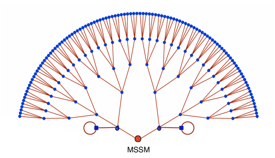
Figure 5: There is most likely a large landscape of UV gauge theories which connect via a duality cascade to the MSSM in the IR. Starting at the MSSM and proceeding up towards the UV, the duality cascade may encounter a succession of bifurcations which represent different possible sequences of Seiberg dualities. In this paper, we will identify two ways of connecting the MSSM to a special cascade which both follow regular periodic duality paths (as indicated by the two closed circles) rather than a chaotic sequence of dualities.

Starting from the MQSM, there are many ways in which this theory may connect to a duality cascade in the UV. Typically, these duality sequences are very irregular, and involve a succession of gauge theories with rapidly growing gauge group ranks and number of generations. The RG flow may even display a chaotic structure due to the fact that small variations in the relative size of gauge couplings may affect the order in which different quiver nodes undergo Seiberg dualities [40, 41]. As a result, a sequence of dualities will encounter multiple bifurcation points where a given ‘magnetic’ theory can connect to two or more different ‘electric’ theories. Our expectation is that there is likely a large landscape of UV theories which flow via a duality cascade to the MSSM in the IR. See figure 5 for a schematic depiction of this branching process. Rather than study a random cascade which may ‘accidentally’ connect to the MQSM, we shall instead focus on a minimal class of distinguished UV theories which exhibit a periodic duality cascade that terminates at the MQSM.  As a matter of notation, we shall denote a sequence of dualities as a string of labels indicating which node has been dualized.

4.1 Cascade Criteria

We now abstract from the above example of the Klebanov Strassler cascade to provide a stringent set of criteria which we shall require any candidate cascade which UV completes the MQSM to satisfy.  Due to the fact that we do not at present possess a string theory construction of the above cascade, we shall only consider cascades such that the resulting quiver theory has the maximal chance of possessing a candidate holographic dual.  As is evident in the example of the conifold, the appearance of a well-behaved holographic dual requires that all gauge group factors with finite gauge couplings must have a smooth large $N$ limit.  To reach the bottom of a more general cascade with low rank gauge groups, it therefore follows that each gauge group factor must dualize repeatedly over the course of the cascade.  We shall therefore require that in any candidate cascade:

• Each node with finite gauge coupling must possess a smooth large N limit.  As a consequence, each such node must dualize repeatedly during the cascade.

Whereas the ranks of the conifold theory continue to deplete during the entire cascade, the amount of bifundamental matter remains constant.  From the perspective of the associated intersection pairing, it follows that during the entire cascade the intersection pairing of the cycles wrapped by the branes remains constant.  On the other hand, it is well known that in more general geometric realizations of Seiberg duality in the context of type IIB brane probe theories, dualization corresponds to a flop within a Kähler cone.  When the quiver theory returns to its original connectivity, it implies that the geometry has returned to the original Kähler cone up to some monodromy at large radius.  While it is conceivable that a holographic dual may exist even when the intersection pairing of the branes does not return to the original connectivity of the quiver theory, it is reasonable to suppose that cascading brane configurations which repeatedly return to the same Kähler cone are most likely to possess a holographic dual description.  For this reason, we also require that in any candidate cascade:

• The number of bifundamentals must remain roughly constant over the span of the entire cascade.

Practical experience shows that this condition appears particularly difficult to satisfy for a generic chiral quiver gauge theory. Indeed, the above condition greatly restricts the number of available candidate cascades. While it is in principle possible to relax the criteria we propose, it is intriguing that even under these stringent conditions, the chiral matter content of the MQSM is arranged in such a way that the resulting candidate cascades satisfy the above criteria.

4.2 RG Node Locking

In addition to the above restrictions, we must also require that any proposed sequence of Seiberg dualities remains compatible with RG flow from the UV to the IR.  In particular, assuming that the Seiberg dual of any strongly coupled quiver node subsequently flows to weak coupling in the IR, the next stage of the cascade must dualize another node of the quiver theory.  We now argue that the presence of too much tensor matter can force a quiver node to flow to weak coupling.

At various stages of the covering theory cascade, bifundamental matter may appear between a node and its image under the orientifold action.  In the orientifold theory these bifundamentals descend to matter transforming in either the two index symmetric $(S)$, anti-symmetric $(A)$ or conjugate representations.  As will be explicit in all of the the cases studied below, the number of arrows between a quiver node and its image in the covering theory will always be either zero or at least $2g$.  These fields then descend to at least $g$ fields in the $S$ and $g$ in the $A$ representation of $U(N)$.  The one loop coefficient of the beta function of the non-abelian gauge coupling in the orientifold theory is therefore:

$$b_{SU(N)} =3N-\frac{\mbox{\small 1}}{\mbox{\small 2}}{\left(N+2\right)g}-\frac{\mbox{\small 1}}{\mbox{\small 2}}{\left(N-2\right)g}-F$$ (18)

$$=\left(3-g\right)N-F$$

where $F>0$ denotes all additional contributions from fields charged under the $SU(N)$ gauge group. The above argument is self-consistent because at weak coupling the one loop approximation to the running of the couplings should be an accurate description. Nevertheless, it is conceivable that contributions to the anomalous dimensions of fields can significantly alter the RG flow of coupling constants during a given cascade. The presence of such a large amount of tensor matter, however, implies that the effective number of flavors $F_{eff}$ will always be greater than $3N$ so that the above analysis should remain valid beyond the one loop approximation.  When $g\geq 3$, we therefore conclude that any quiver node with a sufficient amount of tensor matter will always flow to weak coupling.  As should now be evident, this severely restricts possible candidate cascade paths.

4.3 Connecting to the MQSM: Higgsing or Confinement

In this subsection we discuss the possible ways in which the gauge groups and matter content of the MQSM may appear at the bottom of a duality cascade.  Note that the field content of the MQSM alone cannot realize a cascade which satisfies the above stringent criteria.  Indeed, suppose to the contrary that a large $N$ generalization of the MQSM eventually cascades to the MQSM.  It follows at once from the above discussion of RG node locking that once the $USp$ factor at node $a$ dualizes, too much tensor matter will be present at the other nodes.  Hence, once the $USp$ factor dualizes to a weakly coupled description, all three gauge group factors will flow to weak coupling in the IR.  We therefore conclude that any candidate cascade which realizes the MQSM at the bottom of the cascade must contain at least four quiver nodes. We will label the three MQSM nodes by $a$, $b$, $c$, and the extra node by $d$.

There are in general two ways in which the MQSM can embed inside such a four node quiver.  Attaching an extra node to the MQSM, the most direct analogue of the Klebanov Strassler cascade corresponds to the case where the rank of the gauge group factor on the extra node depletes to zero at the bottom of the cascade.  Rather than requiring that the extra node confine at the bottom of the cascade, it is also possible to Higgs the quiver theory before the ranks of any node completely depletes so that two of the quiver nodes collapse to a single node, thereby reproducing the three node MQSM quiver.

In either scenario, any candidate single node extension of the MQSM must satisfy the requirements described in section 4.1.  Indeed, as will be evident from the discussion below, the qualitative requirement that the cascade repeat in an appropriate sense will impose tight restrictions on the connectivity of four node cascading quiver theories which eventually terminate at the MQSM.

5 Cascade in the Higgsing Scenario

In this section we discuss the cascade of a four node quiver theory which realizes the MQSM at the bottom of the cascade via the Higgsing scenario.  In order to satisfy the criteria of section 4.1, we require that the connectivity and number generations of the corresponding four node quiver remain stable throughout nearly all of the cascade.  We note that in the explicit example that we shall now consider, there is – besides the fact that it is needed for establishing a periodic cascade – an additional physical motivation for adding a fourth node to the MQSM: such an extension naturally restores left-right symmetry in the UV.

5.1 A Left-Right Symmetric Extension of the MQSM

Given that node $a$ of the MQSM quiver only couples to left-handed chiral matter, it is natural to identify the extra node $d$ with its right-handed partner. The $\mathbb{Z}_{2}$ symmetry that interchanges node $a$ and $d$ then becomes identified with left-right symmetry. To reduce the number of unknown parameters in the construction, we require that this left-right symmetry is restored further up the cascade.  The minimal quiver realization of a left-right model is shown in figure 6. As before, oriented lines represent $g=3$ generations of chiral matter. The dashed lines each represent a single vector pair of chiral superfields corresponding to the up/down Higgs pair of $USp(2)_{L}$ and $USp(2)_{R}$. Note that this LR model has no matter lines between node $b$ and $c$.

Figure 6: A minimal left-right symmetric extension of the MSSM (a). Each oriented line represents $g=3$ generations of chiral matter and each dashed line represents a single vector-like pair. Left-right symmetry breaking reproduces the matter content of the MQSM with three additional fields transforming in the adjoint of node $t$ (b). We interpret these additional fields as right-handed neutrinos.

We now briefly explain how to Higgs this model to the MQSM.  The LR quiver model has two $U(1)$ symmetries, of which only the combination:

$$\mathcal{Q}_{B-L}={\frac{1}{2}}(\mathcal{Q}_{U(1)_{c}}-\mathcal{Q}_{U(1)_{b}})$$ (19)

is non-anomalous. The other $U(1)$ symmetry has mixed anomalies, that we assume are cancelled via a Green-Schwarz mechanism of the type discussed in section 2.1. The same GS mechanism also produces a large mass for the abelian vector boson of the anomalous $U(1)$.

The right-handed quarks and leptons combine into $USp(2)_{R}$ doublets

$$Q_{R}=\left(\begin{array}[c]{c}U\\ D\end{array}\right),\qquad L_{R}=\left(\begin{array}[c]{c}N\\ E\end{array}\right)\,.$$ (20)

There is a vector pair of doublets $H_{3},H_{4}$, which are the right-handed mirrors of the MSSM Higgs. Left-right-symmetry is broken via the assumption that $H_{3},H_{4}$ both acquire a vev that is much larger than the electro-weak symmetry breaking scale

$$H_{3}=\left(\begin{array}[c]{c}a_{1}\\ a_{2}\end{array}\right)\,,\qquad H_{4}=\left(\begin{array}[c]{c}b_{1}\\ b_{2}\end{array}\right)\,.$$ (21)

We may use the $USp(2)_{R}$ symmetry to set $a_{2}=0$. The D-term constraints impose $b_{1}=0$ and $a_{1}=b_{2}$.  The most economical mechanism for generating this Higgs vev is to assume that the superpotential takes the form

$$W(H_{3},H_{4})=\mu_{R}(H_{3}H_{4}-{1\over 2a_{1}^{2}}(H_{3}H_{4})^{2}).$$ (22)

Minimizing $W$ allows for two supersymmetric minima, one of which breaks the left-right symmetry. The fields $H_{3}$ and $H_{4}$ are neutral under the $U(1)$ subgroup of $USp(2)_{R}\times U(1)_{b}$ generated by the linear combination

$$\mathcal{Q}_{U(1)_{t}}=\mathcal{Q}_{U(1)_{b}}+2\,T_{\!R}{}_{3}.$$ (23)

Thus the quiver nodes $b$ and $d$ collapse to a single node $t$, representing an anomalous $U(1)_{t}$ symmetry. The hypercharge symmetry $U(1)_{Y}$ is generated by the non-anomalous combination

$$Y={\frac{1}{2}}(\mathcal{Q}_{U(1)_{c}}-\mathcal{Q}_{U(1)_{t}})={}\mathcal{Q}_{{B-L}}-T_{\!R}{}_{3}.$$ (24)

The Higgsing of $USp(2)_{R}\times U(1)_{b}\rightarrow U(1)_{t}$ produces 3 massive gauge bosons with a mass of order the gauge coupling times $a_{1}$. We will denote this mass scale by $\Lambda_{LR}$. Traditionally the scale $\Lambda_{LR}$ is taken to be much larger than the electro-weak scale. Further discussion on the various energy scales in this left-right model appear in section 9. Of the original fields between the $U(1)$ and $USp(2)_{R}$ node, in the low energy theory we are left over with three right-handed lepton superfields $E$ and three sterile neutrinos denoted $N$. The effective theory far below the scale $\Lambda_{LR}$ is described by the MQSM quiver in figure 6b.

The Yukawa couplings in the MQSM descend from quartic superpotential terms in the unbroken LR theory. The same type of quartic couplings also give a contribution to the $\mu$-term $\lambda H_{u}H_{d}H_{3}H_{4}\rightarrow\lambda{a_{1}^{2}}H_{u}H_{d}$. To avoid a $\mu$-term that is too large, one needs to assume that the corresponding coupling $\lambda$ is small, or that this contribution is approximately cancelled via the ‘bare’ mu-term $\mu_{L}H_{u}H_{d}$. Reducing the complete quartic superpotential of the LR model, a priori also produces various undesirable $R$-parity violating couplings. However, these are easily eliminated if we require the LR superpotential to be invariant under a $\mathbb{Z}_{2}$ symmetry which acts as

$$R(Q)=R(L)=-1,\qquad R(H)=+1.$$ (25)

Where by abuse of notation, $R$ denotes the matter parity of a given superfield.

5.2 Left-Right Symmetric Duality Cascade

We now turn to describe the LR duality cascade. On general grounds, the LR model can be viewed as an orientifold of a quiver gauge theory. As shown in figure 7, the covering theory has the shape of an octahedron. As we will see in the next section, the cascading quiver that connects to the MQSM via the confining scenario will exhibit the same octahedral symmetry.  In order for holography to remain compatible with the orientifold projection, our expectation is that all cascades of the covering theory must descend in an appropriate fashion to the orientifold theory.

Consider the LR quiver gauge theory with general ranks as depicted in figure 7. First, suppose that node $b$ or $c$ reaches strong coupling first, and undergoes a Seiberg duality. The $b$ node has $2(g+2)N_{a}$ flavors, so the duality acts via

$$N_{b}\rightarrow 2(g+2)N_{a}-N_{b}\,.$$ (26)

Node $c$ has $2gN_{a}$ flavors, and its duality maps

$$N_{c}\rightarrow 2gN_{a}-N_{c}\,.$$ (27)

Since neither node has tensor matter, or connects to the other node, each Seiberg duality has a very simple action on the chiral matter content of the quiver. Each existing chiral line is reversed, indicating the replacement of quarks and leptons by dual quarks and leptons. The same is true for the vector lines, connecting nodes $b$ with nodes $a$ and $d$. There are extra mesons produced in each duality which connect nodes $a$ and $d$. But since $a$ and $d$ are $USp$ nodes, and as seen from the cover quiver, these mesons automatically come in vector pairs. Assuming generic quartic superpotential couplings, these mesons are all massive, and can be omitted from the low energy theory.

Next consider the case that node $a$ and/or $d$ reach strong coupling and dualize. For simplicity, we will mostly assume that left-right symmetry is completely restored during the UV part of the cascade, and that $a$ and $d$ have the same coupling. The two nodes then dualize simultaneously at the same scale. Each node has $gN_{c}+(g+2)N_{b}$ flavors, so that in the Seiberg dual theory the ranks change to:

$$2N_{a}\rightarrow gN_{c}+(g+2)N_{b}-2N_{a}-4.$$ (28)

Again, all matter lines reverse orientation in accord with their replacement by dual matter. While dual meson fields will also be created which connect nodes $b$ and $c$, the left-right symmetry of the Higgsing scenario implies that these fields come in vector-like pairs. We shall therefore assume that these acquire a mass due to quartic superpotential couplings in the UV theory. A more detailed analysis of how such mass terms arise in the context of the confining scenario cascade is given in Appendix B.

A priori, we could assume that $a$ and $d$ have different couplings and that the duality happens at different scales. As long as the two dualities happen in direct sequence, the above discussion remains unaltered. However, one could worry then that either node $b$ or $c$ would dualize at an energy scale between the energy scales where $a$ or $d$ dualizes. However, it is easy to see that this can not happen: whenever $a$ or $d$ dualizes, this creates extra tensor like matter for nodes $b$ and $c$, that prevents them from dualizing. This is the RG node locking mechanism discussed in section 4.2. In other words, the cascade can proceed only after both $a$ and $d$ have dualized, so that all tensor and chiral matter lines between $b$ and $c$ pair up and become massive. The Seiberg dualities proceed in an alternating sequence where the duality $(ad)$ is followed by duality map on nodes $b$ and/or $c$, and then again $(ad)$. It may happen that in between two $(ad)$ dualities, either both nodes $b$ and $c$ dualize or just one of the two. Since neither duality alters the connectivity of the quiver, the periodicity of the cascade is preserved either way.

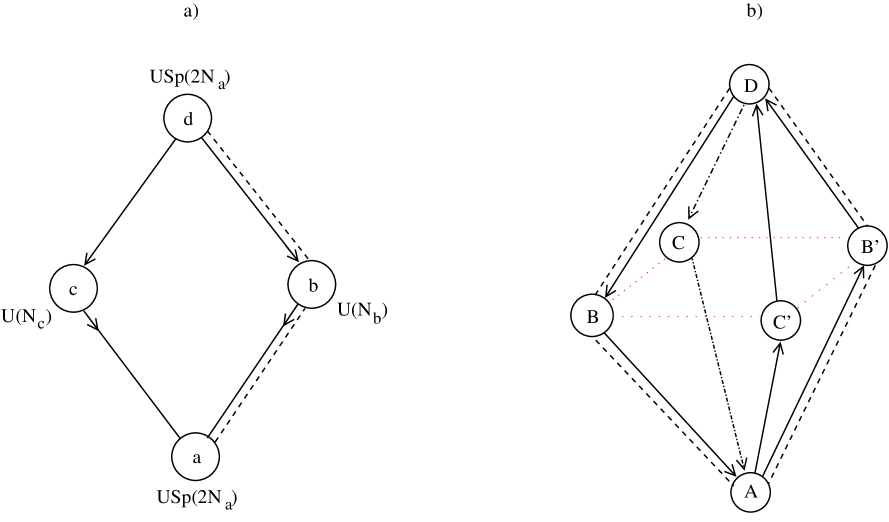
Figure 7: The left-right model with general gauge group ranks (a). Each oriented line indicates $g=3$ chiral matter fields, and the dashed lines each represent a single vector-like pair of Higgs fields. The covering theory (b) has the shape of an octahedron.

It is important to note that throughout this duality cascade, there are never any massive vector-like meson pairs created that connect nodes $a$ with $b$ or $c$, or node $d$ with $b$ or $c$. This is important for the following reason. Even if such meson pairs are massive, and thereby decouple from the low energy theory, they could still mix with the vector-like Higgs fields that connect node $b$ with nodes $a$ or $d$. This mixing would produce a large mass for the Higgs scalars, which would lift them from the low energy spectrum. Thus the absence of this class of meson pairs is an important fact, which helps secure the stability of the left-right quiver and preserve the presence of light Higgs scalars.

As a somewhat related point, we note that the superpotential obtained through Seiberg duality is always invariant under matter parity if the initial superpotential is, where matter parity acts as $\pm 1$ on a magnetic edge of the quiver if and only if it acts as $\pm 1$ on the dual electric edge. The reason is that the potential in the dual theory is of the schematic form $W\sim W_{\mathrm{micro}}+mxy$ where $x,y$ are dual quarks, and $m$ is a meson which inherits its parity from the electric theory. With our assignment of matter parity to $x$ and $y$, $m$ is even if and only if the product $xy$ is even. From this we conclude that the Seiberg dual superpotential is also invariant under matter parity.

This concludes our first description of the left-right symmetric cascade. In section 8 we will describe the IR region of the cascade, and how it connects with the MQSM.

6 Cascade in the Confining Scenario

The analysis of the previous section establishes that the MQSM can in principle lie at the bottom of a cascade which terminates by partially Higgsing a four node quiver.  In this section we begin our analysis of the other candidate scenario whereby a cascade terminates when the extra node confines.  As opposed to the relatively simple combinatorics of candidate cascades in the LR model, the combinatorics of the confining scenario requires a much longer sequence of steps before the resulting quiver returns to its original connectivity.

Because the classification of candidate cascades is more involved than in the LR cascade, we first provide a summary of the analysis to follow.  In order to classify candidate cascades in the orientifold theory, we study in Appendix A the admissible cascades of the covering theory which preserve the $\mathbb{Z}_{2}$ orientifold action and properly descend to the orientifold theory.  We note that while it is in principle possible to perform this field theoretic classification of cascades purely in the orientifold theory, in the context of holography it is important to establish that any candidate cascade correctly descend from the covering theory to its orientifold.

The combinatorics of the cascade significantly limit possible single node extensions of the covering theory.  Although we shall integrate out nearly all vector-like pairs generated by the cascade, we shall at first allow $n\geq 0$ massless vector-like Higgs pairs of bifundamentals connecting nodes $b$ and $a$.  It follows from the covering theory analogue of RG node locking discussed in section 4.2 that when a sufficient amount of chiral matter connects a quiver node to its image, the resulting pair of quiver nodes can never dualize.  In fact, when the extra node attaches to the MQSM by purely chiral matter, we find that all of the “locking matter” lifts if and only if the quiver theory has precisely one Higgs pair.  More generally, although we have not completely classified all possible ways in which vector-like matter can be added to a single node extension of the MQSM, we present some further examples where the extra node also attaches by vector-like matter to the MQSM.

6.1 Cascade Classification

In Appendix A we determine necessary conditions which any single node extension of the MQSM by purely chiral matter must satisfy in order to admit a periodically repeating cascade structure.  We begin this classification by studying cascades in the covering theory.  Assigning gauge group ranks compatible with the $\mathbb{Z}_{2}$ orientifold symmetry, we find that cancelling all non-abelian anomalies greatly restricts the ways in which the extra node can attach to the MQSM.  Restricting to this class of quiver topologies, we next consider candidate cascades in both the covering theory and its orientifold, and find that unless the arrows of the covering theory have multiplicity $g$, the cascade cannot proceed.  The end result of the classification argument as outlined in Appendix A is that only the second quiver in figure 8, denoted by $Q_{+}$, can give rise to a periodic cascade which descends to the orientifold theory denoted by $q_{+}$.  Moreover, this cascade properly descends only when $\alpha$, the number of bifundamentals that connect the extra node $D$ to nodes $B$, $B^{\prime}$, $C$ and $C^{\prime}$ equals the number of generations: $\alpha=g$.  The analysis of Appendix A also establishes that the cascade can only proceed when the gauge group factor of the extra node in the orientifold theory is of $USp$ type.

Figure 8: The quiver theories $Q_{-}$ and $Q_{+}$ correspond to the two distinct ways to attach a single additional node to the covering theory of the $g$ generation  MQSM by purely chiral matter.  The label $\alpha$ by each arrow indicates $\alpha$ bifundamentals.  All other oriented lines denote $g$ bifundamentals so that there are $2g$ arrows between $B^{\prime}$ and $B$. The dashed line denotes a vector-like pair and $n$ denotes the number of such pairs. In this section we show that only $Q_{+}$ supports a periodic cascade which descends to its orientifold when $\alpha=g$ and $n=1$.

6.2 Number of Higgs Pairs

The analysis of Appendix A demonstrates that there is at most one way to attach one additional node by purely chiral matter to the covering quiver of the MQSM so that the resulting quiver admits a cascade which properly descends to a repeating cascade in the orientifold theory.  We note that apart from the lines connecting $B$ and $B^{\prime}$ and the presence of additional vector-like matter, the connectivity of this quiver is identical to that of an octahedron.  In this section we show that the pair of nodes $BB^{\prime}$ can only dualize when the number of Higgs pairs is exactly one.  On the other hand, we also show that when only a subset of quiver nodes are dualized, the number of Higgs pairs in the orientifold theory is unconstrained.

A cascade in which all nodes are dualized at least once necessarily dualizes the pair corresponding to $B$ and $B^{\prime}$.  In order to simultaneously preserve the $\mathbb{Z}_{2}$ symmetry of the orientifold action while dualizing this pair, the number of bifundamentals connecting $B$ and $B^{\prime}$ must vanish.  Beginning with the quiver theory $Q_{+}$, we denote the dualized quiver by a string of letters indicating which nodes have dualized. A candidate cascade will lead to one of two candidate quiver theories $ADQ_{+}$ or $ADCC^{\prime}Q_{+}$.  See figure 9 for a depiction of these two quiver theories for general $n$.  In both cases, while the number of bifundamentals connecting $C$ and $C^{\prime}$ vanishes, the number connecting $B$ and $B^{\prime}$ is:

$$n_{BB^{\prime}}=2g(n-1)\text{.}$$ (29)

In order for the next stage of the cascade to dualize $B$ and $B^{\prime}$ it follows that $n=1$.  Assuming that neither cascade proceeds by this route, the next stage of the two cascades lead to the quiver theories $CC^{\prime}ADQ_{+}$ and $CC^{\prime}ADCC^{\prime}Q_{+}$ for $ADQ_{+}$ and $ADCC^{\prime}Q_{+}$, respectively.  We note, however, that although the amount of vector-like matter which must be integrated out depends on whether $n$ equals zero, in all cases the connectivity of the quiver $CC^{\prime}ADQ_{+}$ is identical to $ADCC^{\prime}Q_{+}$ and that of $CC^{\prime}ADCC^{\prime}Q_{+}$ to $ADQ_{+}$.  We therefore conclude that if the cascade never proceeds through the dualization of the pair $B$ and $B^{\prime}$, there are exactly four distinct connectivities for the quivers given by $Q_{+}$, $CC^{\prime}Q_{+}$, $ADQ_{+}$ and $ADCC^{\prime}Q_{+}$.  Because the number of bifundamentals connecting $B$ and $B^{\prime}$ is $2g$ for the first two theories and $2g(n-1)$ for the latter two, a cascade which dualizes the pair $B$ and $B^{\prime}$ can only proceed provided $n=1$.

To show that this result descends to the orientifold theory we return to lines (79) and (80) of Appendix A.  When $\alpha=g$ and $\varepsilon=-1$, the total amount of tensor matter at node $b$ vanishes when $n=1$.  A similar analysis holds for the other candidate paths.

Figure 9: Starting from the quiver theory $Q_{+}$ depicted in figure 8, the two candidate sequences of Seiberg dualities consistent with the $\mathbb{Z}_{2}$ action of the orientifold theory lead to the quiver theories $ADQ_{+}$ and $ADCC^{\prime}Q_{+}$.  In the figure, $\beta=g(n-1)$.  When $n=1$ all arrows in the common plane of $B,B^{\prime},C$ and $C^{\prime}$ vanish.

On the other hand, there is no restriction on $n$ when only the quiver nodes $A$, $D$, $C$ and $C^{\prime}$ participate in the cascade.  Indeed, tracing through the discussion given above, we find that such quiver theories also periodically repeat.  In fact, up to permutations in the order of dualization for the nodes $A$ and $D$, there are only two sequences of dualization consistent with the assumption that a dualized node subsequently flows to weak coupling.  The two possible sequences are given by alternately dualizing the pairs $CC^{\prime}$ and $AD$:

$$(CC^{\prime})(AD)(CC^{\prime})(AD)Q_{+} =Q_{+}$$

$$(AD)(CC^{\prime})(AD)(CC^{\prime})Q_{+} =Q_{+}$$ (30)

where a pair of dualizations enclosed by brackets commute.

In comparison with the covering theory of the LR cascade, we note that in the case of the quiver theory $Q_{+}$, there are now matter lines between nodes $B$ and $B^{\prime}$, as well as between $B$ and $C$.  Indeed, this additional connectivity is responsible for the far tighter restrictions on the matter content of the cascading quivers of the confining scenario.

Assuming that the number of Higgs pairs remains constant during the entire cascade, up to complex conjugation of some fields and interchanging the rôles of nodes $a$ and $d$, there are four types of quivers which can appear in the process of cascading down from $q_{+}$ (see figure 10).  As the above qualifications suggest, in section 6.4 we show that once the specific form of the superpotential is taken into account, the number of Higgs pairs can sometimes change as the cascade proceeds.  An example of this behavior is shown in figure 12 which demonstrates that the rôles of the $USp$ groups at nodes $a$ and $d$ can also interchange rôles as the cascade proceeds.

Figure 10: Up to re-orienting the directions of arrows or complex conjugating tensor matter representations, when the Higgs pair remains exactly massless, there are four types of quiver theories which can arise from a cascade which begins with the quiver theory $q_{+}$.  Unless otherwise indicated, each oriented line denotes $g=3$ bifundamentals.  The dashed line denotes a single Higgs-up/Higgs-down pair.  A similar classification into four quiver types also holds for more general values of $g$.

6.3 More General Vector-Like Matter

It is intriguing that in its minimal form, the single node extension by purely chiral matter requires precisely one Higgs pair in order for other stages of the cascade to proceed.  For more general single node extensions, however, there may also be a number of additional massless vector-like pairs present.  Letting $v_{GH}$ denote the number of vector-like pairs between a pair of nodes $G$ and $H$, if we assume that all other vector-like pairs develop a mass and can be integrated out, a similar cascade will proceed when the number of added vector-like pairs obey the conditions:

$$n =v_{AB}=v_{AB^{\prime}}=v_{DB}+1=v_{DB^{\prime}}+1$$

$$m =v_{DC}=v_{DC^{\prime}}=v_{AC}=v_{AC^{\prime}}$$ (31)

$$p =v_{BC}=v_{B^{\prime}C^{\prime}}=v_{BC^{\prime}}=v_{B^{\prime}C}\text{.}$$

In section 8 we shall consider one such extension which serves to accelerate the first stage of dualization in proceeding from the IR to the UV.  To simplify some of the analysis to follow, in the rest of this section we shall restrict to the case of the single node extension by purely chiral matter.

Figure 11: Depiction of the single node extension of the cover of the MQSM which attaches by both chiral matter and vector-like pairs.  Each oriented line denotes $g$ bifundamentals.  Vector-like pairs are denoted by dashed lines with the multiplicity indicated.

6.4 Superpotential Analysis

The analysis of the previous sections establishes that at the level of the matter content and connectivity of the quiver theory, a periodic cascading structure may occur in the confining scenario provided all vector-like pairs except for the Higgs pair lift at each intermediate stage.  To demonstrate that this is indeed realized, in Appendix B we classify all candidate terms in the superpotential of a given electric theory which could potentially produce a quadratic term in the superpotential of the dual magnetic theory.  Due to the fact that quadratic terms in the magnetic theory can sometimes appear as composite cubic or quartic operators in the original electric theory variables, we first present the most general form of the superpotential up to quartic order in the quiver fields.  It is a consequence of the topology of the quiver theory that at nearly all stages of the cascade the dual magnetic theory contains a mass term for all vector-like matter except for the Higgs pair.  In fact, we find that there is only a single stage of the cascade where a candidate mass term for the Higgs pair can develop.

In order to classify all possible mass terms in the dual magnetic theory obtained during each stage of the cascade, it is sufficient to determine all admissible gauge invariant terms up to quartic order for the quiver theories obtained at intermediate stages of the cascade process.  To this end, we now argue that it is enough to only treat the quiver theories of type $a)$ and $d)$ in figure 10.  Because nodes $b$ and $c$ cannot dualize when tensor matter is present, nodes $a$ and $d$ always dualize together.  Further, because nodes $a$ and $d$ do not share any bifundamental matter, the number of vector-like pairs attached to either node cannot disappear by dualizing $a$ or $d$.  This implies that the dual superpotential given by dualizing the pair $a$ and $d$ is also independent of the order in which the cascade proceeds.  Because dualizing nodes $c$ and $b$ does not introduce any chiral matter and only reverses the orientation of quiver arrows, it is therefore enough to determine the form of the dual superpotential for quivers of type $a)$ and $d)$ in figure 10.

As shown in Appendix B, whereas generically all other vector-like pairs will develop a mass at some stage of the cascade, there is only one possible candidate quiver topology which upon dualizing produces a mass term for the previously massless Higgs pair.

With notation as defined in Appendix B, in the electric theory corresponding to the quiver theory $q_{+}$, the superpotential contains the terms:

$$W_{q_{+}}\supset\lambda_{ij}X_{ca}^{i}X_{a\overline{b}}X_{b\overline{c}}^{j}+\widehat{\lambda}_{ij}^{I}X_{ca}^{i}X_{ab}^{I}X_{\overline{bc}}^{j}+\varphi_{ijkl}X_{ac}^{i}X_{\overline{cb}}^{j}X_{b\overline{c^{\prime}}}^{k}X_{c^{\prime}a}^{l}\text{.}$$ (32)

In addition to the original vector-like Higgs pair between nodes $a$ and $b$, dualizing node $c$ will produce $g^{2}$ additional vector-like pairs corresponding to new meson fields.  Letting $C$ denote the mesons created by dualizing node $c$, the magnetic dual superpotential of the quiver theory $cq_{+}$ contains terms of the form:

$$W_{c(q_{+})}\supset\left[\begin{array}[c]{cc}X_{\overline{b}a}&C_{\overline{b}a}^{kl}\end{array}\right]_{1\times\left(g^{2}+1\right)}\left[\begin{array}[c]{cc}\mu_{I}&\mu_{c}\lambda_{ij}\\ \mu_{c}\widehat{\lambda}_{kl}^{I}&\mu_{c}^{2}\varphi_{klij}\end{array}\right]_{(g^{2}+1)\times\left(g^{2}+g+1\right)}\left[\begin{array}[c]{c}X_{ab}^{I}\\ C_{ab}^{ij}\end{array}\right]_{\left(g^{2}+g+1\right)\times 1}$$ (33)

where the fields $C$ denote meson fields created by dualizing node $c$.  For generic values of the couplings, precisely $g$ chiral fields charged in the fundamental of $b$ and $a$ will remain and all vector-like pairs will develop a mass.

6.4.1 R-parity

Although the above analysis demonstrates that in most cases the resulting vector-like pairs develop a mass, generic values for the couplings produce phenomenologically undesirable interaction terms.  Returning to standard MSSM notation, these include terms of the form:

$$\mu_{i}X_{a\overline{b}}X_{ba}^{i} =\mu_{i}H_{u}L^{i}$$

$$\widehat{\lambda}_{ij}^{k}X_{ca}^{i}X_{ab}^{k}X_{\overline{bc}}^{j} =\widehat{\lambda}_{ij}^{k}Q^{i}L^{k}D^{j}$$ (34)

which lead to lepton number violating interactions.  To prevent such terms, it is customary to require that the Lagrangian density remain invariant under R-parity. As already discussed in the context of the Higgsing scenario, this is compatible with our cascade structure. This also applies to the confining scenario. Nevertheless, for the benefit of the reader we will discuss the R-parity assignments in the confining cascade scenario in more detail here.  In a Lorentz invariant theory, this is equivalent to assigning a matter parity of $(-1)^{3(B-L)}$ to each superfield of the theory.  This has the effect of splitting the $g+1$ bifundamentals:

$$X_{ba}^{I}\rightarrow X_{ba}^{0}\oplus X_{ba}^{i}\text{.}$$ (35)

Due to the fact that this parity assignment corresponds to a real subgroup of a $U(1)$ group, the matter parity of a field remains the same after Seiberg dualizing a quiver node.  All composite operators such as meson fields therefore also inherit a definite matter parity.  Returning to the quiver theory $q_{+}$, the matter parity of the fields are:

$$\ \ \qquad\qquad R(X_{[\overline{bb^{\prime}}]}^{i})=\alpha_{i}$$

$$R(X_{ca}^{i},X_{\overline{bc}}^{i},X_{b\overline{c}}^{i},X_{ba}^{i},X_{(\overline{bb^{\prime}})}^{i})=-1$$

$$\ \ \qquad\qquad R\left(X_{d\overline{c}}^{i}\right)=\beta_{i}$$ (36)

$$R\left(X_{ab}^{0},X_{a\overline{b}}\right)=+1$$

$$\ \ \qquad\qquad R\left(X_{d\overline{b}}^{i}\right)=\gamma_{j}\text{.}$$

Scanning through the possible terms of Appendix B, we find that when $\alpha_{i}=-1$ and $\beta_{i}=\gamma_{j}$ for all $i$, $j$, the vector-like pairs of fields studied in the previous section still develop quadratic terms in the superpotential of the dual magnetic theory.  This has the consequence that one of the chiral fields attached to node $d$ has non-trivial lepton number.  We shall return to the matter parity of the additional fields in section 6.5.

Although imposing matter parity does reduce the number of allowed superpotential terms, it does not resolve the problem encountered in equation (33).  Indeed, the corresponding quadratic term for the dual meson fields now takes the form:

$$R\left(W_{c(q_{+})}\right)\supset\left[\begin{array}[c]{cc}X_{\overline{b}a}&C_{\overline{b}a}^{kl}\end{array}\right]_{1\times\left(g^{2}+1\right)}\left[\begin{array}[c]{cc}\mu_{0}&\mu_{c}\lambda_{ij}\\ \mu_{c}\widehat{\lambda}_{kl}^{0}&\mu_{c}^{2}\left(\varphi_{klij}+\widehat{\varphi}_{ijkl}\right)\end{array}\right]_{(g^{2}+1)\times\left(g^{2}+1\right)}\left[\begin{array}[c]{c}X_{ab}^{0}\\ C_{ab}^{ij}\end{array}\right]_{\left(g^{2}+1\right)\times 1}$$ (37)

where in the above we have used the fact that the $C^{ij}$ have matter parity $+1$.  Note that although the fields $X_{ab}^{i}$ no longer appear in the corresponding term and are therefore massless, the remaining vector-like matter between nodes $a$ and $b$ will still generically develop a mass.

6.5 The Cascading $\mu$ problem and Higgs Regeneration

As shown in the previous section, although generic values of the couplings in the orientifold theory lead to mass terms for most vector-like pairs, at nearly all stages of the cascade the Higgs pair remains exactly massless.  Even so, dualizing node $c$ in the quiver theory $q_{+}$ will generate a $(g^{2}+1)\times(g^{2}+1)$ mass matrix with rank $g^{2}+1$.  Such a mass matrix will lift all vector-like pairs between nodes $a$ and $b$.  On the other hand, due to the fact that node $b$ can only dualize when no tensor matter is present, it follows from the analysis near equation (29) that in order to lift the tensor matter present at node $b$, the cascade must retain a single nearly massless Higgs pair.  Once this pair develops a mass, the results of the previous section establish that while the cascade can still proceed by dualizing all nodes other than $b$, the rank of $b$ will remain constant throughout the rest of the cascade.

While the above arguments hold for generic values of the couplings, relations between couplings in the covering theory can sometimes descend to non-trivial restrictions on the form of the superpotential in the orientifold theory.  In this section we show that while the Higgs pair may disappear from the massless spectrum at intermediate stages of the cascade, when the couplings $\varphi_{ijkl}$ of equation (32) correspond to a $g^{2}\times g^{2}$ matrix of rank $g^{2}-1$, a new Higgs pair will automatically regenerate further down the cascade.  After presenting a general analysis of how the cascade proceeds as the Higgs pair disappears and regenerates, we present an explicit realization of this mechanism where the octahedral symmetry of the covering theory naturally enforces the condition that the matrix $\varphi_{ijkl}$ is anti-symmetric.  In this case we find that the rank of the matrix is generically $g^{2}-1$ only when $g$ is an odd number.

6.5.1 Higgs Regeneration

Assuming that all other couplings remain sufficiently generic so that all other vector-like pairs develop a mass, we now show that when the couplings $\varphi_{ijkl}$ of equation (32) correspond to a $g^{2}\times g^{2}$ matrix of rank $g^{2}-1$, the Higgs pair between nodes $a$ and $b$ regenerates further down the cascade.  For simplicity, we restrict our discussion to matter parity invariant superpotentials.  Starting from the quiver theory $q_{+}$, consider the dualized theory $cq_{+}$.  It follows from equation (37) that even when $\varphi_{ijkl}$ has rank $g^{2}-1$, the corresponding quadratic form will still be non-degenerate.  In this case, all vector-like pairs between nodes $a$ and $b$ lift, leaving only $g$ oriented lines corresponding to the lepton doublets.  Due to the fact that node $b$ still flows to weak coupling in the IR, the next stage of the cascade must proceed by dualizing the pair of nodes $a$ and $d$.  Note that whereas all tensor matter created at node $c$ lifts as before, the number of arrows attached between node $b$ and $d$ is now equal to the number between $b$ and $a$.  Because these two sets of arrows have opposite orientation, all tensor matter at node $b$ created by dualizing $a$ and $d$ will generically develop a mass and lift from the massless spectrum.  Because similar reasoning applies to the tensor matter produced at node $c$, it follows that the next stage of the cascade must proceed by dualizing node $c$.

In comparison to the original quiver theory $q_{+}$, the quiver theory $adcq_{+}$ does not possess any vector-like pairs.  Note in particular that the rôles of nodes $a$ and $d$ have also interchanged.  Indeed, upon dualizing node $c$, the orientation of lines attached to node $c$ dictate that no vector-like pairs appear between nodes $a$ and $b$.  Instead, precisely $g^{2}$ vector-like pairs develop between nodes $d$ and $b$.  Assuming that the matter parity of the superfields $X_{d\overline{c}}^{i}$ and $X_{db}^{i}$ is equal to that of the lepton doublets between nodes $a$ and $b$, it follows that the quiver theory $adcq_{+}$ contains the terms:

$$W_{adcq_{+}}\supset\chi_{ijkl}X_{d\overline{c}}^{i}X_{c\overline{b}}^{j}X_{bc^{\prime}}^{k}X_{\overline{c^{\prime}}d}^{l}\text{.}$$ (38)

The couplings $\chi_{ijkl}$ are the analogue of the couplings $\varphi_{ijkl}$ in the quiver theory $q_{+}$.  Indeed, upon dualizing node $c$, $\chi_{ijkl}$ corresponds to a $g^{2}\times g^{2}$ quadratic form in the magnetic dual superpotential.  Due to the exchange of rôles for nodes $a$ and $d$, first suppose that whatever considerations require the matrix $\varphi_{ijkl}$ to have rank $g^{2}-1$ also apply to the matrix $\chi_{ijkl}$.  In this case, the resulting quadratic terms in the superpotential of the dual magnetic theory $cadcq_{+}$ cause all but one vector-like pair of fields between nodes $d$ and $b$ to develop a mass.  Because nodes $a$ and $d$ have simply exchanged rôles in the cascade, we therefore conclude that the cascade will proceed as before.  Indeed, at the next stage, dualizing the pair of nodes $a$ and $d$ now generically lifts the tensor matter present at node $b$ so that node $b$ is free to dualize.  Iterating through the cascade once more, it follows that eventually the cascade will return to a quiver theory similar to $q_{+}$ where the next step of the cascade dualizes node $c$.  Reversing the rôles of the matrices of couplings $\varphi_{ijkl}$ and $\chi_{ijkl}$, in the next cycle the vector-like matter between nodes $d$ and $b$ generically develops a mass, but a new massless vector-like pair regenerates between nodes $a$ and $b$.  See figure 12 for a sequence of dualities which exhibits the disappearance and regeneration of the Higgs pair when $\varphi$ and $\chi$ both have rank $g^{2}-1$.  In order for nodes $a$ and $d$ to exchange rôles at intermediate stages of the cascade, the matter attached to node $a$ must also exchange rôles with the matter attached to node $d$.

Figure 12: Starting from the quiver theory $q_{+}$, dualizing node $c$ introduces a generic $g^{2}\times g^{2}$ mass term for all vector-like matter between nodes $a$ and $b$.  As shown in the rightmost figure, further down the cascade a Higgs pair will regenerate between nodes $d$ and $b$ when the mass matrix for the dual meson fields has rank $g^{2}-1$.

Alternatively, even when the matrix of couplings $\chi_{ijkl}$ is generic, the rank constraint on $\varphi_{ijkl}$ will still regenerate a massless Higgs pair between nodes $a$ and $b$.  Although dualizing node $c$ of the quiver theory $adcq_{+}$ in this case produces $g^{2}$ vector-like pairs between nodes $d$ and $b$ which generically develop a mass, the subsequent dualization of nodes $a$ and $d$ results in the quiver theory $adcadcq_{+}$.  But the topology of this quiver is identical to that of the quiver $q_{+}$ with the vector-like pair between nodes $a$ and $b$ deleted.  It now follows by similar reasoning that dualizing node $c$ regenerates a massless vector-like pair of fields between nodes $a$ and $b$.

Although originally introduced simply to make the cascade proceed, regenerating the Higgs pair naturally decouples the $\mu$-term from any candidate UV completion of the field theory.  In the sense that generically the $\mu$-term is expected to be sensitive to Planck scale physics, we can claim to have partially solved the $\mu$ problem.

6.5.2 Reflection Symmetry and Path Rules

The argument of the previous section establishes that when an appropriate symmetry reduces the ranks of the matrices of couplings $\varphi_{ijkl}$ and $\chi_{ijkl}$ to $g^{2}-1$, the cascade regenerates the single massless Higgs pair necessary for other stages of the cascade to proceed.  Although it is possible to simply impose a relation on the couplings at some stage of the cascade, unless this rule derives from a symmetry of some kind, we must explicitly check that this same symmetry persists further down the cascade.  For this reason, we now present an explicit symmetry which reduces the rank of the corresponding coupling matrix.  While it is in principle possible to impose an explicit discrete symmetry of the flavor group $U(3)^{5}$ which reduces the rank of the matrices of couplings, an arbitrary choice would likely obscure the underlying geometry of a candidate compactification. To this end, we now show that there exists a symmetry of the covering quiver theory such that the matrices of couplings $\varphi_{ijkl}$ and $\chi_{ijkl}$ will be anti-symmetric. When $g$ is an odd number, the corresponding matrices will have rank $g^{2}-1$.

Because we expect on general grounds that explicit automorphisms of the quiver theory will naturally lift to conditions on the geometry probed by a stack of D-branes, we restrict our analysis to automorphisms of the quiver theory which interchange the rôles of the quiver nodes. The automorphisms of the covering theory $Q_{+}$ are generated by two $\mathbb{Z}_{2}$ generators $r$ and $R$, where $r$ denotes reflection about the plane cut by the nodes $A$, $D$, $B$ and $B^{\prime}$ and $R$ denotes rotation by an angle of $\pi$ about the axis passing through the nodes $A$ and $D$.  More precisely, the reflection fixes the bifundamentals $X_{B^{\prime}\overline{B}}^{i}$, $X_{B\overline{A}}^{i}$ and $X_{A\overline{B^{\prime}}}^{i}$ and interchanges all other fields in the obvious fashion.  In order for the action of matter parity to remain compatible with the reflection symmetry, at other stages of the cascade we shall require that all additional meson fields between $B^{\prime}$ and $B$ remain fixed by the reflection symmetry and that all additional vector-like pairs of fields between $B$ and $A$ or $B^{\prime}$ and $A$ interchange with a counterpart.  Whereas the $\mathbb{Z}_{2}$ identification of quiver nodes of the orientifold theory corresponds to identification by the rotation group symmetry, the reflection $r$ does not descend from the quiver $Q_{+}$ to $q_{+}$.  Indeed, from the perspective of the orientifold theory the symmetry $r$ interchanges fields transforming in different representations of the same gauge group.

Because each piecewise connected path maps to an operator, it is enough to study the action of $r$ on the algebra of paths with two or more links.  We now show that there exists a representation of the $\mathbb{Z}_{2}$ action $r$ on the algebra of paths in the quiver theory which imposes the desired anti-symmetry condition on the matrices of couplings $\varphi_{ijkl}$ and $\chi_{ijkl}$ while leaving all other couplings sufficiently generic to lift all remaining vector-like pairs.  In order to fully specify the action of the reflection symmetry on the algebra of paths in the covering theory $Q_{+}$ we shall not require that the starting and ending point of a given path be the same.  We claim that a consistent action on the path algebra of each quiver theory encountered during the cascade is given by the rules:

• Path Rule 1: Although invariance under some other symmetry may impose additional relations on the couplings, no further restriction is imposed on the coupling constant matrices corresponding to paths which do not map to a connected path in the image.

• Path Rule 2: A path/operator with a connected image path which passes $n$ times perpendicularly through the plane of reflection maps to the image path/operator weighted by $(-1)^{n}$.

In the above, paths which pass perpendicularly through the plane of reflection are defined as paths which contain a directed or anti-directed (e.g. with all arrows reversed) subpath of one of the following types:

$$\{C\rightarrow A\rightarrow C^{\prime},C^{\prime}\rightarrow A\rightarrow C,C\rightarrow C^{\prime},C^{\prime}\rightarrow C,C\rightarrow D\rightarrow C^{\prime},C^{\prime}\rightarrow D\rightarrow C\}\text{.}$$ (39)

The first rule is a necessary condition for a consistent action on the algebra of paths due to the fact that some gauge invariant paths do not always map to gauge invariant paths under the action of $r$.  For example, letting $\Lambda$ denote an index which runs from $1$ to $2g$, the closed path $C\rightarrow A\rightarrow B^{\prime}\rightarrow B\rightarrow C$ corresponding to the operator $\tau_{ij}^{I\Lambda}X_{C\overline{A}}^{i}X_{A\overline{B^{\prime}}}^{I}X_{B^{\prime}\overline{B}}^{\Lambda}X_{B\overline{C}}^{j}$ in the quiver $Q_{plus}$ does not map to a gauge invariant counterpart.  Because all meson fields created during the cascade respect the reflection symmetry of the octahedron, the above rules remain intact during each stage of the cascade.

Invariance under the action of the reflection symmetry imposes the desired relation on the matrix of couplings $\varphi_{ijkl}$.  Indeed, under the reflection symmetry, the path $C\rightarrow A\rightarrow C^{\prime}\rightarrow B\rightarrow C$ corresponding to the operator $\varphi_{ijkl}X_{C\overline{A}}^{i}X_{A\overline{C^{\prime}}}^{j}X_{C^{\prime}\overline{B}}^{k}X_{B\overline{C}}^{l}$ maps to:

$$r\left(\varphi_{ijkl}X_{C\overline{A}}^{i}X_{A\overline{C^{\prime}}}^{j}X_{C^{\prime}\overline{B}}^{k}X_{B\overline{C}}^{l}\right) =-\varphi_{ijkl}X_{C\overline{A}}^{j}X_{A\overline{C^{\prime}}}^{i}X_{C^{\prime}\overline{B}}^{l}X_{B\overline{C}}^{k}$$ (40)

$$=-\varphi_{jilk}X_{C\overline{A}}^{i}X_{A\overline{C^{\prime}}}^{j}X_{C^{\prime}\overline{B}}^{k}X_{B\overline{C}}^{l}$$

so that invariance of the path implies $\varphi$ is anti-symmetric.

In order to demonstrate that the above symmetry allows the cascade to proceed, it is enough to show that the relations on all other couplings are sufficiently mild so as to leave the rest of the cascade intact.  Because a similar analysis can be applied for the quiver theory $CC^{\prime}Q_{+}$, it is enough to treat the relations among couplings in the quiver theories $Q_{+}$ and $ADQ_{+}$. Including all possible terms up to quartic order, the most general superpotential of the quiver theory $Q_{+}$ is:

$$W_{Q_{+}} =\mu_{I}X_{B\overline{A}}^{I}X_{A\overline{B}}+\mu_{I}^{\prime}X_{A\overline{B^{\prime}}}^{I}X_{B^{\prime}\overline{A}}+\lambda_{ij}X_{C\overline{A}}^{i}X_{A\overline{B}}X_{B\overline{C}}^{j}+\lambda_{ij}^{\prime}X_{A\overline{C^{\prime}}}^{i}X_{C^{\prime}\overline{B^{\prime}}}X_{B^{\prime}\overline{A}}^{j}$$

$$+\widehat{\lambda}_{ij}^{I}X_{C\overline{A}}^{i}X_{A\overline{B^{\prime}}}^{I}X_{B^{\prime}\overline{C}}^{j}+\widehat{\lambda}_{ij}^{\prime I}X_{C\overline{A}}^{i}X_{A\overline{B^{\prime}}}^{I}X_{B^{\prime}\overline{C}}^{j}+\sigma_{\Lambda}^{IJ}X_{A\overline{B^{\prime}}}^{I}X_{B^{\prime}\overline{B}}^{\Lambda}X_{B\overline{A}}^{J}$$

$$+\alpha_{ijkl}X_{D\overline{C}}^{i}X_{C\overline{A}}^{j}X_{A\overline{C^{\prime}}}^{k}X_{C^{\prime}\overline{D}}^{l}+\gamma_{ij}^{IJ}X_{D\overline{B}}^{i}X_{B\overline{A}}^{I}X_{A\overline{B^{\prime}}}^{J}X_{B^{\prime}\overline{D}}^{j}$$

$$+\tau_{ij}^{I\Lambda}X_{C\overline{A}}^{i}X_{A\overline{B^{\prime}}}^{I}X_{B^{\prime}\overline{B}}^{\Lambda}X_{B\overline{C}}^{j}+\tau_{ij}^{\prime I\Lambda}X_{A\overline{C^{\prime}}}^{i}X_{C^{\prime}\overline{B^{\prime}}}^{j}X_{B^{\prime}\overline{B}}^{\Lambda}X_{B\overline{A}}^{I}$$

$$+\beta_{ijk}^{I}X_{D\overline{C}}^{i}X_{C\overline{A}}^{j}X_{A\overline{B^{\prime}}}^{I}X_{B^{\prime}\overline{D}}^{k}+\beta_{ijk}^{\prime I}X_{C^{\prime}\overline{D}}^{i}X_{D\overline{B}}^{j}X_{B\overline{A}}^{I}X_{A\overline{C^{\prime}}}^{k}$$

$$+\varphi_{ijkl}X_{C\overline{A}}^{i}X_{A\overline{C^{\prime}}}^{j}X_{C^{\prime}\overline{B}}^{k}X_{B\overline{C}}^{l}+\varphi_{ijkl}^{\prime}X_{C\overline{A}}^{i}X_{A\overline{C^{\prime}}}^{j}X_{C^{\prime}\overline{B^{\prime}}}^{k}X_{B^{\prime}\overline{C}}^{l}$$ (41)

$$+\mu_{IJ}^{(1)}(X_{B^{\prime}\overline{A}}X_{A\overline{B^{\prime}}}^{I})(X_{B^{\prime}\overline{A}}X_{A\overline{B^{\prime}}}^{J})+\mu_{IJ}^{(2)}(X_{A\overline{B}}X_{B\overline{A}}^{I})(X_{A\overline{B}}X_{B\overline{A}}^{J})$$

$$+\mu_{IJ}^{(3)}(X_{A\overline{B}}X_{B\overline{A}}^{I})(X_{B^{\prime}\overline{A}}X_{A\overline{B^{\prime}}}^{J})+\kappa_{IJ}^{(1)}X_{B_{1}^{\prime}\overline{A_{1}}}X_{A_{1}\overline{B_{2}^{\prime}}}^{I}X_{B_{2}^{\prime}\overline{A_{2}}}X_{A_{2}\overline{B_{1}^{\prime}}}^{I}$$

$$+\kappa_{IJ}^{(2)}X_{A_{1}\overline{B_{1}}}X_{B\overline{{}_{1}A_{2}}}^{I}X_{A_{2}\overline{B_{2}}}X_{B\overline{{}_{2}A_{1}}}^{I}+\widehat{\kappa}_{IJ}X_{B\overline{A}}^{I}X_{A\overline{B^{\prime}}}^{J}X_{B^{\prime}\overline{A}}X_{A\overline{B}}\text{.}$$

Invariance under reflection symmetry imposes the following relations on these couplings:

$$\qquad\ \ \qquad\alpha_{ijkl}=\alpha_{lkji}$$

$$\lambda_{ij}=\widehat{\lambda}_{ij}^{\prime 0}$$

$$\qquad\ \ \qquad\varphi_{ijkl}=-\varphi_{jilk}$$ (42)

$$\lambda_{ij}^{\prime}=\widehat{\lambda}_{ij}^{0}$$

$$\qquad\ \ \qquad\varphi_{ijkl}^{\prime}=-\varphi_{jilk}^{\prime}$$

which descend to the superpotential $W_{q_{+}}$ of the orientifold theory given by equation (86).  We note that this symmetry requires that the Yukawa couplings of the up and down type quarks are exactly equal at each intermediate stage of the cascade.  In other words, the CKM matrix of the resulting theory is diagonal.  Presumably suitably small off diagonal components develop near the bottom of the cascade. The observed hierarchy $m_{top}\gg m_{bottom}$ in this scenario must arise from a proportional hierarchy between the Higgs up and down expectation values.

Similarly, the most general superpotential of the quiver theory $ADQ_{+}$ is:

$$W_{ADQ_{+}} =\mu_{I}X_{B\overline{A}}^{I}X_{A\overline{B}}+\mu_{I}^{\prime}X_{A\overline{B^{\prime}}}^{I}X_{B^{\prime}\overline{A}}$$

$$+\alpha_{ijkl}X_{C\overline{D}}^{i}X_{D\overline{C^{\prime}}}^{j}X_{C^{\prime}\overline{A}}^{k}X_{A\overline{C}}^{l}+\gamma_{ij}^{IJ}X_{B\overline{D}}^{i}X_{D\overline{B^{\prime}}}^{j}X_{B^{\prime}\overline{A}}^{I}X_{A\overline{B}}^{J}$$

$$+\beta_{ijk}^{I}X_{C\overline{D}}^{i}X_{D\overline{B^{\prime}}}^{j}X_{B^{\prime}\overline{A}}^{I}X_{A\overline{C}}^{k}+\beta_{ijk}^{\prime I}X_{D\overline{C^{\prime}}}^{i}X_{C^{\prime}\overline{A}}^{j}X_{A\overline{B}}^{I}X_{B\overline{D}}^{k}$$ (43)

$$+\mu_{IJ}^{(1)}(X_{B^{\prime}\overline{A}}X_{A\overline{B^{\prime}}}^{I})(X_{B^{\prime}\overline{A}}X_{A\overline{B^{\prime}}}^{J})+\mu_{IJ}^{(2)}(X_{A\overline{B}}X_{B\overline{A}}^{I})(X_{A\overline{B}}X_{B\overline{A}}^{J})$$

$$+\mu_{IJ}^{(3)}(X_{A\overline{B}}X_{B\overline{A}}^{I})(X_{B^{\prime}\overline{A}}X_{A\overline{B^{\prime}}}^{J})+\kappa_{IJ}^{(1)}X_{B_{1}^{\prime}\overline{A_{1}}}X_{A_{1}\overline{B_{2}^{\prime}}}^{I}X_{B_{2}^{\prime}\overline{A_{2}}}X_{A_{2}\overline{B_{1}^{\prime}}}^{I}$$

$$+\kappa_{IJ}^{(2)}X_{A_{1}\overline{B_{1}}}X_{B\overline{{}_{1}A_{2}}}^{I}X_{A_{2}\overline{B_{2}}}X_{B\overline{{}_{2}A_{1}}}^{I}+\widehat{\kappa}_{IJ}X_{B\overline{A}}^{I}X_{A\overline{B^{\prime}}}^{J}X_{B^{\prime}\overline{A}}X_{A\overline{B}}\text{.}$$

Invariance under the path condition now requires that the $g^{2}\times g^{2}$ matrix of couplings $\alpha_{ijkl}$ must be symmetric.

Figure 13: Depiction of the sequence of Seiberg dualities leading from $q_{+}$ to $adbcadq_{+}$.  At the next stage of the cascade, node $c$ dualizes which generically eliminates the Higgs pair from the quiver theory.

6.6 Candidate Cascade Sequences

As argued previously, there is an essentially unique way to extend the MQSM by a single node so that a cascade can always proceed.  Even so, the distinct sequence of Seiberg dualities adopted by a candidate cascade will in general depend on the initial values of the ranks and coupling constants in the UV.  Moreover, while many candidate cascades will eventually repeat back to the quiver theory $q_{+}$, there are in principle sequences which can fail to return to the quiver theory $q_{+}$.  To classify possible cascades, note that whenever node $c$ dualizes when it is attached to node $b$, it will either generate or destroy a Higgs pair in the corresponding quiver.  Letting $c_{+}$ and $c_{-}$ denote dualizations which respectively create or destroy such a pair, we note that $c_{+}$ and $c_{-}$ always appear together in the combination:

$$I\equiv(ad)c_{+}(ad)c_{-}$$ (44)

where as before, a pair of dualizations enclosed by brackets commute.  Beginning from the quiver theory $q_{+}$, any candidate sequence of cascades is necessarily of the form:

$$S_{1} \equiv\cdot\cdot\cdot G_{n}^{(i_{n})}\cdot\cdot\cdot IG_{2}^{(i_{2})}IG_{1}^{(i_{1})}q_{+}$$

$$S_{2} \equiv\cdot\cdot\cdot G_{n}^{(i_{n})}\cdot\cdot\cdot G_{2}^{(i_{2})}IG_{1}^{(i_{1})}Iq_{+}$$

where each $G_{n}^{(i_{n})}$ corresponds to one of three possible intermediate sequences:

$$G_{n}^{(1)} =(ad)b$$

$$G_{n}^{(2)} =(ad)c$$ (45)

$$G_{n}^{(3)} =(ad)(bc)\text{.}$$

In order for a subsequence of $I$’s and $G_{i}$’s to eventually repeat back to $q_{+}$, its conjugate with all arrow directions reversed, or a quiver theory with the rôles of $a$ and $d$ interchanged, nodes $b$ and $c$ must attach to node $a$ with the same orientation.  A similar statement holds for connections to node $d$.  Due to the fact that each $I$ and $G^{(3)}$ subsequence preserves the relative orientation of nodes $b$ and $c$ in terms of how they attach to nodes $a$ and $d$, only $G^{(1)}$ and $G^{(2)}$ can change this relative orientation.  We therefore conclude that a sequence of dualities will only repeat back to $q_{+}$ or a quiver theory whose connectivity is physically indistinguishable when the total number of number of $G^{(1)}$ and $G^{(2)}$ dualities is even.  To summarize, a sequence beginning at $q_{+}$ will or will not repeat back to $q_{+}$ or a physically indistinguishable quiver theory when:

Repeat: $$\#G^{(1)}+\#G^{(2)}\in 2\mathbb{Z}$$

Not Repeat $$\text{: }\#G^{(1)}+\#G^{(2)}\notin 2\mathbb{Z}\text{.}$$

This is essentially a consequence of the fact that dualizing node $c$ in $q_{+}$ destroys the Higgs pair.  Indeed, assuming the superpotential has been sufficiently tuned so that dualizing node $c$ does not change the number of Higgs pairs, it is possible to show that the cascade always eventually repeats.  With this in mind, note that although a given sequence may not return to the quiver theory $q_{+}$, up to the presence of a single Higgs pair, a similar analysis establishes that the chiral matter content always eventually repeats.

We now consider candidate cascade sequences with additional vector-like pairs present. As will be shown in more detail in section 8.2.1, the observed values of the couplings imply that additional vector-like pairs must in fact be added in order for the cascade to begin dualizing at sub-Planck scales. Assuming that all other additional vector-like pairs are always integrated out, the cascade can proceed when an equal number of vector-like pairs attach nodes $a$ to $c$ and $c$ to $d$. We now show that when the number of vector-like pairs is an even number, this addition will not disrupt the Higgs regeneration mechanism described previously. To this end, consider dualizing node $c$ of the quiver theory $q_{+}$ with the Higgs pair deleted. The number of vector-like pairs of mesons created now yields $(m+g)g$ pairs between nodes $a$ and $b$ and $mg$ pairs between nodes $d$ and $b$. In order for the Higgs regeneration mechanism to proceed as before, we must treat the extra vector-like pairs in a similar fashion to the other bifundamentals between nodes $a$ and $c$. Further, the mechanism can only work when $(m+g)g$ is an odd number so that $g$ is odd and $m$ is even. Indeed, because $mg$ is an even number, a generic meson mass matrix will lift all pairs between nodes $d$ and $b$ and leave a single pair between $a$ and $b$. When $m$ is an odd number, the same mechanism would create a vector-like pair between nodes $d$ and $b$ instead of between nodes $a$ and $b$. Next dualizing nodes $a$ and $d$, the number of bifundamentals between nodes $b$ and $c$ will now double. This has the consequence that all subsequent dualizations of node $c$ will always produce an even number of vector-like pairs between nodes $a$ and $b$ and between nodes $d$ and $b$. We therefore conclude that $m$ must be an even number in order for the Higgs regeneration mechanism to remain intact.

7 Ultraviolet Unification of Higgsing and Confining Scenarios

Although in comparison with the rather intricate cascade combinatorics of the confining scenario, there is an essentially unique path of dualization for the Higgsing scenario.  At intermediate stages, however, the quiver topology of the confining scenario is nearly identical to that of the Higgsing scenario.  Indeed, the only difference between the quiver of the LR cascade with a single Higgs pair and the quiver theory $adq_{+}$ is that the LR model has one additional vector-like pair connecting nodes $d$ and $b$. We now explain how the two scenarios unify in the UV of the cascade.

Figure 14: An intermediate stage of the cascade for the covering quiver in the confining (a) and Higgsing (b) scenarios.  These two scenarios unify at higher energy.  Indeed, the only difference between the two quivers is the presence (b) or absence (a) of an extra vector-like pair (dashed line).

To this end, note that introducing a $\mu$ term for one of the two vector-like pairs of the LR model would break the $\mathbb{Z}_{2}$ symmetry of the model.  Nevertheless, a cascading structure will remain intact, although the MQSM will now arise via the confining scenario.  Conversely, when an ostensibly massive vector-like pair which would normally be integrated out survives as an anomalously light vector-like pair in the quiver theory $adq_{+}$, the resulting cascade will now proceed via a LR cascade which connects to the MQSM at the bottom of the cascade via the Higgsing scenario.

8 The Bottom of the Cascade

In both the Higgsing and confining scenarios, the last steps of the cascade are in general different from the other intermediate stages due to the difference in the form of the dual superpotential when a gauge group confines.  Indeed, just prior to the final step where the four node quiver theory of the Higgsing scenario transitions to a three node quiver, the Higgsing scenario contains a $U(1)$ factor at node $b$.  From the perspective of the duality cascade, the non-abelian factor at node $b$ has confined without breaking chiral symmetry.  In the purely confining scenario, the ranks of the non-abelian factors at nodes $d$ and $b$ have both depleted to zero.  This implies that both gauge group factors have confined.  In this section we describe in further detail how the form of the superpotential of the MQSM arises from the last few duality steps realized at the bottom of the cascade. We also comment on how the extra node $d$ may play a rôle in initiating supersymmetry breaking at the bottom of the cascade.

8.1 Higgsing Scenario

The duality cascade described in section 5 reduces in the infrared to a supersymmetric, but otherwise minimal, left-right symmetric extension of the Standard Model with left-right gauge group $USp(2)_{L}\times USp(2)_{R}\simeq SU(2)_{L}\times SU(2)_{R}$. The phenomenology of such left-right symmetric models has been quite extensively studied in the literature [42, 43, 44, 45, 46]. It is beyond the scope of this paper to elaborate on the phenomenological strengths and weaknesses of this class of scenarios. To this end, we shall limit our discussion to scenarios where the bottom of the cascade realizes a phenomenological LR symmetric model. In this discussion, we start in the IR and work our way up towards the UV. To set the stage, we start with the left-right model itself and how its superpotential connects with that of the MQSM. We then proceed to discuss the first two duality cycles.

8.1.1 Left-Right Symmetry Breaking

We now discuss how the superpotential of the LR quiver in figure 6a descends to the superpotential of the MQSM quiver indicated in figure 6b. The left-right quiver theory has the form of a diamond, with oriented lines corresponding to the quarks and leptons, and two unoriented lines corresponding to the Higgs fields that will break the left-right and electro-weak symmetry. Left-right symmetry breaking may occur when the superpotential for the Higgs scalars $H_{3},H_{4}$ connecting nodes $b$ and $d$ takes the form given by equation (22). In one supersymmetric minimum of the corresponding effective potential, the extra Higgs fields attain the vacuum expectation values:

$$H_{3}=\left(\begin{array}[]{c}a_{1}\\ 0\\ \end{array}\right)\,,\qquad H_{4}=\left(\begin{array}[]{c}0\\ a_{1}\\ \end{array}\right).$$ (46)

Thus 3 gauge bosons eat 3 chiral fields and obtain a mass of order

$$\Lambda_{LR}\equiv g_{U(1)_{b}}\,a_{1}.$$ (47)

We are also left with an extra singlet field $S$ corresponding to changing $H_{3},H_{4}$ in the direction of the vev. Because the left-right symmetric quiver contains no oriented triangles, only quadratic and quartic terms appear to lowest order:

$$W_{LR} = \mu_{L}\,H_{u}H_{d}+\mu_{R}\,H_{3}H_{4}$$

$$+A_{IJKL}\,Q^{I}Q^{J}Q^{K}Q^{L}+B_{IJ}{}^{kl}\,Q^{I}Q^{J}X_{k}X_{l}+C^{ijkl}\,X_{i}X_{j}X_{k}X_{l}+\mathcal{O}_{6}.$$

In the above, $\mathcal{O}_{6}$ denotes all degree six and higher gauge invariant combinations of fields and $X$ is a collective label for $L$ or $H$, the fields that are charged under node $b$. We will discuss in the next subsection how the LR cascade generates this superpotential. An important point in this regard is that all couplings in $W_{LR}$ are dimensionful. This implies that all of their values are expected to be set by the common the mass scale $\Lambda_{1}$ of the first step up the cascade. As we will see, to generate an appropriate seesaw mechanism, the scale $\Lambda_{1}$ needs to be quite high – above $10^{11}$ TeV or so.

The MQSM superpotential follows by replacing $H_{3},H_{4}$ by its vev. The Yukawa couplings arise from the quartic terms

$$\begin{matrix}Q_{L}Q_{R}H_{3}H_{d}&\to&a_{1}Q_{L}DH_{d},\qquad&L_{L}L_{R}H_{3}H_{d}&\to&a_{1}L_{L}EH_{d}\\[5.69054pt] Q_{L}Q_{R}H_{u}H_{4}&\to&{a_{1}}Q_{L}UH_{u},\qquad&L_{L}L_{R}H_{u}H_{4}&\to&{a_{1}}L_{L}NH_{u}\end{matrix}$$

These Yukawa couplings are naturally of the right overall magnitude, provided the scale $\Lambda_{LR}$ of left-right symmetry breaking is sufficiently close to the scale $\Lambda_{1}$ set by the first Seiberg duality up the cascade. To reproduce the correct mass spectrum for all the Standard Model particles, the superpotential of the left-right model must accommodate the required mass hierarchy. Here we will not address whether this is a natural requirement, except to note that the model naturally includes a Majorana mass term for the sterile neutrinos

$$L_{R}H_{4}L_{R}H_{4}\rightarrow a_{1}^{2}N_{R}N_{R}\,.$$

Thus if we choose a high scale for $\Lambda_{LR}$, the theory automatically incorporates a seesaw mechanism. Further we get a second contribution to the $\mu$-term:

$$H_{u}H_{d}H_{3}H_{4}\to{a_{1}^{2}}\,H_{u}H_{d}\,.$$

In the context of this LR model, the $\mu$ problem is the question why this contribution cancels to such a large degree of accuracy with $\mu_{L}$.

The superpotential is restricted to be invariant under the matter parity assignments $R(Q)=R(L)=-1,\ R(H)=+1$. This invariance forbids the following operators

$$\begin{matrix}Q_{L}Q_{R}H_{3}L_{L}&\to&a_{1}\,Q_{L}DL_{L}\qquad\qquad\qquad&L_{L}L_{R}H_{3}L_{L}&\to&a_{1}\,L_{L}EL_{L}\\[5.69054pt] L_{L}H_{3}H_{u}H_{4}&\to&{a_{1}^{2}}\,L_{L}H_{u}\qquad\quad\qquad&H_{u}H_{d}L_{R}H_{4}&\to&{a_{1}}\,H_{u}H_{d}N\\[5.69054pt] \end{matrix}$$

which confirms that the matter parity of the LR model directly descends to the usual matter parity of the MSSM. For more details on the phenomenology of the LR model, we refer to the standard literature on this subject.

8.1.2 The First Duality: (De)Confinement of Node $b$

In this subsection we discuss the relation between the superpotential in the LR quiver and the superpotential in the first step up the cascade. The cascade terminates (towards the IR) when the $SU(9)$ gauge group on node $b$ confines at a scale $\Lambda_{1}$. Node $b$ has $N_{F}=10$, and therefore if $N_{c}=9$, it confines without chiral symmetry breaking. The quiver at this step is as shown in figure 7 with $(2N_{a},N_{b},N_{c})=(2,9,3)$. The gauge coupling for the $SU(9)_{b}$ is a priori unrelated to that of $U(1)_{b}$, and the scale $\Lambda_{1}$ is therefore a free parameter in the cascade. As we will see shortly, it is natural to chose $\Lambda_{1}$ slightly above the scale $\Lambda_{LR}$ where the left-right symmetry gets restored. We will refer to the theory above the scale $\Lambda_{1}$ as the electric theory, and to the one below $\Lambda_{1}$ as the magnetic theory.

In the electric theory, we denote the fields charged under node $d$ by $Q$ and the fields charged under node $b$ by $l,h$. We impose invariance under the matter parity transformation $R(Q)=R(l)=-1$ and $R(h)=+1$. Via the duality and LR symmetry breaking, this descends to the standard matter parity of the MQSM. The superpotential up to quartic terms is of the schematic form

$$W = \kappa_{L}\,h_{u}h_{d}+\kappa_{R}\,h_{3}h_{4}$$

$$+\alpha_{IJKL}\,Q^{I}Q^{J}Q^{K}Q^{L}+\beta_{IJkl}\,Q^{I}Q^{J}\mathrm{x}^{k}\mathrm{x}^{l}+\gamma_{ijkl}\,\mathrm{x}^{i}\mathrm{x}^{j}\mathrm{x}^{k}\mathrm{x}^{l}$$

where $\mathrm{x}$ is a collective label for the fields charged under node $b$, that is $l$ or $h$. The quartic couplings are of order $1/M_{2}$, where $M_{2}$ will later be related to scales higher up in the cascade. Around the scale $\Lambda_{1}$, the $SU(9)$ gauge sector confines and we must replace the superpotential (8.1.2) by its magnetic dual. The chiral fields in the dual theory are given by

$$m^{ij}=\mathrm{x}^{i}\mathrm{x}^{j}\,,\qquad\qquad X_{i}={\frac{1}{\Lambda_{1}^{N_{c}-1}}}\;\epsilon_{ij_{1}\ldots j_{N_{c}}}\mathrm{x}^{j_{1}}\ldots\mathrm{x}^{j_{N_{c}}}.$$ (50)

The dual baryons are the fields of the left-right symmetric theory discussed in the previous subsection. The dual mesons are additional vector-like matter. We did not consider the mesons as part of the low energy theory, because for generic superpotential, they acquire a high scale mass and need to be integrated out to obtain the low energy superpotential.

For $N_{f}=N_{c}+1$, the magnetic superpotential is generally given by

$$W={\frac{1}{\Lambda_{1}}}m^{i{j}}X_{i}{X}_{{j}}\;-{\frac{1}{\Lambda_{1}^{2N_{c}-1}}}\det(m).$$ (51)

Because the group $USp(2)_{L}\times USp(2)_{R}$ embeds in the $SU(N_{f})\times SU(N_{f})$ flavor group, the expression $\det(m)$ is gauge invariant and makes sense. This $\det(m)$ term in the superpotential is of higher order, and irrelevant for the low energy dynamics of the magnetic model when the anomalous dimensions of the dual meson fields are suitably small. The electric superpotential (8.1.2) thus descends to the following magnetic superpotential

$$W = \kappa_{L}\,m_{ud}+\kappa_{R}\,m_{34}$$

$$+\ \alpha_{IJKL}\,Q^{I}Q^{J}Q^{K}Q^{L}+\beta_{IJkl}\,Q^{I}Q^{J}m^{kl}+\gamma_{ijkl}\,m^{ij}m^{kl}+{\frac{1}{\Lambda_{1}}}\,m^{ij}X_{i}X_{j}.$$

It is clear that with generic quartic terms in the electric theory, we can lift all the mesons. Assuming a Kähler potential $K\sim m\bar{m}/\Lambda_{1}^{2}$, the masses of the mesons are of order $\Lambda_{1}^{2}/M_{2}$. We assume that this mass is large compared to $\Lambda_{LR}$. We can then safely integrate out the mesons to get the effective Lagrangian for the LR model. In this way, one obtains the superpotential as given in equation (8.1.1) where

$$A_{IJKL}=\alpha_{IJKL}+\beta_{IJkl}\beta_{klmn}\gamma^{klmn}\,,\qquad$$

$$\ \mu_{L}=\gamma^{udud}\frac{\kappa_{L}}{\Lambda_{1}}+\gamma^{ud34}\frac{\kappa_{R}}{\Lambda_{1}}$$

$$B_{IJ}{}^{kl}={\frac{1}{\Lambda_{1}}}\,\beta_{\operatorname{Im}Jn}\gamma^{mnkl}\qquad\qquad\qquad\ \$$

$$\ \mu_{R}=\gamma^{34ud}\frac{\kappa_{L}}{\Lambda_{1}}+\gamma^{3434}\frac{\kappa_{R}}{\Lambda_{1}}$$

$$C^{ijkl}=\;{\frac{1}{\Lambda_{1}^{2}}}\,\gamma^{ijkl}\,.\qquad\qquad\ \ \ \qquad\qquad$$

8.1.3 Second Step: Dualizing Nodes $a$ and $d$

We now to the relation between the superpotentials before and after the second step up the cascade.  In the theory above the scale $\Lambda_{1}$, the two $USp(2)$ nodes $a$ and $d$ have a total of $54$ flavors. This large number implies that both nodes acquire a large $\beta$ function and hit strong coupling at a scale $\Lambda_{2}$ that is just a couple of orders of magnitude larger than $\Lambda_{1}$. In the next section we shall provide approximate values for these energy scales. At the strong coupling scale $\Lambda_{2}$, both nodes $a$ and $d$ undergo a Seiberg duality. Since we assume that left-right symmetry is restored, the two nodes dualize simultaneously. In fact, the presence of additional tensor matter will greatly accelerate the running of the $b$ and $c$ nodes so that nodes $a$ and $d$ must dualize at very similar scales so that the theory does not prematurely reach a Landau pole at a quiver node with tensor matter. We shall return to this point in section 9.2. The theory above $\Lambda_{2}$ is the new electric theory. Its quiver diagram is as shown in figure 7, with $(2N_{a},N_{b},N_{c})=(48,9,3)$. The theory valid between $\Lambda_{2}$ and $\Lambda_{1}$ (the previous electric theory) now becomes the new magnetic theory, describing the effective dynamics of the dual quarks produced by the confinement transition of the two $USp(48)$ gauge factors. The electric superpotential is of the form

$$W=\lambda_{L}\,Z_{3}Z_{4}+\lambda_{R}\,Z_{u}Z_{d}+a^{IJKL}\,Y_{I}Y_{J}Y_{K}Y_{L}+b^{ijkl}\,Z_{i}Z_{j}Z_{k}Z_{l}+c^{IJkl}\,Y_{I}Y_{J}Z_{k}Z_{l}$$ (54)

where fields charged under node $c$ are denoted as $Y$ and fields charged under node $b$ are denoted as $Z$. Under matter parity, the vector-like fields $Z_{3},Z_{4},Z_{u},Z_{d}$ have charge $+1$ and all other fields have charge $-1$. The scale of the couplings $a,b,c$ is of order $1/M_{3}$ with $M_{3}$ the scale determined by the physics of the next duality step up in the cascade.

The Seiberg duality comes with an extra new scale m, that is not determined by the scale $\Lambda_{el}=\Lambda_{2}$ where the electric theory becomes strongly coupled. This scale m is related to the magnetic strong coupling scale $\Lambda_{mag}$ that influences the way the superpotential feeds through the duality. The magnetic superpotential is of the form

$$W = \lambda_{L}\,z_{ud}+\lambda_{R}\,z_{34}+a^{IJKL}\,y_{IJ}y_{KL}+b^{ijkl}\,z_{ij}z_{kl}+c^{IJkl}\,w_{Jk}w_{Li}$$ (55)

$$+\frac{1}{\mathrm{m}}\,y_{ij}Q^{i}Q^{j}+\frac{1}{\mathrm{m}}\,z_{ij}\mathrm{x}^{i}\mathrm{x}^{j}+\frac{1}{\mathrm{m}}\,w_{Ij}Q^{I}\mathrm{x}^{j}+\frac{1}{\mathrm{m}}\,w_{iJ}\mathrm{x}^{i}Q^{J}$$

The mesons are defined as

$$y_{IJ}=Y_{I}Y_{J},\quad z_{ij}=Z_{i}Z_{j},\quad w_{Ij}=Y_{I}Z_{j},\quad w_{iJ}=Z_{i}Y_{J}.$$ (56)

The mesons have a mass of order $\mathrm{m}^{2}/M_{3}$. Integrating them out yields the superpotential given in (8.1.2) where

$$\alpha_{IJKL}=\frac{a_{IJKL}}{\mathrm{m}^{2}}\qquad$$

$$\qquad\kappa_{L}=b_{udud}\frac{\lambda_{L}}{\mathrm{m}}+b_{ud34}\frac{\lambda_{R}}{\mathrm{m}}$$

$$\beta_{IJkl}=\frac{c_{IJkl}}{\mathrm{m}^{2}}\ \qquad$$

$$\qquad\kappa_{R}=b_{34ud}\frac{\lambda_{L}}{\mathrm{m}}+b_{3434}\frac{\lambda_{R}}{\mathrm{m}}$$

$$\gamma_{ijkl}=\frac{b_{ijkl}}{\mathrm{m}^{2}}.\ \qquad$$

These formulas summarize the matching relations at the second duality step. Combined with the matching rules (8.1.2) at the first duality step and the formulas of left-right symmetry breaking, they prescribe how the coefficients in the original superpotential (54) descend to various couplings of the MQSM. It would be worthwhile to investigate this dictionary in more detail. Undoubtedly one will find that the theory will need to satsify some stringent constraints. Whether or not these constraints can be satisfied with reasonable UV initial conditions will determine whether this LR cascade scenario has a chance of being phenomenologically viable.

8.2 Confining Scenario

Whereas the combinatorics of the intermediate stages of the confining scenario are more intricate than those of the Higgsing scenario, the analysis near the bottom of the cascade is comparatively less involved. Indeed, because the end of the cascade terminates when nodes b and d confine, it is only necessary to analyze the contributions to the superpotential from terms specific to when a given gauge group confines. Because each factor must confine without breaking chiral symmetry, the form of the superpotential will contain terms schematically of the form $BM\bar{B}-detM_{b}$ for node $b$ and $PfM_{d}$ for node $d$ where the subscript on $M$ denotes a generic meson field associated with a given gauge group and $B$ denotes a baryon operator. In these expressions, the number of generations and the non-zero rank of the neighboring flavor groups imply that these terms are of very high degree in comparison to the higher order quartic terms which we have retained in order to analyze how vector-like pairs develop a mass. Assuming that the cascade soon enters a regime where the above operators are not dangerous irrelevant, we may ignore their contribution to the low energy dynamics of the cascading theory. At higher stages of the cascade dualizing nodes $b$ and $d$ would produce additional cubic terms in the superpotential. These terms do not contribute to the mass terms necessary for lifting vector-like pairs of mesons created when nodes $c$ and $a$ dualize for the last time.

8.2.1 Igniting the Confining Scenario

Proceeding from the IR to the UV, the above analysis demonstrates that in the Higgsing scenario the energy scale at which the duality cascade begins can be arranged to lie below the Planck scale.  In the most minimal version of the confining scenario, where the extra node $d$ attaches to the MQSM by purely chiral matter, the first few stages of dualization are already far beyond the Planck scale.  To establish this, consider the first stage of dualization from the IR to the UV.  In the confining scenario, this corresponds to dualizing node $d$ at some energy scale $\Lambda_{d}$.  As argued previously, the unique next step must be the dualization of node $a$.  Note, however, that because there is no matter connecting nodes $a$ and $d$, to one loop order the running of the coupling at node $a$ is identical to that of the MSSM.  Because the running of the weak coupling of the MSSM only becomes strongly coupled at energy scales far above the Planck scale, we conclude that as the energy scale increases, gravitational effects will dominate before node $a$ dualizes.

In order to lower the first scale of dualization for node $a$, the running of the couplings must accelerate as the theory proceeds to higher energy scales.  In general, this will occur when extra matter has been added to node $a$.  It is not possible to add this matter in an arbitrary fashion, however, because at higher energy scales the cascade must still exhibit a periodic repeating structure.

We find that there are in fact many ways to accelerate the running of couplings so that the cascade ignites at sub-Planck scales.  In this section we present some examples of how this acceleration can be achieved by adding extra vector-like pairs which can be treated as additional massless degrees of freedom at sufficiently high energy scales.

Although the cascade requires that each node with finite gauge coupling must dualize repeatedly during the cascade, no such restriction holds for flavor groups with arbitrarily weak gauge coupling.  Indeed, a possible way to accelerate the cascade corresponds to adding one additional node to the quiver theory which attaches to node $a$ by some number of vector-like pairs.  In order to preserve the repeating structure of the cascade after node $a$ dualizes, node $d$ must connect to the extra node in exactly the same fashion as node $a$.  We note that because the nodes with $U$ type group factors still cannot dualize with tensor matter present, nodes $a$ and $d$ must dualize sequentially.  This implies that the combinatorics of the cascade proceed as before.

In principle, the presence of an extra node runs counter to the minimality of the cascade.  As explained in section 6.3, a very similar cascading structure exists when extra vector-like matter has been added symmetrically to the quiver theory.  A general concern in this context is that an extra vector-like pair must not develop a mass and lift as the cascade proceeds.  Consider for simplicity the cascade with $m$ vector-like pairs attached between nodes $d$ and $c$ and nodes $a$ and $c$.  To establish that such pairs will not develop a mass as the cascade proceeds, first recall that the Higgs pair generically lifted from the low energy spectrum because the presence of additional meson fields between nodes $b$ and $a$ (or $d$ and $b$) mixed sufficiently with the Higgs so that all vector-like pairs generically lifted from the resulting low energy spectrum.  In contrast, at no stage of the cascade do additional vector-like pairs ever appear between nodes $d$ and $c$ or between $a$ and $c$.  It now follows that as opposed to the Higgs pairs, there is no stage of the cascade which can produce a mass term for the vector-like pairs.  Finally, in order to maintain the Higgs regeneration mechanism discussed in section 6.5 , we must also preserve the condition that the anti-symmetric matrix $\varphi$ of equation (32) continues to have an odd number of rows and columns.  As explained in section 6.6, this requires that the number of additional vector-like pairs must be an even number.

8.3 Supersymmetry Breaking at the Bottom of the Cascade

In this brief section we discuss how supersymmetry breaking could in principle occur in the context of either the Higgsing or confining scenario.  Because a supersymmetric spectrum appears necessary for much of the cascade to proceed, it is natural to expect that supersymmetry breaking must occur at a scale below the last dualization.  As we have seen above, a cascade can only proceed when at least one additional node has been added to the MQSM.  In principle, it is possible to imagine that supersymmetry breaking also takes place at this extra node and only communicates to the rest of the particles of the MQSM through some higher order loop effects.  This would be the case, for example, in direct gauge mediation models [47, 48, 49].  In the present context such a realization will typically be phenomenologically unviable.  Indeed, in both the Higgsing and confining scenarios, the extra quiver node only attaches indirectly to the $SU(2)_{L}$ weak sector.  At the level of gaugino masses this would effectively produce a large mass splitting between the gluino and gluons, while producing an essentially supersymmetric spectrum for the $W$ bosons and winos.

Although it lies beyond the scope of the present paper, it is in principle possible that supersymmetry breaking may occur due to the cascade landing in a metastable non-supersymmetric vacuum.  Indeed, in many cases such vacua exist when a small mass term has been added to some subset of vector-like matter [50].  We note that such a scenario would naturally accommodate the proposed method to ignite the confining scenario cascade by adding extra vector-like matter.  Further, whereas the metastable vacua of [50] preserved R-symmetry and therefore did not allow the gauginos to develop a mass, generic higher dimension operators will always be present for the cascade to proceed.  As noted in [51], such generic quartic terms can deform the ISS vacuum to an R-symmetry breaking configuration where gaugino masses are now possible.

9 Energy Scales

9.1 Energy Scales of the Left-Right Cascade

The analysis of the previous section demonstrates that compatibility with the Standard Model imposes expectedly stringent boundary conditions on the IR region of the cascade. In this section we study the behavior of the cascade at higher energy scales. In flowing up the cascade, the ranks of the gauge groups increase very fast. For example, after just five duality steps, the ranks are $(2N_{a},N_{b},N_{c})=(48,231,141)$ and after six steps they are $(1526,231,141)$. This growth triggers an accelerated sequence of duality steps, that accumulate over an ever shorter range of scale, and the system quickly hits a duality wall. The duality wall should appear below the Planck scale. Indeed, the duality wall may be quite close to the Planck scale but can also be much lower in energy. The former option would provide a natural explanation for generating appropriate neutrino masses via a seesaw mechanism, whereas the latter option is of course more exciting in the context of potential observations at the LHC. At any rate, we have no a priori reason to prefer either choice of energy scale. For concreteness in the discussion to follow, we shall assume that this duality wall arises close to the string scale or Planck scale. For definiteness, let us assume the wall is placed at $10^{15}$ TeV. This UV boundary condition essentially determines the energy scales at which all the lower duality steps take place. We now give a rough estimate of these scales.

To obtain the scale dependence of the various couplings along the duality cascade, it does not suffice to use the perturbative formulas. The exact beta function of an ${\cal N}=1$ supersymmetric gauge theory with gauge group $G$ reads

$$\beta = \frac{d(4\pi/g^{2})}{d\log\mu}\,=\,\frac{3T(G)-\sum_{i}T(r_{i})(1-\gamma_{i})}{2\pi(1-\frac{g^{2}}{8\pi^{2}}T(G))}$$ (58)

where the sum runs over all matter multiplets, and $\gamma_{i}$ denotes their anomalous dimensions. Here $T(G)=3N$ for $SU(N)$ and $3(N+1)$ for $USp(2N)$, and $T(r)=1/2$ for matter in the (anti-)fundamental representation. The contribution from the anomalous dimensions and from the non-trivial denominator in (58) can be substantial.

Because we are only interested in a rough estimate of how fast the duality cascade accelerates in the UV, we shall approximate the above formula by $\beta=b_{0}/2\pi$ with $b_{0}=3N-N_{f}$ for $SU(N)$ with $N_{f}$ flavors and $b_{0}=3(N+1)-N_{f}/2$ for $USp(2N_{c})$ with $N_{f}$ flavors. Using this estimate, we find that the beta function of node $a$ and $d$ above the scale $\Lambda_{1}$ is of order $21/2\pi\sim 3.3$. Assuming that inverse coupling constant $\alpha_{a}^{-1}=4\pi/g_{a}^{2}$ at the scale $\Lambda_{1}$ is approximately 25, the second duality takes place at a scale $\Lambda_{2}$ that is around 3 orders of magnitude larger than $\Lambda_{1}$. A similar estimate shows that the next scale $\Lambda_{3}$, where node $b$ again reaches strong coupling, is at most one order of magnitude above $\Lambda_{2}$. The duality wall appears just a little above the scale $\Lambda_{3}$. In order for the wall to occur at around $10^{15}$ TeV, we thus find that the scale $\Lambda_{1}$ must be close to $10^{11}$ TeV or so. The next scale $\Lambda_{2}$ is then around $10^{14}$ TeV and all other steps take place in the string regime. Since the left-right symmetry breaking scale needs to be not too far below the first duality scale $\Lambda_{1}$, we conclude that a reasonable value for $\Lambda_{LR}$ is around $10^{10}$ TeV. A schematic plot of the running of the three non-abelian gauge couplings over the first five duality stages is shown in figure 15.

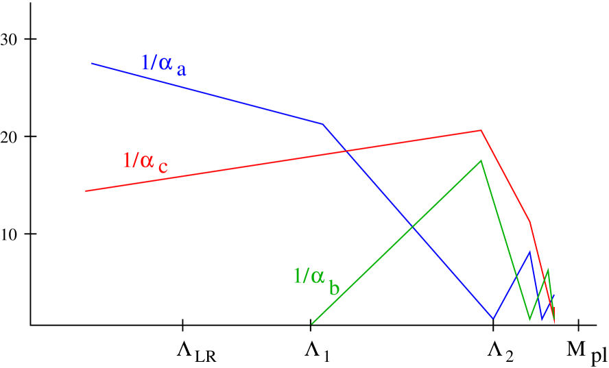
Figure 15: A schematic plot of the running couplings of the three non-abelian gauge groups from $\Lambda_{LR}$ to $M_{Pl}$. In the numeric example, $\Lambda_{LR}\sim 10^{10}$ TeV. The first two Seiberg dualities occur at scale $\Lambda_{1}\sim 10^{11}$ TeV and $\Lambda_{2}\sim 10^{14}$ TeV. The plot shows the acceleration of duality steps and subsequent emergence of a duality wall close to the Planck scale.

Besides the three non-abelian couplings, the LR cascade also has a gauge coupling associated with the $U(1)_{B-L}$ gauge symmetry generated by

$$\mathcal{Q}_{B-L}={\frac{1}{2}}(\mathcal{Q}_{U(1)_{c}}-\mathcal{Q}_{U(1)_{b}}).$$ (59)

This $U(1)_{B-L}$ factor does not actively participate in the Seiberg dualities, and (in our conventions) its beta function is always negative: $\beta=b_{0}/2\pi$ with $b_{0}=-\sum_{\mathrm{i}}q_{i}^{2}$. Given that higher up in the cascade, a large amount of extra matter fields charged under $U(1)_{B-L}$ enter the spectrum, one might be worried that the corresponding coupling may run into a Landau pole at some sub-Planckian scale. However, for the overall $U(1)$ factor inside $U(N)$, fields in the fundamental representation of $SU(N)$ carry $U(1)$ charge $1/N$. This normalization consistently identifies the $U(1)$ symmetry across Seiberg dualities because $SU(N)$ baryons will always have $U(1)$ charge $\pm 1$. Hence, in passing through the subsequent cascade steps, the $U(1)_{B-L}$ charges, and therefore its coupling scale inversely with the rank of the gauge groups. Thus the cascade naturally avoids the Landau pole.

A disadvantage of the cascade scenario is that it does not predict gauge coupling unification. Given that the couplings fluctuate wildly near the UV end of the cascade, any coincidence in the structure of IR couplings would seem accidental. Even so, it is not unnatural that the two non-abelian couplings $\alpha_{c}$ and $\alpha_{a}$ appear to intersect at a scale that is close to the duality wall. Indeed, both couplings are driven to weak coupling at the next-to last stage of the cascade. Gauge coupling unification is the additional coincidence that the hypercharge coupling meets at the same point. This extra coincidence can perhaps be made natural in slightly less minimal versions of the LR cascade which connect to the Standard Model via an intermediate Pati-Salam-like theory, with $U(1)_{B-L}$ and $SU(3)_{c}$ unified into $SU(4)_{c}$. An interesting discussion of gauge coupling unification in D-brane scenarios can be found in [52].

9.2 Energy Scales of the Confining Scenario Cascade

The analysis of the previous section demonstrates that there are a range of energy scales at which node $b$ can first dualize in proceeding from the IR to the UV.  Indeed, once node $b$ deconfines, the resulting gauge group introduces a large number of additional flavors which strongly alter the running of the two $USp$ factors at nodes $a$ and $d$.  Recall that in the case of the confining scenario the gauge coupling at node $a$ approached a Landau pole below the Planck scale only after additional vector-like pairs appeared in the low energy spectrum.  Turning the discussion around, if extra vector-like matter appears at suitably low energy scales, say 1 TeV (perhaps even as a candidate for dark matter) the resulting gauge coupling at node $a$ will suffer from a Landau pole at a sub-Planckian value.  In this case, it is especially natural to Seiberg dualize the theory at energy scales close to this Landau pole. In this section we will assume that this is the scale at which new physics will appear. Depending on the number of vector-like pairs which appear, the duality wall can be at low or high energy scales. For concreteness we keep the duality wall near the Planck scale in the discussion below.

A priori, lowering the Landau pole of node $a$ would still allow a range of values over which node $d$ and then node $a$ could dualize in proceeding from the IR to the UV.  Note, however, that once node $d$ deconfines a large amount of additional tensor matter will now alter the running of the gauge coupling at node $c$.  This will generically cause the coupling constant for node $c$ to approach a Landau pole quite rapidly.  Proceeding from the IR to the UV, the appearance of this Landau pole is in principle problematic because the Landau pole for the gauge coupling at node $a$ may in general lie above that of node $c$.

Recall, however, that a gauge coupling which develops a Landau pole prematurely when additional tensor matter appears cannot arise as part of a consistent RG flow.  In proceeding from the UV to the IR, nodes with a sufficient amount of tensor matter do not dualize during the cascade.  Nevertheless, the resulting value of the gauge coupling may in general be too small to match to observed values.

We now show that the scales of dualization for nodes $a$ and $d$ must indeed be relatively close together so that the Landau pole for the gauge coupling at node $c$ is at a higher scale.  As in the previous section, we shall approximate the running of the couplings by their one loop values.  To keep our discussion as general as possible, we shall at first allow the cascade to ignite via $m$ even vector-like pairs between nodes $d$ and $c$ and nodes $c$ and $a$ and $v$ vector like pairs between nodes $d$ and $E$ and nodes $E$ and $a$, where $E$ denotes a possible extra $U(1)$ flavor node.  For simplicity, we shall assume that the mass of these additional vector-like pairs all enter the low energy spectrum at a scale $\mu=\mu_{new}$.  At scales $\mu_{new}<\mu<\Lambda_{d}$, the running of the couplings for the non-abelian gauge group factors is therefore:

$${2\pi\alpha}_{c}^{-1}\left(\mu\right) =\left(3-2m\right)\log\frac{\mu}{\mu_{new}}+3\log\frac{\mu_{new}}{M}+{2\pi\alpha}_{c}^{-1}\left(M\right)$$ (60)

$${2\pi\alpha}_{a}^{-1}\left(\mu\right) =\left(-1-3m-v\right)\log\frac{\mu}{\mu_{new}}-\log\frac{\mu_{new}}{M}+{2\pi\alpha}_{a}^{-1}\left(M\right)$$ (61)

where to first approximation we may identify $M$ with the mass of the Z boson (91 GeV) and the corresponding couplings as ${2\pi\alpha}_{c}^{-1}\left(M\right)\sim 53$ and ${2\pi\alpha}_{a}^{-1}\left(M\right)\sim 181$.  The approximate energy scale at which ${\alpha}_{a}$ diverges is therefore:

$$\Lambda_{a}=\mu_{new}\left(\frac{\mu_{new}}{M}\right)^{-1/(1+3m+v)}\exp\left(\frac{{2\pi\alpha}_{a}^{-1}\left(M\right)}{1+3m+v}\right)\text{.}$$ (62)

When $\mu_{new}\sim 1$ TeV, the corresponding Landau pole for various values of $m$ and $v$ are:

$$\Lambda_{a}(m =0,v=5)\sim 10^{16}\text{ GeV}$$ (63)

$$\Lambda_{a}(m =2,v=0)\sim 10^{14}\text{ GeV}$$ (64)

so that with only a small amount of additional vector-like matter, the Landau pole for the $a$ node gauge coupling will be significantly smaller.

Once node $d$ deconfines, a large amount of additional matter will accelerate the running of the gauge coupling at node $c$ but at one loop order will not alter that of the gauge coupling at node $a$.  There are two sources of matter which accelerate the running of the $c$ node gauge coupling.  The first is from meson fields which contain bifundamentals between nodes $d$ and $c$.  The tensor matter content once node $d$ deconfines is now $g(1+g+2m)/2$ fields in the $\overline{A}$ and $g(-1+g+2m)/2$ in the $\overline{S}$ of $U(3)$.  In addition, there are $g(g+m)$ fields in the $(\overline{3},\overline{1})$ and $mg$ in the $(3,\overline{1})$ of $U(3)_{c}\times U(1)_{b}$.  The second source of matter corresponds to meson fields which contain bifundamentals between nodes $d$ and $E$.  In this case, there are $gv$ fields in the $(\overline{3},1)$ as well as in the $(\overline{3},\overline{1})$ of $U(3)_{c}\times U(1)_{E}$.  Assuming node $a$ has not dualized, the running of ${\alpha}_{c}^{-1}$ accelerates:

$${2\pi\alpha}_{c}^{-1}\left(\mu\right)=b^{\prime}_{c}\log\frac{\mu}{\Lambda_{d}}+(3-2m)\log\frac{\Lambda_{d}}{\mu_{new}}+3\log\frac{\mu_{new}}{M}+{2\pi\alpha}_{c}^{-1}\left(M\right)$$ (65)

where $b^{\prime}_{c}=-24-31m-6m^{2}-6v-2mv$ when $g=3$.  The corresponding Landau pole is:

$${\Lambda}_{c}=\Lambda_{d}\left(\frac{\Lambda_{d}}{\mu_{new}}\right)^{-(3-2m)/b^{\prime}_{c}}\left(\frac{\mu_{new}}{M}\right)^{-3/b^{\prime}_{c}}\exp\left(\frac{{-2\pi\alpha}_{c}^{-1}\left(M\right)}{b^{\prime}_{c}}\right)\text{.}$$ (66)

Comparing equations (62) and (66), it follows that the denominators of the fractional exponents are significantly larger in the contribution to ${\Lambda}_{c}$ so that ${\Lambda}_{c}$ and $\Lambda_{d}$ will differ by at most only a few orders of magnitude.  In order to match to the observed values of ${\alpha}_{a}^{-1}\left(M\right)$ and ${\alpha}_{c}^{-1}\left(M\right)$, the tensor matter created by dualizing node $d$ must quickly pair up with additional matter created by dualizing node $a$ so that $\Lambda_{a}=\Lambda_{d}$, just as in the left-right symmetric cascade.  Indeed, in retrospect it is immediate that the more general Higgsing scenario cascade will suffer from a similar problem unless nodes $a$ and $d$ dualize at similar energy scales.

When nodes $a$ and $d$ dualize at nearly the same scale, the running of ${\alpha}_{c}^{-1}\left(\mu\right)$ changes to:

$${2\pi\alpha}_{c}^{-1}\left(\mu\right)=b_{c}\log\frac{\mu}{\Lambda_{d}}+(3-2m)\log\frac{\Lambda_{d}}{\mu_{new}}+3\log\frac{\mu_{new}}{M}+{2\pi\alpha}_{c}^{-1}\left(M\right)$$ (67)

where $b_{c}=-15-34m-12m^{2}-6v-4mv$ so that the Landau pole for $\Lambda_{c}$ is:

$$\Lambda_{c}=\Lambda_{d}\left(\frac{\Lambda_{d}}{\mu_{new}}\right)^{-(3-2m)/b_{c}}\left(\frac{\mu_{new}}{M}\right)^{-3/b_{c}}\exp\left(\frac{{-2\pi\alpha}_{c}^{-1}\left(M\right)}{b_{c}}\right)\text{.}$$ (68)

While there is some freedom in choosing the energy scale $\Lambda_{b}$ at which node $b$ deconfines, as in the case of the Higgsing scenario, each subsequent stage of dualization converges rapidly to an accumulation point in the ultraviolet.

9.3 The Duality Wall

The appearance of a duality wall may at first appear to undermine our rationale for selecting a periodic cascade as a candidate UV extension of the MSSM. The wall indeed prevents the cascade from going through a large number of well-separated duality cycles because each successive duality takes place in such a short range of scales that the gauge theory gets trapped in a regime of strong coupling. We interpret this to mean that a purely field theoretic interpretation of Seiberg duality becomes ambiguous. Besides the absence of a weakly coupled limit, the gauge couplings of the system also do not vary slowly enough to give a meaningful definition of the infrared degrees of freedom. In a sense, this is a symptom of the fact that the Planck scale is of finite size. Indeed, in the limit in which the Planck scale decouples, by suitably tuning the couplings of the field theory the accumulation point corresponding to the duality wall can be taken to be arbitrarily large. For this reason it is important to establish that the cascades in question do indeed exhibit a periodic cascading structure which can in principle continue indefinitely. On the other hand, in realistic applications, the finite size of the Planck scale places an upper bound on the value of the energy scale at the duality wall so that the cascade will in practice rapidly become trapped in a regime of strong coupling.

However, in spite of this complication, the appearance of an accelerated cascade with a duality wall in fact helps us, in the following sense. A logarithmic cascade (like the Klebanov Strassler system), while better controlled, would in fact unfold itself too slowly and fail to produce a large $N$ theory at sub-Planckian energy. Precisely because the ranks grow quickly in the accelerated cascade so that the system becomes trapped in a regime of strong coupling, it is natural to expect a dual description of the ultraviolet behavior of the cascading gauge theory in terms of a dual closed string theory on a suitable warped background geometry. Fundamentally, the closed string worldsheets arise via the planar diagrams of the large $N$ theory. When the ’t Hooft coupling is large, the direct geometric description in terms of string theory on a classical background should become better controlled at higher energy scales in the cascade. Although somewhat different from the perspective we have adopted in this paper, another possibility may be that at large $N$ a theory of tensionless strings decoupled from gravity, such as little string theory (LST) may also emerge. Indeed, circumstantial evidence for the appearance of a duality wall in terms of a scale intrinsic to LST has also appeared [38].

10 Candidate D-brane Configurations

We now discuss candidate D-brane configurations which may realize the cascading theories described above.  To this end, we first comment on similarities of the single generation model with the del Pezzo 3 brane probe theory.  As shown in Appendix C, when $g$ is at least three, there is no common conformal window for all the quiver nodes of either the Higgsing or confining scenario.  We next explain what types of restrictions this imposes on any candidate D-brane configuration which realizes the above cascade.

10.1 Single Generation Model and Del Pezzo 3 Probe Theory

Assuming the vector-like Higgs pair has been integrated out by introducing a suitable mass term, when the number of generations $g=1$, reversing all arrows attached to the $D$ node of $Q_{+}$ yields a quiver identical to the del Pezzo 3 brane probe gauge theory.  See figure 16 for a depiction of this theory.  The dimer model for this theory has been treated in [53].  Orientifolds of general dimer models have been treated in [19].  Although we omit the details, a similar cascade to that of the multi-generation model now proceeds provided the gauge group is of type $USp_{a}\times U_{b}\times U_{c}\times SO_{d}$.  Note, however, that whereas any node with tensor matter in the multi-generation model would always flow to weak coupling at low energies, in the single generation model there is far less tensor matter at nodes $b$ and $c$.

Figure 16: A toric phase of the del Pezzo three brane probe theory (b), as well as the orientifold theory when a $SO$ factor is present at node $d$ (a).  The $\mathbb{Z}_{2}$ action of the orientifold leaves fixed the dashed red lines of the dimer model (c).  Deleting the arrows between $B$ and $B^{\prime}$, the connectivity of the quiver theory is identical to that of an octahedron.

10.2 D-Brane Bound States and Non-Conformal Quivers

General arguments from string theory suggest that at low energies, the worldvolume theory of a stack of D3-branes probing a geometric singularity will flow to a non-trivial conformal fixed point.  For more complicated bound states of branes, the resulting low energy theory may not possess such a conformal fixed point.  In either case, the ranks of the quiver gauge theory indicate the brane content of the bound state. Explicit D-brane constructions of semi-realistic Standard Model vacua have been studied in [15]. Our expectation is that a similar brane construction will realize the cascades studied in this paper. The analysis of Appendix C demonstrates that all of the intermediate quiver theories of both the Higgsing and confining scenario cascades do not possess a common conformal window for all quiver nodes.  This presumably indicates that some of the nodes should be thought of as composite objects as was seen in the constructions of [8, 18]. Indeed, it is known that an appropriate Higgsing of the del Pezzo five quiver leads to the MSSM. One might imagine embedding the MSSM in a del Pezzo five cascade, since in this case there is in fact a dual supergravity picture. Moreover, in this case the cascade is approximately conformal, so we can extend the cascade over many more orders of magnitude than the cascades we studied previously, which are limited by the existence of a duality wall.

11 Distinguishing Features of the MSSM

While there are in principle many ways in which a given cascade can terminate, in this section we explain in what sense either cascade scenario distinguishes the MSSM at the bottom of the cascade.  To this end, consider first the Higgsing scenario cascade.  While there is no restriction on the number of Higgs pairs in this case, a non-trivial feature of the Higgsing scenario is that the resulting quiver theory at the bottom of the cascade must contain a $USp(2)$ factor for the weak sector gauge group. From the perspective of the Standard Model, this is a consequence of the fact that once the bifundamental matter content of the Standard Model and in particular the multiplicity of $U$ and $D$ type quarks has been specified, cancellation of non-abelian anomalies for the QCD factor requires a $USp(2N)_{a}\times U(N)_{b}$ gauge group structure. This relation is amplified in the left-right cascade.  Indeed, note that at the final stage of the cascade two of the nodes collapse to a single node.  In the breaking process, bifundamentals charged under the $USp_{d}$ node become the right-handed $U$ and $D$ type quarks.  In the event that the rank of the $d$ node gauge group had been larger, additional bifundamental matter would exist in the Higgsed quiver theory.  This in turn implies that the gauge group factor of the extra $d$ node must be $USp(2)$.  Prior to Higgsing, the non-abelian anomalies at node $c$ vanish only when the gauge group factor at node $a$ is $USp(2)$.

In the context of the confining scenario, the multiplicity of $U$ and $D$ type quarks relates to the rank of the $USp_{a}$ factor for a different reason.  Consider a more general class of quiver theories such that nodes $a$ and $d$ attach to additional vector-like pairs.  Indeed, in order to properly accelerate the cascade we must allow such vector-like pairs.  To maintain the repeating structure of the cascade, these additional pairs must attach in a symmetric fashion to both nodes $a$ and $d$.  Recall that at the bottom of the cascade in the confining scenario, both nodes $d$ and $b$ confine without breaking chiral symmetry.  Before nodes $a$ and $d$ dualize for the last time to reach the quiver theory $q_{+}$,  the corresponding quiver theory will be given by $adq_{+}$ and will not contain any tensor matter.  Even if node $b$ has already confined, in order to cancel the potential non-abelian anomaly present at node $c$, the ranks of the $USp$ factors at nodes $a$ and $d$ must be identical.  As argued previously, node $d$ must confine without breaking chiral symmetry.  Prior to confinement, it follows that when the gauge group factor is $USp(2N_{d})$, precisely $F_{d}=2N_{d}+4$ bifundamentals (counted with appropriate multiplicity) attach to node $d$.  Besides the single Higgs pair, each vector-like pair attached to node $a$ has a symmetric counterpart attached to node $d$.  It therefore follows that $F_{a}=2N_{d}+4+2N_{b}$ bifundamentals attach to node $a$.  Dualizing node $a$ now yields the gauge group factor $USp(2N_{b})$ when a single Higgs pair is present.  Because the $U$ and $D$ type quarks arise as dual meson fields, the number of Higgs pairs also determines their multiplicity. In this way the multiplicity of quarks and the $USp(2)$ gauge group factor both get related to the fact that there is a single Higgs pair.  Viewed in this light, it is interesting to note that the beta function of the $SU(2)$ gauge coupling switches sign in going from the Standard Model to the MSSM.

Turning the discussion around, note that the gauge group of the MQSM can only be reached in the confining scenario when there is a single Higgs pair.  Indeed, while required in order for intermediate stages of the cascade to proceed, the presence of this pair is also necessary to achieve the correct gauge group assignment at the bottom of the cascade.  The precise Higgs regeneration mechanism discussed previously also requires a particular set of conditions to be met by the topology of the MQSM.  For example, RG node locking will occur provided $g\geq 3$.  In the more general scenario where an additional $m$ vector-like pairs attach between node $c$ and $a$, the analysis of section 6.6 demonstrates that the Higgs regeneration mechanism will proceed only when $m$ is an even number and $g$ is an odd number. In other words, the number of generations must be odd in order for the cascade to proceed. It would be interesting to establish whether further restrictions require $g$ to be exactly three.

12 Discussion

If the Standard Model or some supersymmetric extension thereof is realized on a stack of D-branes, general considerations from string theory greatly restrict possible ways in which extra matter can enter the low energy spectrum.  In the context of D-brane constructions probing local geometries, it is also natural to treat the large $N$ limit of such configurations. When the ranks of the gauge groups change so as to perturb the system away from a conformal fixed point, such theories will undergo RG flow and will typically undergo a duality cascade.  In this paper we have considered an explicit minimal realization of this paradigm where the connectivity of the cascading quiver must periodically repeat to its original form such that the MSSM appears at the very bottom of the duality cascade.  We have presented two generic ways in which a four node quiver can cascade to the MSSM depending on whether at the final stages the extra node Higgses or confines.  In both cases, we have found a rather rigid structure which in fact unifies in the ultraviolet.  Indeed, at higher energies the only difference between the Higgsing scenario and the confining scenario corresponds to the presence of an additional vector-like pair.  Higgsing to the MQSM represents the most minimal cascading quiver which can descend to the MQSM.  It is intriguing that the left-right symmetric extension of the MSSM naturally comes equipped with a cascading structure.  In the context of the confining scenario we have found an intricate sequence of dualities which in fact require a single Higgs pair in order for the cascade to proceed.  Moreover, we have also presented a general mechanism whereby this Higgs pair can appear and disappear as the cascade proceeds to lower energies.  This has the appealing feature that the minimal confining cascade scenario implies a naturally light Higgs pair.

Much of the above discussion must of course be tempered by phenomenological considerations.  While the phenomenology of the Higgsing scenario has been studied in the context of left-right symmetric extensions of the Standard Model, it would be interesting to determine the precise distinction between such partial unification schemes and cascading scenarios.  By comparison with the Higgsing scenario, the matter content and running of the couplings is far less flexible in the confining scenario.  Due to the intriguing prediction of a single Higgs pair, it would be interesting to see whether further phenomenological considerations apply.  As some possibilities, we now discuss both right-handed neutrinos and CKM matrix elements in the MSSM.

Whereas right-handed neutrinos naturally appear at the last stage of the Higgsing scenario as matter transforming in the adjoint of node $b$, in the confining scenario these fields can appear as dual mesons charged under the adjoint of node $b$.  This would suggest that in either scenario, one natural possibility is to have the Majorana mass of the right-handed neutrinos near energy scales set by the bottom of the cascade.

It is also of interest to determine whether the cascading scenario naturally imposes any restrictions on the Yukawa couplings of the MSSM.  Such constraints translate into restrictions on the mixing between generations of the right-handed quarks known as the CKM matrix.  While this is essentially a generic parameter in the context of the Higgsing scenario, for the confining scenario, the explicit method of Higgs regeneration discussed in section 6.5 required that all terms of the superpotential remain invariant under a general $\mathbb{Z}_{2}$ reflection symmetry of the oriented covering theory.  In the orientifold theory, this descends to the condition that the up and down type Yukawa couplings are in fact identical.  At zeroth order, this would imply that the CKM matrix is diagonal.  Note that no similar relation exists for the mixing of neutrinos. This structure for the mixings is, to leading order what one would expect based on the observed values of the CKM and MNS mixing matrices.

Perhaps the most outstanding issue in this context is how supersymmetry is broken near the bottom of the cascade.  While we have proposed some general possibilities where supersymmetry breaking communicates via the extra node, these scenarios appear to produce a splitting between the W bosons and winos which is too small.  It would be interesting to see whether other minimal cascading scenarios can naturally accomodate supersymmetry breaking.

Proceeding from the IR to the UV, we have found that the ranks of the gauge group factors participating in the cascade rapidly increase.  This leads to a large increase in the number of field degrees of freedom in the corresponding gauge theory.  It is tempting to speculate that this increase in the number of degrees of freedom has some relation to other phenomena in string theory where a large profusion of states appear at a critical temperature, such as in the Hagedorn phase transition.

The appearance of the duality wall appears unavoidable and may lead to potentially interesting consequences for cosmology. We now briefly speculate on some possibilities. At higher and higher temperatures an increasing number of matter fields appear. In a dual gravity description at least one extra spatial dimension will appear to decompactify at higher energy scales. Said differently, as the universe cools, such a cosmology will compactify the extra dimensions. Roughly speaking the compactification process would likely begin at high scales where the wall starts to appear. Near the energy scale where the final dualization occurs, the resulting theory would then be best described as an an effective four dimensional theory. In view of the concrete gauge theory realization of this growth in the number of degrees of freedom at higher energy scales, it would be interesting to study such issues in further detail.

Appendices

Appendix A Partial Classification of Cascading Quivers

In this Appendix we partially classify candidate cascade paths for single node extensions of the covering theory of the MQSM by purely chiral matter which can descend to a cascade in the orientifold theory.  To keep our discussion as general as possible we shall allow $n$ Higgs pairs but otherwise no additional vector-like matter.  Assigning gauge group ranks compatible with the $\mathbb{Z}_{2}$ orientifold symmetry, we find that cancelling all non-abelian anomalies greatly restricts the ways in which the extra node can attach to the MQSM.  Restricting to this class of quiver topologies, we next consider candidate cascades.  We find that unless the arrows of the covering theory have multiplicity $g$, a cascade in the covering theory will not properly descend to the orientifold theory.

When the number of generations $g$ is greater than one there is a unique way to attach one additional node by purely chiral matter to the covering quiver of the MQSM so that the resulting quiver admits a cascade which repeats after finitely many steps.  Let the signed integers $n_{DA}$, $n_{DB}$, $n_{DB^{\prime}}$, $n_{DC}$, $n_{DC^{\prime}}$ denote the number of bifundamentals in the covering theory charged in the fundamental representation of node $D$, where a negative number indicates that the orientation of the arrow is reversed.  The $\mathbb{Z}_{2}$ symmetry of the quiver imposes the constraint:

$$n_{DB}=-n_{DB^{\prime}}\qquad\qquad n_{DC}=-n_{DC^{\prime}}\text{.}$$ (69)

Due to the fact that the cascade must repeat, we may assume that the ranks of all gauge groups factors are greater than one.  The non-abelian anomalies of the covering theory gauge groups vanish when:

$$n_{DA} =0$$

$$n_{DC}N_{D}-2gN_{B}+gN_{A} =0$$ (70)

$$n_{DB}N_{D}-2gN_{B}+gN_{A} =0$$

where in the above we have used the fact that the $\mathbb{Z}_{2}$ symmetry of the quiver imposes the constraints $N_{B}=N_{B^{\prime}}$ and $N_{C}=N_{C^{\prime}}$.  This implies:

$$n_{DB}=n_{DC}\text{.}$$ (71)

We therefore conclude that for a given positive integer $\alpha=\left|n_{DB}\right|$, there are two candidate single node extensions of the covering quiver theory which we denote by $Q_{+}$ and $Q_{-}$ for $n_{DB}$ respectively positive or negative (see figure 8).

We now argue that when $g>1$, the quiver theory $Q_{-}$ does not admit a sequence of Seiberg dualities leading to a repeating cascade structure.  To this end, we show that each candidate cascade only proceeds a finite number of steps.  Because too much bifundamental matter connects $B$ to $B^{\prime}$, the only admissible Seiberg dual quiver theories are $AQ_{-}$, $DQ_{-}$ and $CC^{\prime}Q_{-}$.  First consider the quiver theories $AQ_{-}$ and $DQ_{-}$.  Because no bifundamentals connect $A$ to $D$ and because there exist bifundamentals connecting the pair $BB^{\prime}$ as well as the pair $CC^{\prime}$, the next stage of the cascade is $ADQ_{-}$.  Due to the presence of massless vector-like matter connecting $A$ to $B$ as well as $A$ to $B^{\prime}$, dualizing node $A$ yields $(g+n)^{2}$ meson fields connecting $B$ to $B^{\prime}$ and $n^{2}$ meson fields connecting $B^{\prime}$ to $B$.  Integrating out all vector-like pairs other than those between $A$ and $B$ and $A$ and $B^{\prime}$, the net number of bifundamentals from $C$ to $C^{\prime}$ and the number from $B$ to $B^{\prime}$ is:

$$n_{CC^{\prime}} =g^{2}+\alpha^{2}>0$$

$$n_{BB^{\prime}} =g^{2}+\alpha^{2}+2g(n-1)>0\text{.}$$ (72)

We therefore conclude that for $g>1$ a $\mathbb{Z}_{2}$ symmetric cascade cannot proceed.

Next consider the quiver theory $CC^{\prime}Q_{-}$.  The next stage of dualization now leads uniquely to the quiver theory $ADCC^{\prime}Q_{-}$.  As in the previous case, the cascade cannot proceed because the number of bifundamentals from $C^{\prime}$ to $C$ and the number from $B$ to $B^{\prime}$ is:

$$n_{C^{\prime}C} =g^{2}+\alpha^{2}>0$$

$$n_{BB^{\prime}} =g^{2}+\alpha^{2}+2g(n-1)>0\text{.}$$ (73)

Hence, the quiver theory $Q_{-}$ does not admit a periodically repeating cascade.

We now show that the remaining candidate quiver theory $Q_{+}$ only admits a repeating cascade which descends to the orientifold theory when $\alpha=g$.  To begin, first consider a cascade which dualizes node $A$ or $D$ of the quiver theory $Q_{+}$.  This produces a quiver theory with bifundamentals between the pair $B$ and $B^{\prime}$ and the pair $C$ and $C^{\prime}$ so that the next stage of dualization always leads to the quiver theory $ADQ_{+}$.  Due to the different direction of orientation for all arrows attached to node $D$, the number of bifundamentals from $C^{\prime}$ to $C$ and the number from $B$ to $B^{\prime}$ is:

$$n_{C^{\prime}C} =\alpha^{2}-g^{2}$$ (74)

$$n_{BB^{\prime}} =g^{2}-\alpha^{2}+2g(n-1)\text{.}$$

It follows that the cascade can only proceed provided $\alpha=mg$ for some positive integer $m$ so that:

$$n_{C^{\prime}C} =g^{2}(m^{2}-1)$$ (75)

$$n_{BB^{\prime}} =g^{2}(1-m^{2})+2g(n-1)\text{.}$$

When $m>1$, the resulting cascade cannot proceed unless $n_{BB^{\prime}}$ vanishes.  In this case:

$$n=\frac{g\left(m^{2}-1\right)}{2}+1>1\text{.}$$ (76)

To proceed further, it is most efficient to descend to the orientifold theory and ask whether the above assignment of Higgs pairs eliminates all tensor matter.  A priori, the additional node $D$ can descend to either a $SO$ or $USp$ type factor.  It follows from the general analysis of Seiberg duality for $USp$ and $SO$ type factors given in section 3.1 that dualizing the pair of nodes $a$ and $d$ in the orientifold theory $q_{+}$ generates additional tensor matter at node $b$.  Letting $\varepsilon=+1$ (resp. $-1$) when node $d$ corresponds to an $SO$ (resp. $USp$) type factor, the total amount of tensor matter at node $b$ is:

Node b $$\text{: }g\overline{S_{b}}+g\overline{A_{b}}+\frac{\alpha(\alpha+\varepsilon)}{2}\overline{S_{b}}+\frac{\alpha(\alpha-\varepsilon)}{2}\overline{A_{b}}+\frac{n(n+1)}{2}\overline{A_{b}}+\frac{n(n-1)}{2}\overline{S_{b}}$$ (77)

$$+\frac{\left(g+n+1\right)(g+n)}{2}S_{b}+\frac{\left(g+n-1\right)(g+n)}{2}A_{b}$$ (78)

$$=\text{ \ }\frac{1}{2}\left(g^{2}+g(2n-3)-\alpha\left(\alpha+\varepsilon\right)\right)S_{b}$$ (79)

$$+\frac{1}{2}\left(g^{2}+g(2n-1)+\alpha\left(-\alpha+\varepsilon\right)\right)A_{b}$$ (80)

where in the above, lines (77) and (78) denote all tensor matter created by dualizing nodes $a$ and $d$ and lines (79) and (80) denote the total amount after all vector-like pairs have been integrated out. If all vector-like pairs do indeed cancel so that node $b$ is free to dualize, the two coefficients multiplying $S_{b}$ and $A_{b}$ in lines (79) and (80) respectively must separately vanish.  We note in passing that because the multiplicity of each type of tensor matter is divisible by $g$, the corresponding node will indeed “RG lock” if the amount of uncancelled tensor matter is non-zero.  Subtracting the two coefficients yields the condition:

$$-g-\alpha\varepsilon=0\text{.}$$ (81)

Because $\alpha$ is a positive integer, the above equality will hold only when $\alpha=g$ and $\varepsilon=-1$ so that the gauge group factor at node $d$ is of $USp$ type.

To complete our analysis, we now establish that the existence of a repeating cascade structure for the quiver $CC^{\prime}Q_{+}$ which properly descends to the orientifold also requires $\alpha=g$.  The essential point is that after cancelling all vector-like pairs, dualizing the pair $CC^{\prime}$ only re-orients arrows attached to this pair of nodes and otherwise leaves the quiver theory unchanged.  As in the quiver theory $ADQ_{+}$ and its orientifold descendant, the tensor matter of the theory $adcq_{+}$ can only cancel when equation (81) holds.

Appendix B Dual Superpotentials

As argued in section 6.4, because each stage of the confining cascade scenario must eventually pass through the quiver theory $adq_{+}$, $q_{+}$ or a similar quiver theory with the orientations of some arrows reversed, it is enough to analyze only these theories and their immediate Seiberg duals.  In this Appendix we collect the explicit expressions for the superpotential of all possible duals of the quiver theories $adq_{+}$ and $q_{+}$.  We perform this analysis to explicitly demonstrate that generic cubic and quartic terms of the electric theory will indeed lift nearly all vector-like pairs in the dual magnetic theory.  In the absence of restrictions on the form of the couplings, this analysis corresponds to classifying all possible paths in the quiver theory with a given number of link fields.  In the presence of symmetries of the string theory or field theory, there will be further restrictions on the form of the couplings.  For this reason, it is also important to establish that a given symmetry does not forbid (resp. does forbid) a given vector-like pair from developing a mass.  Indeed, in the minimal realization of the cascading scenario which terminates via confinement, we must establish that the massless Higgs pair does not develop a $\mu$ term at some further stage of the cascade. While we shall present this analysis for quiver theories where the superpotential is generically not invariant under matter parity, by suitably restricting the form of the coupling constant matrices, a similar discussion holds in this case as well.

We now classify all terms of the superpotential of degree four or less in the quiver theory $adq_{+}$.  By inspection, this quiver is identical to figure 10$d)$.  Further, the absence of closed triangles in the theory implies that all gauge invariant operators are of even degree in the quiver fields.  Labeling the various chiral superfields by the variable $X$, we shall distinguish which gauge group a given field is charged under as well as whether it is a fundamental or anti-fundamental index by the subscript of the field. To avoid cluttering the notation too much, we shall suppress the presence of the appropriate $\epsilon$ tensors necessary for contracting all $USp$ indices.  While this notation admittedly obscures the connection of the $X$ fields to the content of the MQSM, it will prove convenient in discussing the magnetic dual superpotentials.  The superpotential for the quiver theory $adq_{+}$ is:

$$W_{adq_{+}} =\mu_{I}X_{ab}X_{\overline{b}a}^{I}+\alpha_{ijkl}X_{dc}^{i}X_{\overline{c}a}^{j}X_{a\overline{c^{\prime}}}^{k}X_{c^{\prime}d}^{l}$$

$$+\beta_{ijk}^{I}X_{dc}^{i}X_{\overline{c}a}^{j}X_{a\overline{b}}^{I}X_{bd}^{k}+\gamma_{ij}^{IJ}X_{db}^{i}X_{\overline{b}a}^{I}X_{a\overline{b^{\prime}}}^{J}X_{b^{\prime}d}^{j}$$

$$+\mu_{IJ}\left(X_{ab}X_{\overline{b}a}^{I}\right)\left(X_{a^{\prime}b^{\prime}}X_{\overline{b^{\prime}}a^{\prime}}^{J}\right)$$ (82)

$$+\kappa_{IJ}X_{ab}X_{\overline{b}a^{\prime}}^{I}X_{a^{\prime}b^{\prime}}X_{\overline{b^{\prime}}a}^{J}+\widehat{\kappa}_{IJ}X_{ab}X_{\overline{b}a^{\prime}}^{I}X_{a^{\prime}\overline{b^{\prime}}}^{J}X_{b^{\prime}a}+\widehat{\mathcal{O}}_{6}$$

where in the above, the indices $i,j,k,l$ run from $1,...,g$, $I$ and $J$ run from $I=0,1,...,g$ and $\widehat{\mathcal{O}}_{6}$ denotes all degree six and higher gauge invariant combinations of fields.

Dualizing the pair of nodes $a$ and $d$ in $adq_{+}$ produces the magnetic dual superpotential:

$$W_{ad(adq_{+})} =W_{adq_{+}}|_{M={\mu}^{-1}XY}+W_{meson}=\mu_{a}\mu_{I}A_{\overline{b}b}^{I}$$

$$+\mu_{a}\mu_{d}\alpha_{ijkl}\left(A_{[\overline{cc^{\prime}}]}^{(jk)}+A_{(\overline{cc^{\prime}})}^{[jk]}\right)\left(D_{[cc^{\prime}]}^{(jk)}+D_{(cc^{\prime})}^{[jk]}\right)$$

$$+\mu_{a}\mu_{d}\beta_{ijk}^{I}A_{\overline{cb}}^{jI}D_{bc}^{ik}+\mu_{a}\mu_{d}\gamma_{ij}^{IJ}\left(A_{[\overline{bb^{\prime}}]}^{(IJ)}+A_{(\overline{bb^{\prime}})}^{[IJ]}\right)\left(D_{[bb^{\prime}]}^{(jk)}+D_{(bb^{\prime})}^{[jk]}\right)$$

$$+\mu_{a}^{2}\mu_{IJ}\left(A_{\overline{b}b}^{I}\right)\left(A_{\overline{b^{\prime}}b^{\prime}}^{J}\right)+\mu_{a}^{2}\kappa_{IJ}A_{\overline{b}b^{\prime}}^{I}A_{\overline{b^{\prime}}b}^{J}+\mu_{a}^{2}\widehat{\kappa}_{IJ}A_{[\overline{bb^{\prime}}]}^{(IJ)}A_{[b^{\prime}b]}$$ (83)

$$+\left(D_{[cc^{\prime}]}^{(ij)}+D_{(cc^{\prime})}^{[ij]}\right)X_{\overline{c^{\prime}}d}^{j}X_{d\overline{c}}^{i}+\left(D_{[bb^{\prime}]}^{(ij)}+D_{(bb^{\prime})}^{[ij]}\right)X_{\overline{b^{\prime}}d}^{j}X_{d\overline{b}}^{i}+D_{bc}^{ij}X_{\overline{c}d}^{j}X_{d\overline{b}}^{i}$$

$$+\left(A_{[\overline{cc^{\prime}}]}^{(jk)}+A_{(\overline{cc^{\prime}})}^{[jk]}\right)X_{c^{\prime}a}^{j}X_{ac}^{i}+\left(A_{[\overline{bb^{\prime}}]}^{(IJ)}+A_{(\overline{bb^{\prime}})}^{[IJ]}\right)X_{b^{\prime}a}^{J}X_{ab}^{I}$$

$$+A_{[bb^{\prime}]}X_{\overline{b^{\prime}}d}X_{d\overline{b}}+A_{b\overline{b^{\prime}}}^{I}X_{b^{\prime}a}^{I}X_{a\overline{b}}+A_{b\overline{c}}^{i}X_{ca}^{i}X_{a\overline{b}}+A_{\overline{bc}}^{iI}X_{ca}^{i}X_{ab}^{I}+\widehat{\mathcal{O}}_{4}\text{.}$$

In the above, the fields $A$ and $D$ denote dual meson fields generated by dualizing the nodes $a$ and $d$, respectively.  The symmetrization and anti-symmetrization of a pair of indices indicates the number of such meson fields.  Assuming that the term $\mu_{I}$ has been set to zero, we note that for generic values of the couplings, no linear terms are present in the superpotential.  By inspection of the degree two terms of $W_{ad(adq_{+})}$, we note that all of the $A$ tensor matter at node $c$ pairs with $D$ tensor matter at node $c$ via the $\alpha$ couplings.  On the other hand, the quadratic term for the $A$ tensor matter at node $b$ is schematically of the form:

$$W_{ad(adq_{+})} \supset\left[D^{(ij)},A\right]_{1\times g(g+1)/2+1}\left[M^{symm}\right]_{g(g+1)/2+1\times(g+1)(g+2)/2}\left[A^{(IJ)}\right]_{(g+1)(g+2)/2\times 1}$$

$$+\left[D^{[ij]}\right]_{1\times g(g-1)/2}\left[M^{asymm}\right]_{g(g-1)/2\times(g+1)g/2}\left[A^{[IJ]}\right]_{(g+1)g/2\times 1}$$

where the $M$’s denote a generic matrix and the subscripts for each square bracket indicates the size of the corresponding matrix.  We therefore conclude that for generic couplings, precisely $g$ two index symmetric and anti-symmetric tensor matter fields at node $b$ remain massless.  Further, we note that the remaining $A$ fields in the adjoint representation at node $b$ develop a mass due to the couplings $\mu_{IJ}$ and $\kappa_{IJ}$.  Finally, it follows from the general form of the coupling $\beta$ that only $g^{2}$ of the $A_{\overline{cb}}^{jI}$ develop a mass by pairing with $D$ fields.  This again leaves precisely $g$ massless fields.  Note, however, that when the linear term proportional to $\mu_{I}A_{\overline{b}b}^{I}$ is absent, it is consistent to set the vevs of all fields to zero.  In this case, there are no quadratic terms of the form $X_{a\overline{b}}X_{ab}^{I}$.  In other words, once set to zero, the $\mu$-term for the Higgs pair remains zero.

Dualizing node $b$ produces the magnetic dual superpotential:

$$W_{b(adq_{+})} =\mu_{b}\mu_{I}B_{aa}^{I}+\mu_{b}^{2}\gamma_{ij}^{IJ}B_{da}^{iI}B_{ad}^{Jj}+\mu_{b}^{2}\mu_{IJ}\left(B_{aa}^{I}\right)\left(B_{a^{\prime}a^{\prime}}^{J}\right)$$

$$+\mu_{b}^{2}\kappa_{IJ}B_{aa^{\prime}}^{I}B_{a^{\prime}a}^{J}+\mu_{b}^{2}\widehat{\kappa}_{IJ}B_{aa^{\prime}}^{I}B_{a^{\prime}a}^{J}$$

$$+\mu_{b}\beta_{ijk}^{I}X_{dc}^{i}X_{\overline{c}a}^{j}B_{ad}^{kI}+B_{ad}^{iI}X_{d\overline{b}}^{i}X_{ba}^{I}+B_{aa^{\prime}}^{I}X_{a^{\prime}b}^{I}X_{\overline{b}a}$$ (84)

$$+B_{aa^{\prime}}^{I}X_{a^{\prime}\overline{b}}X_{ba}^{I}+\alpha_{ijkl}X_{dc}^{i}X_{\overline{c}a}^{j}X_{a\overline{c^{\prime}}}^{k}X_{c^{\prime}d}^{l}+\widehat{\mathcal{O}}_{4}\text{.}$$

We note that the meson fields $B$ between nodes $a$ and $d$ all develop a mass due to the $\gamma$ couplings and the $B$ adjoint fields at node $a$ all develop a mass due to $\mu,\kappa$ and $\widehat{\kappa}$.  As before, the dual theory does not contain a generalized $\mu$-term.

A similar analysis establishes that dualizing node $c$ produces the superpotential:

$$W_{c(adq_{+})} =\mu_{I}X_{ab}X_{\overline{b}a}^{I}+\mu_{c}^{2}\alpha_{ijkl}C_{da}^{ij}C_{ad}^{kl}+C_{ad}^{ij}X_{d\overline{c}}^{i}X_{ca}^{j}$$

$$+\mu_{c}\beta_{ijk}^{I}C_{da}^{ij}X_{a\overline{b}}^{I}X_{bd}^{k}+\gamma_{ij}^{IJ}X_{db}^{i}X_{\overline{b}a}^{I}X_{a\overline{b^{\prime}}}^{J}X_{b^{\prime}d}^{j}$$

$$+\mu_{IJ}\left(X_{ab}X_{\overline{b}a}^{I}\right)\left(X_{a^{\prime}b^{\prime}}X_{\overline{b^{\prime}}a^{\prime}}^{J}\right)$$ (85)

$$+\kappa_{IJ}X_{ab}X_{\overline{b}a^{\prime}}^{I}X_{a^{\prime}b^{\prime}}X_{\overline{b^{\prime}}a}^{J}+\widehat{\kappa}_{IJ}X_{ab}X_{\overline{b}a^{\prime}}^{I}X_{a^{\prime}\overline{b^{\prime}}}^{J}X_{b^{\prime}a}+\widehat{\mathcal{O}}_{4}$$

so that all of the meson fields $C$ between nodes $a$ and $d$ develop a mass due to the $\alpha$ couplings.

To summarize, the above analysis establishes that a $\mu$ term will never appear by dualizing a node in the theory $adq_{+}$.  We now show that whereas dualizing the pair $ad$ in $q_{+}$ also does not produce a $\mu$ term, such a term does appear upon dualizing node $c$.

We begin by classifying all terms of the superpotential of degree four or less in the quiver theory $q_{+}$:

$$W_{q_{+}} =\mu_{I}X_{a\overline{b}}X_{ba}^{I}$$

$$+\lambda_{ij}X_{ca}^{i}X_{a\overline{b}}X_{b\overline{c}}^{j}+\widehat{\lambda}_{ij}^{I}X_{ca}^{i}X_{ab}^{I}X_{\overline{bc}}^{j}+\sigma_{i}^{IJ}X_{ab}^{I}X_{(\overline{bb^{\prime}})}^{i}X_{b^{\prime}a}^{J}+\rho_{i}^{IJ}X_{ab}^{I}X_{[\overline{bb^{\prime}}]}^{i}X_{b^{\prime}a}^{J}$$

$$+\alpha_{ijkl}X_{d\overline{c}}^{i}X_{ca}^{j}X_{ac^{\prime}}^{k}X_{\overline{c^{\prime}}d}^{l}+\beta_{ijk}^{I}X_{d\overline{c}}^{i}X_{ca}^{j}X_{ab}^{I}X_{\overline{b}d}^{k}+\gamma_{ij}^{IJ}X_{d\overline{b}}^{i}X_{ba}^{I}X_{ab^{\prime}}^{J}X_{\overline{b^{\prime}}d}^{j}$$

$$+\tau_{ijk}^{I}X_{ac}^{i}X_{\overline{c}b}^{j}X_{(\overline{bb^{\prime}})}^{k}X_{b^{\prime}a}^{I}+\omega_{ijk}^{I}X_{ac}^{i}X_{\overline{c}b}^{j}X_{[\overline{bb^{\prime}}]}^{k}X_{b^{\prime}a}^{I}$$

$$+\varphi_{ijkl}X_{ac}^{i}X_{\overline{cb}}^{j}X_{b\overline{c^{\prime}}}^{k}X_{c^{\prime}a}^{l}$$ (86)

$$+\mu_{IJ}\left(X_{ab}X_{\overline{b}a}^{I}\right)\left(X_{a^{\prime}b^{\prime}}X_{\overline{b^{\prime}}a^{\prime}}^{J}\right)+\kappa_{IJ}X_{ab}X_{\overline{b}a^{\prime}}^{I}X_{a^{\prime}b^{\prime}}X_{\overline{b^{\prime}}a}^{J}$$

$$+\widehat{\kappa}_{IJ}X_{ab}X_{\overline{b}a^{\prime}}^{I}X_{a^{\prime}\overline{b^{\prime}}}^{J}X_{b^{\prime}a}+\widehat{\mathcal{O}}_{5}\text{.}$$

Note in particular that the chiral fields attached to node $d$ first contribute at quartic order.  Due to the fact that node $b$ contains too much tensor matter, any candidate cascade must proceed by dualizing the pair of nodes $ad$ or the node $c$.  Dualizing $ad$ yields the superpotential:

$$W_{ad(q_{+})} =\mu_{a}\mu_{I}A_{b\overline{b}}^{I}+\mu_{a}\lambda_{ij}A_{c\overline{b}}^{i}X_{b\overline{c}}^{j}+\mu_{a}\widehat{\lambda}_{ij}^{I}A_{cb}^{iI}X_{\overline{bc}}^{j}$$

$$+\mu_{a}\sigma_{i}^{IJ}X_{(\overline{bb^{\prime}})}^{i}A_{(b^{\prime}b)}^{[JI]}+\mu_{a}\rho_{i}^{IJ}X_{[\overline{bb^{\prime}}]}^{i}A_{[b^{\prime}b]}^{(JI)}$$

$$+\mu_{a}^{2}\mu_{IJ}\left(A_{b\overline{b}}^{I}\right)\left(A_{b^{\prime}\overline{b^{\prime}}}^{J}\right)+\mu_{a}^{2}\kappa_{IJ}A_{\overline{b}b^{\prime}}^{I}A_{\overline{b^{\prime}}b}^{J}+\mu_{a}^{2}\widehat{\kappa}_{IJ}A_{[\overline{bb^{\prime}}]}^{(IJ)}A_{[b^{\prime}b]}$$

$$+\mu_{a}\mu_{d}\alpha_{ijkl}\left(A_{[cc^{\prime}]}^{(jk)}+A_{(cc^{\prime})}^{[jk]}\right)\left(D_{[\overline{c^{\prime}c}]}^{(jk)}+D_{(\overline{c^{\prime}c})}^{[jk]}\right)+\mu_{a}\mu_{d}\beta_{ijk}^{I}A_{cb}^{jI}D_{\overline{bc}}^{ki}$$

$$+\mu_{a}\mu_{d}\gamma_{ij}^{IJ}\left(A_{[bb^{\prime}]}^{(IJ)}+A_{(bb^{\prime})}^{[IJ]}\right)\left(D_{[\overline{b^{\prime}b}]}^{(ji)}+D_{(\overline{b^{\prime}b})}^{[ji]}\right)$$ (87)

$$+\mu_{a}\tau_{ijk}^{I}X_{\overline{c}b}^{j}X_{(\overline{bb^{\prime}})}^{k}A_{b^{\prime}c}^{Ii}+\mu_{a}\omega_{ijk}^{I}X_{\overline{c}b}^{j}X_{[\overline{bb^{\prime}}]}^{k}A_{b^{\prime}c}^{Ii}$$

$$+\mu_{a}\varphi_{ijkl}X_{\overline{cb}}^{j}X_{b\overline{c^{\prime}}}^{k}\left(A_{[c^{\prime}c]}^{(li)}+A_{(c^{\prime}c)}^{[li]}\right)$$

$$+A_{b\overline{b^{\prime}}}^{I}X_{b^{\prime}a}^{I}X_{a\overline{b}}+\left(D_{[\overline{bb^{\prime}}]}^{(ij)}+D_{(\overline{bb^{\prime}})}^{[ij]}\right)X_{b^{\prime}d}^{i}X_{db}^{j}$$

$$+\left(A_{[bb^{\prime}]}^{(IJ)}+A_{(bb^{\prime})}^{[IJ]}\right)X_{\overline{b^{\prime}}a}^{I}X_{a\overline{b}}^{J}+A_{[\overline{bb^{\prime}}]}X_{b^{\prime}a}X_{ab}$$

$$+\left(D_{[\overline{cc^{\prime}}]}^{(ij)}+D_{(\overline{cc^{\prime}})}^{[ij]}\right)X_{c^{\prime}d}^{i}X_{dc}^{j}+\left(A_{[cc^{\prime}]}^{(ij)}+A_{(cc^{\prime})}^{[ij]}\right)X_{\overline{c^{\prime}}a}^{I}X_{a\overline{c}}^{J}$$

$$+D_{\overline{bc}}^{ij}X_{cd}^{j}X_{db}^{i}+A_{c\overline{b}}^{i}X_{ba}X_{a\overline{c}}^{i}+A_{cb}^{iI}X_{\overline{b}a}^{I}X_{a\overline{c}}^{i}+\widehat{\mathcal{O}}_{3}\text{.}$$

By inspection, when $\mu_{I}$ vanishes, all vector-like pairs other than the Higgs pair develop a mass.  As before, we therefore conclude that once the generalized $\mu$-term has been set to zero, for generic values of the couplings it will not regenerate.

The final way in which the quiver theory $q_{+}$ can dualize is via node $c$.  In fact, it can be shown by analyzing all possible candidate paths that each candidate cascade must eventually dualize node $c$ in either the quiver theory $q_{+}$ or its conjugate with all arrow directions reversed.  Dualizing node $c$ yields the superpotential:

$$W_{c(q_{+})} =\mu_{I}X_{a\overline{b}}X_{ba}^{I}+\mu_{c}\lambda_{ij}X_{a\overline{b}}C_{ba}^{ji}+\mu_{c}\widehat{\lambda}_{ij}^{I}X_{ab}^{I}C_{\overline{b}a}^{ji}$$

$$+\mu_{c}^{2}\varphi_{ijkl}C_{a\overline{b}}^{ij}C_{ba}^{kl}+\mu_{c}^{2}\alpha_{ijkl}C_{da}^{ij}C_{ad}^{kl}$$

$$+\sigma_{i}^{IJ}X_{ab}^{I}X_{(\overline{bb^{\prime}})}^{i}X_{b^{\prime}a}^{J}+\rho_{i}^{IJ}X_{ab}^{I}X_{[\overline{bb^{\prime}}]}^{i}X_{b^{\prime}a}^{J}+\mu_{c}\beta_{ijk}^{I}C_{da}^{ij}X_{ab}^{I}X_{\overline{b}d}^{k}+$$

$$+\mu_{c}\tau_{ijk}^{I}C_{ab}^{ij}X_{(\overline{bb^{\prime}})}^{k}X_{b^{\prime}a}^{I}+\mu_{c}\omega_{ijk}^{I}C_{ab}^{ij}X_{[\overline{bb^{\prime}}]}^{k}X_{b^{\prime}a}^{I}$$ (88)

$$+C_{ad}^{ij}X_{dc}^{i}X_{\overline{c}a}^{j}+C_{a\overline{b}}^{ij}X_{bc}^{i}X_{\overline{c}a}^{j}+C_{ab}^{ij}X_{\overline{b}c}^{i}X_{\overline{c}a}^{j}$$

$$+\gamma_{ij}^{IJ}X_{d\overline{b}}^{i}X_{ba}^{I}X_{ab^{\prime}}^{J}X_{\overline{b^{\prime}}d}^{j}+\mu_{IJ}\left(X_{ab}X_{\overline{b}a}^{I}\right)\left(X_{a^{\prime}b^{\prime}}X_{\overline{b^{\prime}}a^{\prime}}^{J}\right)$$

$$+\kappa_{IJ}X_{ab}X_{\overline{b}a^{\prime}}^{I}X_{a^{\prime}b^{\prime}}X_{\overline{b^{\prime}}a}^{J}+\widehat{\kappa}_{IJ}X_{ab}X_{\overline{b}a^{\prime}}^{I}X_{a^{\prime}\overline{b^{\prime}}}^{J}X_{b^{\prime}a}+\widehat{\mathcal{O}}_{3}\text{.}$$

Just as generic values of the $\alpha$ couplings induce mass term for all of the $C$ mesons between $a$ and $d$, generic values of the couplings $\mu$, $\lambda$, $\widehat{\lambda}$, and $\varphi$ will also give a mass to all vector-like pairs between nodes $a$ and $b$.  Indeed, the corresponding quadratic term schematically takes the form:

$$W_{c(q_{+})}\supset\left[\begin{array}[c]{cc}X_{\overline{b}a}&C_{\overline{b}a}^{kl}\end{array}\right]_{1\times\left(g^{2}+1\right)}\left[\begin{array}[c]{cc}\mu_{I}&\mu_{c}\lambda_{ij}\\ \mu_{c}\widehat{\lambda}_{kl}^{I}&\mu_{c}^{2}\varphi_{klij}\end{array}\right]_{(g^{2}+1)\times\left(g^{2}+g+1\right)}\left[\begin{array}[c]{c}X_{ab}^{I}\\ C_{ab}^{ij}\end{array}\right]_{\left(g^{2}+g+1\right)\times 1}$$ (89)

so that for generic values of the couplings, precisely $g$ chiral fields charged in the fundamental of $b$ and $a$ will remain.

Appendix C Conformal Windows

In this Appendix we demonstrate that in both the Higgsing and confining scenario cascades, when $g\geq 3$, there does not exist an assignment of ranks in the resulting quiver gauge theory such that the theory flows to a conformal fixed point.  To establish this, we show that there is no overlap in the conformal window for each quiver node.  On the other hand, we shall also demonstrate that when $g\leq 2$ and the number of vector-like pairs has been suitably adjusted, there exist intermediate stages of the cascade which admit a common conformal window for each quiver node.  Our aim in this regard is not to present an exhaustive list of variants, but to simply indicate some possibilities for future investigation.

To establish the absence of a conformal window when $g\geq 3$, recall that the conformal window for $SU(N)$ SQCD with $F$ flavors is:

$$3N>F>\frac{3}{2}N\text{.}$$ (90)

Similarly, the conformal window for $USp(2N)$ SQCD with $F$ quarks transforming in the fundamental is:

$$3(2N+2)>F>3(N+1)\text{.}$$ (91)

It follows from the arguments below equation (18) that any quiver node with enough matter transforming in two index representations will fall outside the conformal window.  The classification of figure 10 implies that when $g\geq 3$, the only candidate quivers which do not contain any tensor matter are of type d).  This indicates the absence of a conformal fixed point.  Indeed, suppose to the contrary that at some stage of either the Higgsing or confining scenario cascade one of the intermediate quiver topologies admitted a conformal fixed point for appropriate rank assignments.  Seiberg dualizing the resulting theory would produce a dual description of the same conformal fixed point.  In general, one of the dual theories would contain far too much tensor matter for the associated quiver node to lie within a conformal window.

A possible caveat to the above argument is that all quiver nodes in question may lie at strong coupling so that the meaning of a strict Seiberg duality where the flavor groups are only weakly gauged may not apply.  While much of the analysis of the paper assumes that it is still possible to dualize the resulting quiver theory, to fully establish the absence of a common conformal window, we now give a direct demonstration that no conformal window exists for quiver topologies where no tensor matter is present.

As explained in section 7, when no tensor matter is present at any node, the only difference between the confining and Higgsing cascade scenarios is the absence or presence of an additional vector-like pair between nodes $d$ and $b$.  To keep our discussion as general as possible, let $n$ denote the number of Higgs pairs between nodes $a$ and $b$ and $n^{\prime}$ the number between $d$ and $b$.  Because variants of the confining scenario also require additional vector-like pairs in order to properly accelerate the running of couplings, we shall also allow additional vector-like pairs of flavors which we denote by $F_{i}$ where $i$ indicates the node in question.  All non-abelian anomalies vanish when the ranks of the two $USp$ factors are identical.  The four conformal windows for the quiver theory with gauge group $USp(2N_{d})\times U(N_{b})\times U(N_{c})\times USp(2N_{d})$ are then:

Node a $$\text{: }3(2N_{d}+2)>(g+2n)N_{b}+gN_{c}+F_{a}>3(N_{d}+1)$$ (92)

Node b $$\text{: }3N_{b}>(2g+2n+2n^{\prime})N_{d}+F_{b}>\frac{3}{2}N_{b}$$ (93)

Node c $$\text{: }3N_{c}>2gN_{d}+F_{c}>\frac{3}{2}N_{c}$$ (94)

Node d $$\text{: }3(2N_{d}+2)>(g+2n^{\prime})N_{b}+gN_{c}+F_{d}>3(N_{d}+1)\text{.}$$ (95)

Adding the leftmost inequalities of lines (93) and (94) yields the condition:

$$3(N_{b}+N_{c})>(4g+2n+2n^{\prime})N_{d}+F_{b}+F_{c}\geq(4g+2n+2n^{\prime})N_{d}\text{.}$$ (96)

On the other hand, adding the leftmost inequalities of lines (92) and (95) yields:

$$6(2N_{d}+2)>(2g+2n+2n^{\prime})N_{b}+2gN_{c}+F_{a}+F_{d}\geq 2g(N_{b}+N_{c})\text{.}$$ (97)

Combining the above inequalities yields the further condition:

$$6(2N_{d}+2)>2g(N_{b}+N_{c})>\frac{2g}{3}(4g+2n+2n^{\prime})N_{d}$$ (98)

or:

$$18>(4g^{2}+2gn+2gn^{\prime}-18)N_{d}\text{.}$$ (99)

For general $N_{d}$ and $n,n^{\prime}\geq 0$, the above inequality is never satisfied when $g\geq 3$.  This establishes the absence of a common conformal window for all quiver nodes.  A similar argument establishes the absence of a common conformal window when $g\geq 2$ and at least one of either $n$ or $n^{\prime}$ is one.

When $g\leq 2$, integrating out or introducing additional vector-like pairs in an intermediate quiver theory of a cascade can yield a common conformal window for all quiver nodes.  Although our aim is not to present an exhaustive classification of such rank assignments, we shall give two representative examples of this possibility.  Consider again the intermediate quiver theory with no tensor matter.  When $g=2$ and $n=n^{\prime}=F_{i}=0$ for all $i,$ the corresponding quiver theory admits a common conformal window for all quiver nodes.  For example, the rank assignments: $N_{b}=N_{c}=1.4N_{d}$ falls within the common conformal window defined by lines (92)-(95).  As a final example, consider the covering quiver theory $AQ_{+}$ with $g=1$.  Deleting all vector-like pairs, the resulting quiver theory with all ranks equal falls within the common conformal window.  These examples suggest that even when $g\geq 3$, a description in terms of a bound state configuration of D-branes exists.

References

- [1] D. J. Gross, J. A. Harvey, E. J. Martinec, and R. Rohm, “The Heterotic String,” Phys. Rev. Lett. 54 (1985) 502–505.
- [2] P. Candelas, G. T. Horowitz, A. Strominger, and E. Witten, “Vacuum Configurations for Superstrings,” Nucl. Phys. B 258 (1985) 46–74.
- [3] M. R. Douglas and S. Kachru, “Flux Compactification,” Rev. Mod. Phys. 79 (2007) 733–796, hep-th/0610102.
- [4] C. Vafa, “The String Landscape and the Swampland,” hep-th/0509212.
- [5] M. Berkooz, M. R. Douglas, and R. G. Leigh, “Branes Intersecting at Angles,” Nucl. Phys. B 480 (1996) 265–278, hep-th/9606139.
- [6] G. Aldazabal, L. E. Ibáñez, F. Quevedo, and A. M. Uranga, “D-Branes at Singularities: A Bottom-Up Approach to the String Embedding of the Standard Model,” JHEP 0008 (2000) 002, hep-th/0005067.
- [7] D. Berenstein, V. Jejjala, and R. G. Leigh, “The Standard Model on a D-brane,” Phys. Rev. Lett. 88 (2002) 071602, hep-th/0105042.
- [8] H. Verlinde and M. Wijnholt, “Building the Standard Model on a D3-brane,” JHEP 0701 (2007) 106, hep-th/0508089.
- [9] R. Blumenhagen, M. Cvetič, P. Langacker, and G. Shiu, “Toward Realistic Intersecting D-Brane Models,” Ann. Rev. Nucl. Part. Sci. 55 (2005) 71–139, hep-th/0502005.
- [10] R. Blumenhagen, B. Körs, D. Lüst, and S. Stieberger, “Four-dimensional String Compactifications with D-Branes, Orientifolds and Fluxes,” Phys. Rept. 445 (2007) 1–193, hep-th/0610327.
- [11] F. Marchesano, “Progress in D-brane model building,” Fortsch. Phys. 55 (2007) 491–518, hep-th/0702094.
- [12] I. R. Klebanov and M. J. Strassler, “Supergravity and a Confining Gauge Theory: Duality Cascades and SB-Resolution of Naked Singularities,” JHEP 0008 (2000) 052, hep-th/0007191.
- [13] M. J. Strassler, “Duality in Supersymmetric Field Theory: General Conceptual Background and an Application to Real Particle Physics,” Nagoya 1996, Perspectives of Strong Coupling Gauge Theories (SCGT 96) Nagoya, Japan (1996) 237–250.
- [14] P. H. Frampton and C. Vafa, “Conformal Approach to Particle Phenomenology,” hep-th/9903226.
- [15] J. F. G. Cascales, F. Saad, and A. M. Uranga, “Holographic dual of the standard model on the throat,” JHEP 0511 (2005) 047, hep-th/0503079.
- [16] F. Cachazo, B. Fiol, K. A. Intriligator, S. Katz, and C. Vafa, “A Geometric Unification of Dualities,” Nucl. Phys. B 628 (2002) 3–78, hep-th/0110028.
- [17] M. Buican, D. Malyshev, D. R. Morrison, H. Verlinde, and M. Wijnholt, “D-branes at Singularities, Compactification, and Hypercharge,” JHEP 0701 (2007) 107, hep-th/0610007.
- [18] M. Wijnholt, “Geometry of Particle Physics,” hep-th/0703047.
- [19] S. Franco, A. Hanany, D. Krefl, J. Park, A. M. Uranga, and D. Vegh, “Dimers and Orientifolds,” JHEP 0709 (2007) 075, arXiv:0707.0298 [hep-th].
- [20] E. Witten, “An SU(2) Anomaly,” Phys. Lett. B 117 (1982) 324–328.
- [21] A. M. Uranga, “D-brane probes, RR tadpole cancellation and K-theory charge,” Nucl. Phys. B 598 (2001) 225–246, hep-th/0011048.
- [22] P. Anastasopoulos, T. P. T. Dijkstra, E. Kiritsis, and A. N. Schellekens, “Orientifolds, hypercharge embdeddings and the Standard Model,” Nucl. Phys. B 759 (2006) 83–146, hep-th/0605226.
- [23] D. Berenstein and S. Pinansky, “The Minimal Quiver Standard Model,” Phys. Rev. D 75 (2007) 095009, hep-th/0610104.
- [24] A. Lawrence and J. McGreevy, “D-terms and D-strings in open string models,” JHEP 0410 (2004) 056, hep-th/0409284.
- [25] J. D. Lykken, E. Poppitz, and S. P. Trivedi, “Branes with GUTs and Supersymmetry Breaking,” Nucl. Phys. B 543 (1999) 105–121, hep-th/9806080.
- [26] D. Berenstein, “Branes vs GUTs: challenges for string inspired phenomenology,” hep-th/0603103.
- [27] R. Donagi and M. Wijnholt, “Model Building with -theory,” to appear.
- [28] C. Beasley, J. J. Heckman, and C. Vafa, “Work in Progress,”.
- [29] D. Berenstein and M. R. Douglas, “Seiberg Duality for Quiver Gauge Theories,” hep-th/0207027.
- [30] M. Wijnholt, “Large Volume Perspective on Branes at Singularities,” Adv. Theor. Math. Phys. 7 (2004) 1117–1153, hep-th/0212021.
- [31] C. P. Herzog, “Seiberg Duality is an Exceptional Mutation,” JHEP 0408 (2004) 064, hep-th/0405118.
- [32] N. Seiberg, “Electric-Magnetic Duality in Supersymmetric Non-Abelian Gauge Theories,” Nucl. Phys. B 435 (1995) 129–146, hep-th/9411149.
- [33] K. A. Intriligator and P. Pouliot, “Exact Superpotentials, Quantum Vacua and Duality in Supersymmetric Gauge Theories,” Phys. Lett. B 353 (1995) 471–476, hep-th/9505006.
- [34] I. R. Klebanov and E. Witten, “Superconformal Field Theory on Threebranes at a Calabi-Yau Singularity,” Nucl. Phys. B 536 (1998) 199–218, hep-th/9807080.
- [35] S. Imai and T. Yokono, “Comments on orientifold projection in the conifold and duality cascade,” Phys. Rev. D 65 (2002) 066007, hep-th/0110209.
- [36] S. G. Naculich, H. J. Schnitzer, and N. Wyllard, “A cascading gauge theory,” Nucl. Phys. B 638 (2002) 41–61, hep-th/0204023.
- [37] M. J. Strassler, “The Duality Cascade,” Boulder 2003, Progress in String Theory (TASI 2003) Boulder, Colorado (2003) 419–510, hep-th/0505153.
- [38] B. Fiol, “Duality cascades and duality walls,” JHEP 0207 (2002) 058, hep-th/0205155.
- [39] A. Hanany and J. Walcher, “On Duality Walls in String Theory,” JHEP 0306 (2003) 055, hep-th/0301231.
- [40] S. Franco, A. Hanany, Y. H. He, and P. Kazakopoulos, “Duality Walls, Duality Trees and Fractional Branes,” hep-th/0306092.
- [41] S. Franco, Y. H. He, C. Herzog, and J. Walcher, “Chaotic Duality in String Theory,” Phys. Rev. D 70 (2004) 046006, hep-th/0402120.
- [42] R. N. Mohapatra and A. Rašin, “A Supersymmetric Solution to Problems,” Phys. Rev. D 54 (1996) 5835–5844, hep-ph/9604445.
- [43] C. S. Aulakh, A. Melfo, and G. Senjanović, “Minimal Supersymmetric Left-Right Model,” Phys. Rev. D 57 (1998) 4174–4178, hep-ph/9707256.
- [44] C. S. Aulakh, A. Melfo, A. Rašin, and G. Senjanović, “Supersymmetry and Large Scale Left-Right Symmetry,” Phys. Rev. D 58 (1998) 115007, hep-ph/9712551.
- [45] Z. Chacko and R. N. Mohapatra, “Supersymmetric Left-Right Models and Light Doubly Charged Higgs Bosons and Higgsinos,” Phys. Rev. D 58 (1998) 015003, hep-ph/9712359.
- [46] R. N. Mohapatra, “‘Unification and Supersymmetry – The Frontiers of Quark-Lepton Physics’, Third Edition,” Berlin, Germany: Springer (1986).
- [47] N. Arkani-Hamed, J. March-Russell, and H. Murayama, “Building Models of Gauge Mediated Supersymmetry Breaking Without a Messenger Sector,” Nucl. Phys. B 509 (1998) 3–32, hep-ph/9701286.
- [48] H. Murayama, “A Model of Direct Gauge Mediation,” Phys. Rev. Lett. 79 (1997) 18–21, hep-ph/9705271.
- [49] S. Dimopoulos, G. Dvali, R. Rattazzi, and G. F. Giudice, “Dynamical Soft Terms with Unbroken Supersymmetry,” Nucl. Phys. B 510 (1998) 12–38, hep-ph/9705307.
- [50] K. Intriligator, N. Seiberg, and D. Shih, “Dynamical SUSY Breaking in Meta-Stable Vacua,” JHEP 0604 (2006) 021, hep-th/0602239.
- [51] R. Kitano, H. Ooguri, and Y. Ookouchi, “Direct Mediation of Meta-Stable Supersymmetry Breaking,” Phys. Rev. D 75 (2007) 045022, hep-ph/0612139.
- [52] R. Blumenhagen, D. Lüst, and S. Stieberger, “Gauge Unification in Supersymmetric Intersecting Brane Worlds,” JHEP 0307 (2003) 036, hep-th/0305146.
- [53] S. Franco, A. Hanany, K. D. Kennaway, D. Vegh, and B. Wecht, “Brane Dimers and Quiver Gauge Theories,” JHEP 0601 (2006) 096, hep-th/0504110.