A competing order scenario of two-gap behavior in hole doped cuprates

Abstract

Angle-dependent studies of the gap function provide evidence for the coexistence of two distinct gaps in hole doped cuprates, where the gap near the nodal direction scales with the superconducting transition temperature $T_{c}$, while that in the antinodal direction scales with the pseudogap temperature. We present model calculations which show that most of the characteristic features observed in the recent angle-resolved photoemission spectroscopy (ARPES) as well as scanning tunneling microscopy (STM) two-gap studies are consistent with a scenario in which the pseudogap has a non-superconducting origin in a competing phase. Our analysis indicates that, near optimal doping, superconductivity can quench the competing order at low temperatures, and that some of the key differences observed between the STM and ARPES results can give insight into the superlattice symmetry of the competing order.

I Introduction

The curious angle-dependence of the gap in the hole doped cuprates has been a subject of intense study for some time now. Initially, the gap near optimal doping was reported to have the ideal $|\cos{(k_{x}a)}-\cos{(k_{y}a)}|$ form expected for $d-$wave superconductivitydwave , and the deviations observed in underdoped samples were interpreted as evidence for the presence of a third-harmonic component in the gap functionmesot . However, it has been found recently that the antinodal gap near $(\pi,0)$ and the nodal gap near $(\pi/2,\pi/2)$ possess distinctly different doping dependencies in that the antinodal gap follows the pseudogap, while the nodal gap scales with $T_{c}$tacon ; hashimoto ; hufner . Moreover, in near-optimally doped Bi₂Sr₂CaCu₂O₈ (Bi2212), the gap crosses over from being of a pure $d-$wave form at low temperatures to one displaying a pseudogap character above $T_{c}$zxshen ; kanigel . This has led to further debate as to whether the pseudogap is associated with precursor pairingrenner ; eckl ; wen ; dao or with a competing orderdeutscher ; tacon ; hashimoto ; hufner ; krasnov ; tanaka . Here we explore the latter scenario, and show that a model of competing order can naturally explain a number of puzzling features of both angle-resolved photoemission spectroscopy (ARPES)hashimoto ; zxshen ; kanigel ; tanaka ; kondo ; terashima ; shen as well as the more recent scanning tunneling microscopy (STM)hoffman ; mcelroy ; hanaguri ; davis experiments.

We model the pseudogap as a short-range order (SRO) which competes with $d-$wave superconductivity (dSC) and possesses the symmetry of the antiferromagnetic (AFM) order of the undoped system. Our analysis is based mostly on the use of a mean-field $t-t^{\prime}-t^{\prime\prime}-t^{\prime\prime\prime}-U$ Hubbard model of competing AFM and dSC orders, and is similar to the one used previously to successfully describe a number of properties of the electron-doped cupratestanmoy ; tanmoyprl . Such a mean field treatment has been shownMKII to mimic AFM short-range order, where the Neel temperature $T_{N}$ approximates the pseudogap onset temperature $T^{*}$ and the AFM gap approximates the pseudogap. Notably, a recent study of the optical properties of La_2-xSr_xCuO₄ (LSCO)comanac comes to the conclusion that the cuprates represent the intermediate coupling case, which would suggest that the cuprates are amenable to an approach such as the present one starting from the weak coupling limit.

Concerning technical details, we include the superconducting (SC) order empirically through a $d-$wave pairing potential $V$. The staggered magnetisation $S$ at the nesting vector $\vec{Q}=(\pi,\pi)$, which gives the pseudogap $US$, as well as the SC gap $\Delta$ are computed self-consistently at all dopings and temperatures. The bare dispersion is modeled within a tight-binding approximation using (in meV): $t=250$, $t^{\prime}=-25$, $t^{\prime\prime}=12$, and $t^{\prime\prime\prime}=35$. These values of the hopping parameters are very similar to those adduced earlier for LSCOmarkietb . Values of Hubbard $U$ and the pairing potential $V$ have been adjusted to obtain a good fit with the experimentally observed Fermi surface (FS) arc length and the overall size of the measured SC gapuv . Although we focus in this article on the spin density wave (SDW) case, we have also investigated other ordered phases, including the charge- and $d$-density wave (C/DDW), and the Pomeranchuk mode.

The paper is organized as follows. Section II discusses SDW-based results and the corresponding ARPES data on LSCO, while Section III considers the STM data. Section IV compares predictions of the SDW model with other candidates for the pseudogap order such as the CDW, the DDW and the Pomeranchuk mode. In Section V we comment on the issue of FS arcs vs FS pockets in the light of recent quantum oscillation experiments. Section VI points out that even though the magnetic properties of the cuprates are well-known to be quite asymmetric with respect to electron vs hole doping, the electronic properties are substantially more electron-hole symmetric. A few concluding remarks are presented in Section VII. Some of the relevant technical details of our modeling are given in Appendices A-C.

II Two-gap scenario and the ARPES Data

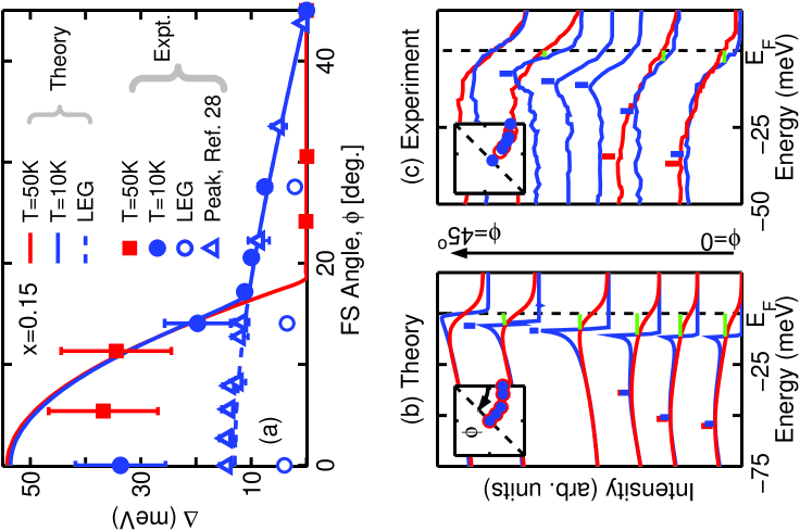
Figure 1: (color online) (a) Theoretical and experimental angle dependence of various gaps $\Delta$ in underdoped LSCO ($x$=0.15 ) along the FS, where $\phi=0$ denotes the antinodal and $\phi=45^{o}$ the nodal direction. Solid lines give our results for the normal ($T=50$K, red line) and the superconducting state ($T=10$K, blue line), and the corresponding experimental data are plotted with filled symbols of the same colorterashima . Blue dashed line shows the computed leading edge gap (LEG) at $T=10$K, while blue open circles give the corresponding experimental LEG as discussed in the text. Blue open triangles denote $\Delta$ based on peak positions from the data of Ref. mesot2, . (b) Computed energy distribution curves (EDCs) at different momentum points along the FS (see inset) for the normal ($T=50$K, blue lines) and the SC state ($T=10$K, red lines). Spectra at the bottom of the figure refer to the antinodal direction ($\phi=0$), while those at the top to the nodal direction ($\phi=45^{o}$). Blue and red tick marks on the spectra denote total gap values while green lines mark the LEG. (c) Same as (b), except that this figure refers to the experimental EDCs taken from Figs. 2(a) and (b) of Ref. terashima, . In order to highlight spectral changes, normal state spectra (red) are plotted on top of those for the SC state (blue) in several cases, even though these pairs of spectra are not taken at exactly the same angle $\phi$.

ARPES experiments in underdoped LSCO report two strikingly different angle dependencies of the gap,terashima ; mesot2 but find a natural explanation within our approach. Our calculations for underdoped LSCO ($x=0.15$) are shown in Fig. 1(a)-(c). In this case, our self-consistent solution yields a staggered magnetization of $S=0.21$, which increases very weakly with $T$ up to $T_{c}$. The SC gap, i.e. $\Delta(T=0)$ is 13meV with $T_{c}=48$K, which is higher than the experimental value of 37Kterashima , reflecting presumably the neglect of phase fluctuationsemery in our mean field treatment. Interestingly, although the computed ratio $2\Delta/k_{B}T_{c}=6.3$ is anomalously large, it is in good agreement with experimentswangdelta .

We consider first the theoretical results in Figs. 1(a) and (b). Fig. 1(a) displays calculated and experimental gap values along the Fermi surface as a function of the angle $\phi$ (inset to Fig. 1(b)), where $\phi=0$ corresponds to the antinodal direction, and $\phi=45^{o}$ to the nodal direction. Focusing on the energy distribution curves (EDCs) of the normal state (red spectra) in (b), the pseudogap appears as a broad hump feature with a large gap in the antinodal direction ($\phi=0$) as marked by red tick marks, which decreases to zero by $\phi=18^{o}$. For $\phi$ values between $18^{o}$ and $45^{o}$, the FS contains an ungapped nodal pocket or a FS arc (red curve in (a)). Below $T_{c}$, the EDCs (blue spectra) show an additional sharp peak and a leading edge superconducting gap (LEG) over the whole FS as marked by green lines, while the hump feature (blue tick marks) remains in the antinodal region. The presence of a peak-dip-hump feature in the SC state clearly reflects the two gap behavior, where the peak follows a simple $d-$wave form while the hump traces the pseudogap. Note that all theoretical spectra in (b) have been broadened by incorporating the effect of small angle scattering on the quasiparticlestanmoy ; see Appendix B for details. This allows the development of a finite spectral weight at $E_{F}$ and the formation of the leading edge gap, even though the underlying quasiparticle states lie well below $E_{F}$ at most momentascbroad .

The theoretically predicted gaps derived from the normal and SC state spectra of Fig. 1(b) are plotted in Fig. 1(a), and show good agreement with the corresponding experimental data. The characteristics of the evolution of the theoretical spectra with FS angle in the presence of two gaps, and how these spectra differ between the normal and the SC state, as discussed above in connection with Fig. 1(b), are also seen in the experimental spectraterashima of Fig. 1(c). In particular, our theoretical prediction that the gap is a pure SC gap up to the tip of the FS arc around $\phi=18^{o}$ (see (a)), but that it crosses over into becoming a total gap composed of SC and pseudogap thereafter, gives insight into various experimental results reported in the literatureterashima ; mesot2 . The peak plotted by Shi et. al.mesot2 corresponds to our calculated SC peak, and as shown in Fig. 1(a) (blue triangles), this gap displays a simple $d-$wave form. In contrast, Terashima et. al.terashima consider the hump feature and the associated data show a two-gap behavior (blue dots in (a)). Nevertheless, in the latter dataterashima which is reproduced in (c), the presence of the $d-$wave LEG can be seen. We have obtained values of the LEG from the spectra in (c) and plotted these as open circles in (a). A similar two-gap behavior can be seen even more clearly in (Bi,Pb)₂(Sr,La)₂CuO_6+δ (Bi2201) data in Fig. 3 of Ref. kondo, .

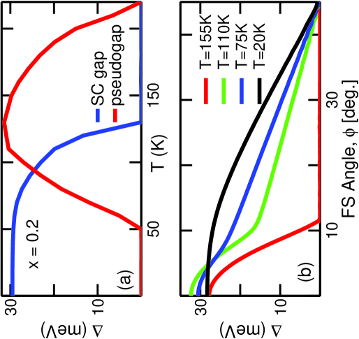
Figure 2: (color online) Self-consistently computed results for LSCO at $x=0.20$.uv (a) Temperature dependence of the SC gap (blue line) and the pseudogap (red line) showing reentrant behavior discussed in the text. (b) Angle dependence of the gap at different temperatures.

In the underdoped region, the pseudogap is large compared to the SC gap. The pseudogap increases weakly with $T$ while the SC gap decreases with $T$. This results in a nearly constant total gap $\Delta=\sqrt{\Delta_{AFM}^{2}+\Delta_{SC}^{2}}$, which is consistent with experimental observationskanigel . But at higher dopings, where the size of the SC gap becomes comparable to that of the pseudogap, a more interesting temperature dependence can emerge as seen in Fig. 2(a). Here a pseudogap is present at high temperature, but after the SC gap turns on at 130K,foot3 the pseudogap is suppressed to zero at 50K and thereafter the total gap becomes a pure SC gap. This leads to the evolution of the angle dependence of $\Delta$ shown in Fig. 2(b). At low temperature ($T=20$K, black line), the gap is pure $d-$wave, but at high temperature ($T=155$K, red line), it is a pure pseudogap, and at intermediate temperatures the gap shows a two-gap behavior similar to that of Fig. 1(a). Such a transition from a pure $d-$wave pairing gap to a pure pseudogap through a region in which both gaps coexist has recently been observed in ARPES measurementszxshen ; kanigel on Bi2212 above the optimal doping region. The crossover to pure $d-$wave form at low temperatures has been taken as evidence that the pseudogap is a precursor SC gap. In contrast, our analysis demonstrates that the appearance of a pure $d-$wave form at low temperatures can simply be the replacement of one kind of order by a more stable competitor.

Very different temperature and angle-dependencies in the underdoped vs optimal/overdoped regions discussed above can be readily understood. The pseudogap, which originates here from an ordered phase, only partially gaps the FS at any finite doping $x$. The SC gap, on the other hand, opens everywhere, except at the nodal points, so that if superconductivity is strong enough it can quench a preexisting ordered pseudogapbilbro . While it is natural to take the competing order to be an SDW in electron-doped cuprates, where long-range Néel order persists up to optimal doping, the choice is less clear for hole-doping. Accordingly, in Section IV below, we explore other choices for the pseudogap.

III Two Gap Scenario and the STM Data

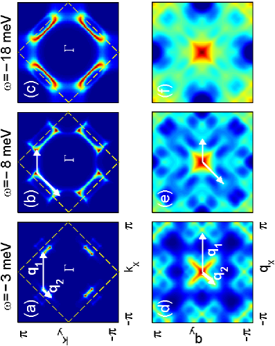
Figure 3: (color online) (a)-(c) Spectral intensity at different energies $\omega$ below $E_{F}$. Yellow dashed lines mark the magnetic zone boundary. (d)-(f) Corresponding simulated $q-$maps obtained by convoluting the maps (a)-(c), plotted on a log-scale to highlight weak features. Scattering vectors ${\bf{q}}_{1}$ and ${\bf{q}}_{2}$, shown by arrows, are discussed in the text. Red color denotes the highest and blue the lowest intensity.

We turn next to discuss STM results, where also a two-gap behavior has been reported recentlyhoffman ; mcelroy ; hanaguri ; fujita ; davis . In STM one measures the so-called $q-$map, from which the underlying FS and the angle-dependence of the gap can be extracted by interpreting the $q-$map as the Fourier transform of a quasiparticle interference (QPI) patternhoffman ; mcelroy . Figure 3 analyzes the relationship between $q-$maps and the one-particle spectral weights within our model, where the spectral weights characterize the ARPES spectra to the extent that the ARPES matrix elementbansil can be neglected. The computations are based on the LSCO parameters of Fig. 1 for $x=0.15$ at $T=10$K. In Figs. 3(a)-(c), the computed spectral weight $A({\bf{k}},\omega)$ is seen to reside mostly in the momentum region of ‘bananas’ or ‘arcs’ below the AFM zone boundaryfooteh . At low $\omega$ the spectral weight is further concentrated in two bright red spots at the ‘tips’ of each banana, but at higher energies the weight spreads out more uniformly over the whole FS arc as seen for example in Fig. 3(c). The corresponding $q-$maps, modeled as a convolution of the spectral intensity, i.e. $I_{\bf{q}}=\sum_{\bf{k}}A({\bf{k}},\omega)A({\bf{k}}+{\bf{q}},\omega)$, are shown in Figs. 3(d)-(f), and display intense peaks at the special $q-$vectors, which connect the bright spots in $A({\bf{k}},\omega)$hanaguri . Two such vectors ${\bf{q}}_{1}$ and ${\bf{q}}_{2}$ are marked in several panels in Fig. 3 as examplesfoot2 . It is striking that at high energy in (c), when the bright tips of bananas in $A({\bf{k}},\omega)$ have essentially disappeared, the $q-$map in (f) more or less loses its pattern of well defined peaks as the intensity spreads out over a wide region.

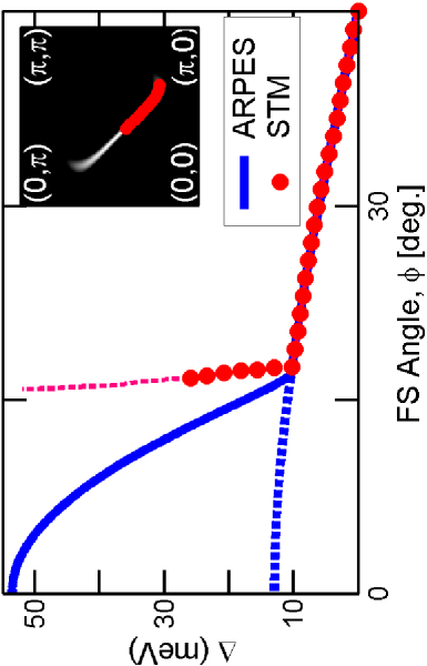
Figure 4: (color online) Apparent gap $\Delta$ as a function of the FS angle (red dots) as obtained from an analysis of the simulated $q-$maps of Figs. 3(d)-(f). Along the red dashed line the peaks in the $q-$maps are quite broad and may be hard to see experimentally. Blue solid line, which gives the total gap, as well as the dashed blue line giving the SC gap, is reproduced from Fig. 1(a) for reference. Inset: White trace depicts the normal state FS on which the FS points obtained from the analysis of $q-$maps of Figs. 3(d)-(f) are shown as red dots.

The simulated $q-$maps of Figs. 3(d)-(f) can be used to reconstruct the pattern of bright spots in Figs. 3(a)-(c), and to thus obtain the FS and the angle-dependent gap, as is done commonly in analyzing STM data. The resulting gap $\Delta$ is seen from Fig. 4 (red dots) to yield the SC gap in accord with the ARPES data (blue solid line), but only up to approximately the edge of the FS arc. Interestingly, for higher $\omega$’s, ARPES follows the pseudogap up to the edge of the Brillouin zone boundary at $\phi=0$ (blue solid line), but the STM-derived gaps remain within the AFM boundary up to the end of the FS arc at $\phi=18^{o}$. As a result the apparent STM gap adduced from the $q-$map shoots up nearly vertically at $\phi=18^{o}$ following the red dashed line. But with increasing energy above the maximum of the SC gap of 13meV at $\phi=0$, it becomes difficult to extract $\Delta$ values as the $q-$map gradually loses its well defined peak pattern except at $q=0$. Note also that the FS points deduced from the $q-$maps stop near the AFM zone boundary (see inset to Fig. 4). These key characteristics of the FS and the angle-dependence of the gap in Fig. 4 are in remarkable accord with the behavior reported in a recent STM study of Bi2212davis , and reflect the effect of loss of structure in $q-$maps with increasing energy, which was pointed out above in connection with Fig. 3.

IV CDW, DDW and other Orders

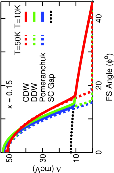
Figure 5: (color online) Computed angle dependence of the gap $\Delta$ in the normal (solid lines) and superconducting state (dashed lines) for various competing orders: CDW (red lines); DDW (green lines); and Pomeranchuk instability for one axis, which is taken to be the $y$ axis (blue lines). Black dotted line gives the pure $d-$wave gap in the absence of any other competing order.

Although we have focused on properties of the SDW state in this article, we have also carried out calculations on a number of other competing electron-hole ordered phases, including the CDW, the DDW, and the Pomeranchuk mode; see Appendix C for technical details. Fig. 5, which summarizes our key results, shows that the CDW (red lines) and DDW (green lines) orders with the same reduced AFM Brillouin zone as the SDW, yield a gap symmetry very similar to that of Fig. 1 in the normal as well as the superconducting state. A doped spin liquid model for the pseudogapvalenzuela gives similar results. However, a Pomeranchuk modemarkiephase ; yamase does not show a true gap, but splits the van Hove singularity (VHS) along $x$ and $y$ axes. We can, however, obtain two-gap results similar to those of Fig. 1, along one axis, as shown by the blue lines in Fig. 5, suggesting that in a multi-domain sample it might be hard to distinguish this behavior from the experimental two-gap data. Finally, we have studied a linear antiferromagnetic (LAFM) phasemarkielafm , which has a one-dimensional ordering vector ($\pi,0$), as might be seen in a stripe phase. However, we find that the resulting two gap structure displays a very different symmetry pattern, which is not consistent with experiments.

V Arcs vs Pockets

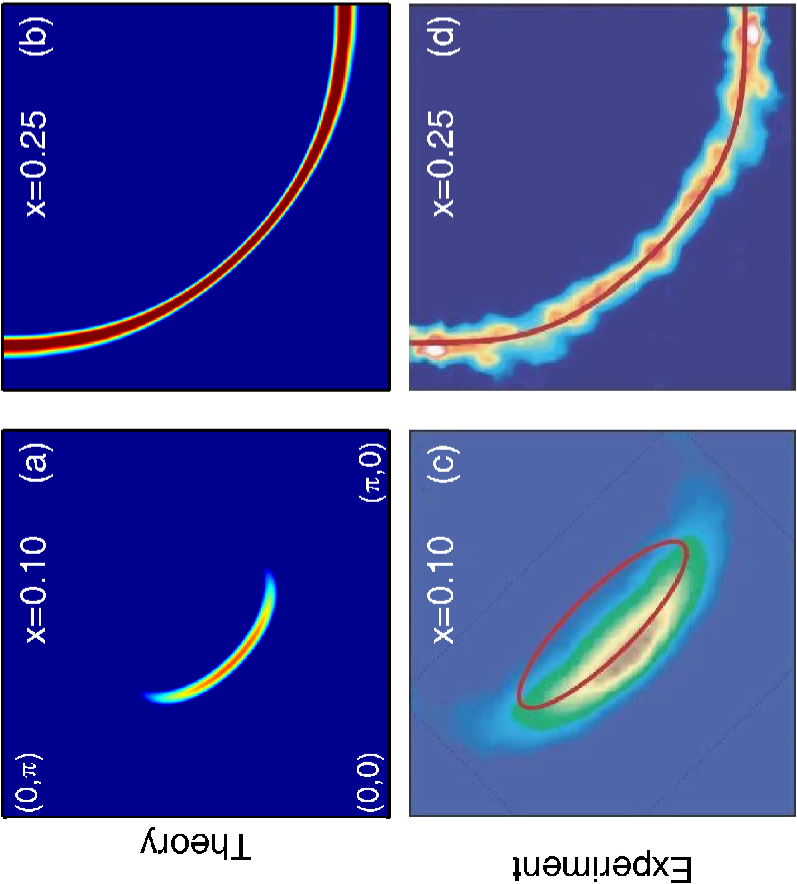
Figure 6: (color online) (a)-(b) Computed Fermi surface maps for Na-CCOC based on the AFM model at $x=0.10$ and $x=0.25$. Tight binding model parameters used in the calculations are: $t=126$, $t^{\prime}=-36$, $t^{\prime\prime}=10$ meV, with $U=4.5t$ for $x=0.1$ (gives $S=0.3$) and $U=3.2t$ for $x=0.25$ (gives $S=0$). (c)-(d) After Ref. leyraud, , where the FS’s obtained in Na-CCOC via ARPES from Ref. ccoc, are shown. Red line in (c) depicts the FS of YBCO adduced from Shubnikov-de Haas experiments of Ref. leyraud, at similar doping levels.

An important issue is whether experiments see a well-defined pocket or merely a Fermi arc. The recent Shubnikov-de Haas (SdH) experiments find oscillations in underdoped YBa₂Cu₃O_6.5 and YBa₂Cu₄O₈ (YBCO) and argue for the presence of a closed pocket of approximately the expected sizeleyraud ; yelland ; bangura . Note that the AFM model clearly predicts a full pocket, but the calculated spectral weight resembles the Fermi arc with little intensity on the shadow side due to the effect of AFM coherence factors [see Figs. 3(a)-(c) and the inset to Fig. 4]. Fig. 6 shows results based on the AFM model for another hole doped cuprate, Ca_2-xNa_xCuO₂Cl₂ (Na-CCOC)ccoc . In the underdoped system at $x=0.10$, areas of the possible FS pocket in Na-CCOC and YBCO would be similar.leyraud While the observed pocket in YBCO (red line in (c)) is somewhat too smallfoot4 to satisfy Luttinger’s theorem, it should be remembered that YBCO has a bilayer splitting which unlike Bi2212 is not small in the nodal direction. Hence two nodal FS pockets are expected, where the smaller pocket is presumably easier to observe in a quantum oscillation experiment.foot5 Finally, we note that ARPES data from underdoped LSCO has recently detected weak spectral weight on the shadow side of the nodal pocket$-$ see Fig. 2 of Ref. yoshida, for doping $x=0.03$, and $0.07$. Interestingly, Kaul et al.Kaul point out that this shadow is consistent with a conventional AFM metal, but it is not expected in the exotic holon metal phase.

VI Electron vs hole doping

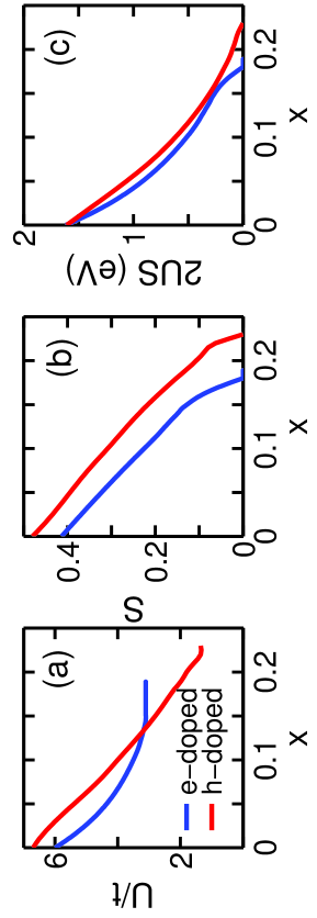
Figure 7: (color online) Comparison of selected parameters for electron-doped NCCO/PCCO tanmoysns (blue lines) vs hole-doped LSCO (red lines). (a) Effective interaction $U/t$; (b) Self-consistent magnetisation $S$; and, (c) Total AFM gap $2US$.

The question of electron-hole symmetry has been a topic of interest in cuprate physics for some time. The magnetic properties display a strong asymmetrydamascelli02 in that long-range AFM order persists up to optimal doping with electron doping, but it disappears at quite low doping levels in the hole doped case as it is replaced by the mysterious pseudogap phase. Moreover, nanoscale phase separation, which is prominent in hole-doped cuprates, seems to be largely absent in electron doped materialsAAPH . Some of these differences could be understood in terms of how the magnetic susceptibility evolves with electron vs hole doping.MKII ; water3

The electronic properties, on the other hand, appear to show greater symmetry in that superconductivity arises near a possible quantum critical point (QCP) close to optimal doping, which is associated with a crossover from small to large Fermi surface (FS)nparm ; Balak . In this connection, Fig. 7 compares the doping dependencies of selected parameters within the AFM model in electron doped Nd_2-xCe_xCuO₂ (NCCO) and Pr_2-xCe_xCuO₂ (PCCO) (blue lines) and hole doped LSCO (red lines). Here, parameters for electron doping are taken from our earlier worktanmoysns . The effective $U$ in Fig. 7(a) decreases almost linearly with doping in the very underdoped region in a very similar manner for both electron and hole doping. At higher doping, the smaller $U$ found for hole doping could be associated with larger screening resulting from the proximity of the VHS. The self-consistently calculated value of the staggered magnetization $S$, however, remains higher than that on the electron doped side over the entire doping range as seen in Fig. 7(b). Remarkably, the total AFM gap $2US$ ($t=0.326$ eV for electron doping) displays electron-hole symmetry, although the QCP is slightly higher for hole doping.

The effect of the VHS is reflected in the superconducting properties as well. At $x=0.15$, for example, the self-consistently calculated values of the superconducting order parameters are as follows: for electron (hole) doping, $V=-134(-78.4)$ meV and $\Delta=2.6(13)$ meV. That is, even though the interaction $V$ is much weaker for the hole-doped case, the SC gap is found to be larger, leading to a larger ratio $2\Delta/k_{B}T_{c}$ of 6.3 for hole doping compared to 4.1 for electron doping.

In the electron-doped cuprates the QCP involves two topological transitions as a function of doping. At low doping, the FS consists of electron pockets near $\Gamma$. As doping increases, a second hole-like pocket emerges along the nodal direction around 15% doping (in NCCO) as the magnetic gap decreases and the lower magnetic band crosses the Fermi level. The appearance of this pocket can be detected in ARPES, Hall effect, and penetration depth measurements at essentially the same doping leveltanmoysns . At higher doping, the gap collapses and the FS evolves into a single large hole-like sheet. A reverse scenario seems to be followed for hole doping: A nodal hole-like FS pocket is present at the lowest dopings (corresponding to the Fermi arc), while at higher dopings Hall effect evidence has been foundBalak for the appearance of electron-like pockets in Bi2201, again at approximately 15% doping. In our model, these would be the $\Gamma$-centered electron pockets associated with the upper magnetic band.

VII Conclusion

In conclusion, our model calculations show that most of the characteristic features observed in ARPES as well as STM two-gap studies are consistent with a scenario in which the pseudogap has a non-superconducting origin in a competing phase. In contrast, a precursor superconductor model of the pseudogap will have difficulties explaining why the higher order harmonic content of the gap grows with increasing temperature as seen in Fig. 2. Our computed spectra not only show the presence of a feature which scales with the pseudogap, but also display a superconducting low-energy gap leading to a peak-dip-hump structure. As doping increases toward the quantum critical point of the pseudogap, we find that a region of reentrant superlattice order could reappear in the system. Our analysis highlights electron-hole symmetry of electronic properties of the cuprates, even though the magnetic properties are well-known to be quite asymmetric.

Appendix A Model for the coexistence of SDW and $d-$SC orders

Models of competing SDW and SC order have been studied for many yearsmachida ; gabovich ; bilbro . In our calculations, we use a one band tight binding model Hamiltonian where antiferromagnetism is included via a Hubbard $U$ and superconductivity as in the BCS theory:tanmoy

$$H = \sum_{\vec{k},\sigma}\xi_{\vec{k}}c_{\vec{k},\sigma}^{{\dagger}}c_{\vec{k},\sigma}+U\sum_{\vec{k},\vec{k^{\prime}}}c_{\vec{k}+\vec{Q},\uparrow}^{{\dagger}}c_{\vec{k},\uparrow}c_{\vec{k^{\prime}}-\vec{Q},\downarrow}^{{\dagger}}c_{\vec{k}^{\prime},\downarrow}$$ (1)

$$+\sum_{\vec{k},\vec{k^{\prime}}}V(\vec{k},\vec{k^{\prime}})c_{\vec{k},\uparrow}^{{\dagger}}c_{-\vec{k},\downarrow}^{{\dagger}}c_{-\vec{k^{\prime}},\downarrow}^{{\dagger}}c_{\vec{k}^{\prime},\uparrow}^{{\dagger}},$$

where $c_{\vec{k},\sigma}^{{\dagger}}(c_{\vec{k},\sigma})$ is the electronic creation (destruction) operator with momentum $\vec{k}$ and spin $\sigma$ ($\bar{\sigma}$ is the opposite spin). The bare particle dispersion with respect to the chemical potential $E_{F}$ is given by

$$\xi_{\vec{k}}=-2t[c_{x}(a)+c_{y}(a)]-4t^{\prime}c_{x}(a)c_{y}(a)$$

$$~{}~{}~{}~{}~{}~{}-2t^{\prime\prime}[c_{x}(2a)+c_{y}(2a)]$$

$$~{}~{}~{}~{}~{}~{}-4t^{\prime\prime\prime}[c_{x}(2a)c_{y}(a)+c_{x}(a)c_{y}(2a)]-E_{F},$$ (2)

with $c_{i}(\alpha a)=cos(\alpha k_{i}a)$ and $a$ being the lattice constant. $t,t^{\prime},t^{\prime\prime}$ and $t^{\prime\prime\prime}$ are TB hopping parameters. Defining the Nambu operator in the magnetic Brillouin zone (MBZ)

$$\Psi_{\vec{k}}=\left(\begin{array}[]{c}c_{\vec{k},\uparrow}\\ ~{}~{}~{}c_{\vec{k}+\vec{Q},\uparrow}\\ ~{}c_{-\vec{k},\downarrow}^{{\dagger}}\\ ~{}~{}~{}~{}c_{-\vec{k}-\vec{Q},\downarrow}^{{\dagger}}\end{array}\right)$$ (3)

we can write the above Hamiltonian in the MBZ as

$$H=\left(\begin{array}[]{ccccc}~{}\xi_{\vec{k}}&-US&~{}\Delta_{\vec{k}}&~{}0\\ -US&~{}\xi_{\vec{k}+\vec{Q}}&~{}0&~{}~{}\Delta_{\vec{k}+\vec{Q}}\\ ~{}\Delta_{\vec{k}}&0&-\xi_{\vec{k}}&-US\\ ~{}0&~{}\Delta_{\vec{k}+\vec{Q}}&-US&~{}-\xi_{\vec{k}+\vec{Q}}\end{array}\right)$$ (4)

where the order parameters $S$ and $\Delta_{\vec{k}}$ represent the staggered magnetization at nesting vector $\vec{Q}=(\pi,\pi)$ and the superconducting gap, respectively. In the mean field approximation, these are defined by

$$S = \sum_{\vec{k},\sigma}\sigma\left\langle c_{\vec{k}+\vec{Q},\sigma}^{{\dagger}}c_{\vec{k},\sigma}\right\rangle,$$ (5)

$$\Delta_{\vec{k}} = \sum_{\vec{k^{\prime}}}V(\vec{k},\vec{k^{\prime}})\left\langle c_{\vec{k^{\prime}},\uparrow}^{{\dagger}}c_{-\vec{k^{\prime}},\downarrow}^{{\dagger}}\right\rangle=\Delta g_{\vec{k}}$$ (6)

$$= Vg_{\vec{k}}\sum_{\vec{k^{\prime}}}g_{\vec{k^{\prime}}}\left\langle c_{\vec{k^{\prime}},\uparrow}^{{\dagger}}c_{-\vec{k^{\prime}},\downarrow}^{{\dagger}}\right\rangle=-\Delta_{\vec{k}+\vec{Q}},$$

where the $d_{x^{2}-y^{2}}-$orbital phase factor is $g_{\vec{k}}=[c_{x}(a)-c_{y}(a)]/2$. We diagonalize the Hamiltonian of Eq. 4 by the Bogolyubov method and the corresponding unitary matrix can be easily constructedzaira ,

$$\hat{U}_{\vec{k},\sigma}=\left(\begin{array}[]{cccc}\alpha_{\vec{k}}u^{+}_{\vec{k}}&\sigma\beta_{\vec{k}}u_{\vec{k}}^{-}&-\alpha_{\vec{k}}v_{\vec{k}}^{+}&\sigma\beta_{\vec{k}}v^{-}_{\vec{k}}\\ -\sigma\beta_{\vec{k}}u^{+}_{\vec{k}}&\alpha_{\vec{k}}u_{\vec{k}}^{-}&\sigma\beta_{\vec{k}}v_{\vec{k}}^{+}&\alpha_{\vec{k}}v^{-}_{\vec{k}}\\ \alpha_{\vec{k}}v^{+}_{\vec{k}}&-\bar{\sigma}\beta_{\vec{k}}v_{\vec{k}}^{-}&\alpha_{\vec{k}}u_{\vec{k}}^{+}&\bar{\sigma}\beta_{\vec{k}}u^{-}_{\vec{k}}\\ -\bar{\sigma}\beta_{\vec{k}}v^{+}_{\vec{k}}&-\alpha_{\vec{k}}v_{\vec{k}}^{-}&-\bar{\sigma}\beta_{\vec{k}}u_{\vec{k}}^{+}&\alpha_{\vec{k}}u^{-}_{\vec{k}}\\ \end{array}\right).$$ (7)

The Bogolyubov coefficients are chosen to be

$$\alpha_{\vec{k}}(\beta_{\vec{k}}) = \frac{1}{2}\sqrt{1\pm\frac{\xi_{\vec{k}}^{-}}{E_{0\vec{k}}}}$$ (8)

$$u_{\vec{k}}^{\nu}(v_{\vec{k}}^{\nu}) = \frac{1}{2}\sqrt{1\pm\frac{\xi_{\vec{k}}^{+}+\nu E_{0\vec{k}}}{E^{\nu}_{\vec{k}}}},$$ (9)

where $\xi_{\vec{k}}^{\pm}=(\xi_{\vec{k}}\pm\xi_{\vec{k}+\vec{Q}})/2$ and $E_{0\vec{k}}=\sqrt{(\xi_{\vec{k}}^{-})^{2}+(US)^{2}}$. The four resulting quasiparticle bands have energies $\pm E^{+}_{\vec{k}}$, $\pm E^{-}_{\vec{k}}$, where

$$(E^{\nu}_{\vec{k}})^{2}=(\xi_{\vec{k}}^{+}+\nu E_{0\vec{k}})^{2}+\Delta_{\vec{k}}^{2},$$ (10)

and $\nu=\pm$ refers to the upper (+) and lower (-) magnetic bands (U/LMB). The $4\times 4$ Matsubara Green’s function can be defined from the Nambu operator as $G(\vec{k},\tau-\tau^{\prime})=-\left\langle T_{\tau}\Psi_{\vec{k}}(\tau)\Psi_{\vec{k}}^{{\dagger}}(\tau^{\prime})\right\rangle$, whose Fourier transformation gives,

$$G(\vec{k},\sigma,i\omega_{n})=\hat{U}_{\vec{k},\sigma}(i\omega_{n}-H_{\rm{diag}})^{-1}\hat{U}_{\vec{k},\sigma}^{{\dagger}}$$ (11)

where $H_{\rm{diag}}$ is the diagonalized Hamiltonian containing the eigenvalues in order $[E_{\vec{k}}^{+},E_{\vec{k}}^{-},-E_{\vec{k}}^{+},-E_{\vec{k}}^{-}]$. The corresponding $4\times 4$ spectral function is defined in the standard form $A(\vec{k},\sigma,i\omega_{n})=-{\rm{Im}}[G(\vec{k},\sigma,i\omega_{n})]/\pi$. We calculate the self-consistent values of various order parameters for each hole doping $x$, by simultaneously solving the following set of equations

$$x = 1-\sum_{\vec{k},\sigma}\int_{-\infty}^{\infty}\frac{d\omega}{2\pi}A_{11}(\vec{k},\sigma,\omega+i\delta)f(\omega),$$ (12)

$$S = \sum_{\vec{k},\sigma}\sigma\int_{-\infty}^{\infty}\frac{d\omega}{2\pi}A_{12}(\vec{k},\sigma,\omega+i\delta)f(\omega),$$ (13)

$${\rm{and}}$$

$$\Delta = V\sum_{\vec{k},\sigma}\int_{-\infty}^{\infty}\frac{d\omega}{2\pi}A_{13}(\vec{k},\sigma,\omega+i\delta)f(\omega).$$ (14)

$f(\omega)=1/(\exp{(\omega/k_{B}T)}+1)$ is the Fermi function at temperature $T$ where $k_{B}$ is the Boltzmann constant.

Appendix B Broadening due to small angle scattering

In both ARPES and STM calculations we model the large spectral broadening to be due to elastic small angle scattering of the Cooper pairs (neglecting pair breaking effects), in which case the Green’s function remains of the same form but with renormalized parameters $\omega\rightarrow\tilde{\omega}=\omega Z_{\vec{k}}(\omega)$ and $\Delta_{\vec{k}}\rightarrow\tilde{\Delta}_{\vec{k}}=\Delta_{\vec{k}}Z_{\vec{k}}(\omega)$. The renormalization factor is taken to befoot1 ,

$$Z_{\vec{k}}(\omega)=1+\frac{i\Sigma_{\vec{k}}(\omega)}{\sqrt{\omega^{2}-\Delta_{\vec{k}}^{2}}},$$ (15)

where $\Sigma_{\vec{k}}(\omega)$ is the self energy correction due to impurity scattering, which is related to the normal state scattering rate astanmoy

$$\Sigma_{\vec{k}}(\omega)={\rm{sgn}}(\omega)(C_{0}+C_{1}\omega^{p}).$$ (16)

The power $p=3/2$ is assumed to apply for holes, as found for electron doped cupratestanmoy . The other parameters $C_{0}$ and $C_{1}$ are found by fitting to the experimental broadening. For ARPES calculations $C_{0}=C_{1}=50$meV. For STM, the $\omega-$dependence is neglected and $C_{0}=30$meV.

Appendix C Other models of competing order

We have also studied various other ordered phases such as the CDW, the DDW, the Pomeranchuk instability, and the linear antiferromagnetism (LAFM). All these orders possess the same superlattice behavior and/or the pseudospin character near the Van Hove singularity and thus are possible candidates for the origin of the pseudogap. When the Hamiltonian is solved in the mean field approximation, the eigenvalues are similar to Eq. 10 for SDW except that $E_{0\vec{k}}$ is different for each phase.markiephase ; markielafm Defining the interaction as $V_{i}$ with $i=\rm{CDW,DDW,Pom,LAFM}$, $E_{0}$ can be written as

$$E_{0\vec{k}}=\sqrt{R_{x}^{2}+R_{y}^{2}+R_{z,\sigma}^{2}+(\xi_{\vec{k}}^{-})^{2}+2\xi_{\vec{k}}^{-}R_{x}},$$ (17)

where $R_{i}$ represent the gap in various phasesmarkiephase ; markielafm ; in Pomeranchuk mode $R_{x}=V_{\rm{Pom}}g_{\vec{k}}$, in DDW phase $R_{y}=V_{\rm{DDW}}g_{\vec{k}}$. In CDW and LAFM phase the gap is similar to the SDW phase except that in CDW the gap does not depend on the spin orientation of the system and thus $R_{z,\sigma}=V_{\rm{CDW}}$. The LAFM leads to a similar result, with $R_{z,\sigma}=\sigma V_{\rm{LAFM}}S$, except here the nesting of the FS occurs along $\vec{Q}=(\pi,0)$. In each case the interaction was adjusted to match the gap and the FS arc for LSCO at $x=0.15$ [see Fig. 5] The resulting values are $V_{\rm{DDW}}=200$, $V_{\rm{CDW}}=160$ meV, whereas in the Pomeranchuk mode, $R_{x}$ simply renormalizes $t$ to have unequal values of $x$ and $y$, $t_{x/y}=t\pm 1.2$ meV. We find that LAFM has the wrong pseudogap symmetry to explain the experiments.

References

- (1) Z.-X. Shen, D. S. Dessau, B. O. Wells, D. M. King, W. E. Spicer, A. J. Arko, D. Marshall, L. W. Lombardo, A. Kapitulnik, P. Dickinson, S. Doniach, J. DiCarlo, T. Loeser, and C. H. Park, Phys. Rev. Lett. 70, 1553 (1993); H. Ding, M. R. Norman, J. C. Campuzano, M. Randeria, A. F. Bellman, T. Yokoya, T. Takahashi, T. Mochiku and K. Kadowaki, Phys. Rev. B 54, 9678(R) (1996).
- (2) J. Mesot, M. R. Norman, H. Ding, M. Randeria, J. C. Campuzano, A. Paramekanti, H. M. Fretwell, A. Kaminski, T. Takeuchi, T. Yokoya, T. Sato, T. Takahashi, T. Mochiku, and K. Kadowaki, Phys. Rev. Lett. 83, 840 (1999).
- (3) M. Le Tacon, , A. Sacuto, A. Georges, G. Kotliar, Y. Gallais, D. Colson, and A. Forget, Nature Physics 2, 537 (2006).
- (4) M. Hashimoto, T. Yoshida, K. Tanaka, A. Fujimori, M. Okusawa, S. Wakimoto, K. Yamada, T. Kakeshita, H. Eisaki, and S. Uchida, Phys. Rev. B 75, 140503(R) (2007).
- (5) S. Huefner, M.A. Hossain, A. Damascelli, and G.A. Sawatzky, arXiv:0706.4282, and references therein.
- (6) W. S. Lee, I. M. Vishik, K. Tanaka, D. H. Lu, T. Sasagawa, N. Nagaosa, T. P. Devereaux, Z. Hussain, and Z.-X. Shen, Nature 450, 81 (2007).
- (7) A. Kanigel, M. R. Norman, M. Randeria, U. Chatterjee, S. Souma, A. Kaminski, H. M. Fretwell, S. Rosenkranz, M. Shi, T. Sato, T. Takahashi, Z. Z. Li, H. Raffy, K. Kadowaki, D. Hinks, L. Ozyuzer, and J. C. Campuzano, Nature Physics 2, 447 (2006); A. Kanigel, U. Chatterjee, M. Randeria, M. R. Norman, S. Souma, M. Shi, Z. Z. Li, H. Raffy, and J. C. Campuzano, Phys. Rev. Lett. 99, 157001 (2007).
- (8) Ch. Renner, B. Revaz, J.-Y. Genoud, K. Kadowaki, and O. Fischer, Phys. Rev. Lett. 80, 149 (1998).
- (9) T. Eckl and W. Hanke, Phys. Rev. B 74, 134510 (2006).
- (10) H.-H. Wen, and X.-G. Wen, Physica C 460, 28 (2007).
- (11) Tung-Lam Dao, Antoine Georges, Jean Dalibard, Christophe Salomon, and Iacopo Carusotto, Phys. Rev. Lett. 98, 240402 (2007).
- (12) Guy Deutscher, Nature 397, 410 (1999).
- (13) V. M. Krasnov, A. Yurgens, D. Winkler, P. Delsing, and T. Claeson, Phys. Rev. Lett. 84, 5860 (2000).
- (14) K. Tanaka, W. S. Lee, D. H. Lu, A. Fujimori, T. Fujii, Risdiana, I. Terasaki, D. J. Scalapino, T. P. Devereaux, Z. Hussain, and Z.-X. Shen, Science 314, 1910 (2006).
- (15) Takeshi Kondo, Tsunehiro Takeuchi, Adam Kaminski, Syunsuke Tsuda, and Shik Shin, Phys. Rev. Lett. 98, 267004 (2007).
- (16) K. Terashima, H. Matsui, T. Sato, T. Takahashi, M. Kofu, and K. Hirota, Phys. Rev. Lett. 99, 017003 (2007).
- (17) K. M. Shen, F. Ronning, D. H. Lu, F. Baumberger, N. J. C. Ingle, W. S. Lee, W. Meevasana, Y. Kohsaka, M. Azuma, M. Takano, H. Takagi, and Z.-X. Shen, Science 307, 901 (2005).
- (18) J. E. Hoffman,K. McElroy, D.-H. Lee, K. M Lang, H. Eisaki, S. Uchida, and J. C. Davis, Science 297, 1148 (2002).
- (19) K. McElroy, R. W. Simmonds, J. E. Hoffman, D.-H. Lee, J. Orenstein, H. Eisaki, S. Uchida, J. C. Davis, Nature 422, 592 (2003).
- (20) T. Hanaguri Y. Kohsaka, J. C. Davis, C. Lupien, I. Yamada, M. Azuma, M. Takano, K. Ohishi, M. Ono, H. Takagi, Nature Physics 3, 865 (2007).
- (21) J. C. Davis, Presented at Yamada Conference LXI on Spectroscopies in Novel Superconductors (SNS 2007), Sendai, Japan, August 2007 (unpublished).
- (22) Tanmoy Das, R.S. Markiewicz and A. Bansil, Phys. Rev. B 74, 020506(R) (2006).
- (23) Tanmoy Das, R.S. Markiewicz and A. Bansil, Phys. Rev. Lett. 98, 197004 (2007).
- (24) R.S. Markiewicz, Phys. Rev. B 70, 174518 (2004).
- (25) A. Comanac, L de Medici, M. Capone, and A. J. Millis, arXiv:0712.2392.
- (26) This set of TB parameters describes a wide variety of experiments, including ARPES dispersions and Fermi surfaces, closely describes LDA dispersion within an overall renormalization factor. R. S. Markiewicz, S. Sahrakorpi, M. Lindroos, Hsin Lin, and A. Bansil, Phys. Rev. B 72, 054519 (2005).
- (27) The values of the interaction potentials are and meV at . For , the parameters are chosen to illustrate the reentrance of the pseudogap as described in the text: and meV.
- (28) M. Shi, J. Chang, S. Pailh s, M. R. Norman, J. C. Campuzano, M. Mansson, T. Claesson, O. Tjernberg, A. Bendounan, L. Patthey, N. Momono, M. Oda, M. Ido, C. Mudry, and J. Mesot, arXiv:0708.2333.
- (29) V. J. Emery and S. A. Kivelson, Nature (London) 374, 434 (1995).
- (30) Yue Wang, Jing Yan, Lei Shan, Hai-Hu Wen, Yoichi Tanabe, Tadashi Adachi, and Yoji Koike, Phys. Rev. B 76, 064512 (2007); R. Khasanov, A. Shengelaya, A. Maisuradze, F. La Mattina, A. Bussmann-Holder, H. Keller, and K. A. Müller, Phys. Rev. Lett. 98, 057007 (2007).
- (31) The SC gap, however, has not been broadened.
- (32) The mean-field results should be compared to the short-range ordering temperature. In optimally doped LSCO, SC fluctuations turn on at K. See Yayu Wang, Lu Li, and N. P. Ong, Phys. Rev. B 73, 024510 (2006).
- (33) G. Bilbro and W. L. McMillan, Phys. Rev. B 14, 1887 (1976); C. A. Balseiro and L. M. Falicov, Phys. Rev. B 20, 4457 (1979).
- (34) K. Fujita, Ilya Grigorenko, J. Lee, M. Wang, Jian Xin Zhu, J.C. Davis, H. Eisaki, S. Uchida, and Alexander V. Balatsky, arXiv:0709.0632.
- (35) A. Bansil and M. Lindroos, Phys. Rev. Lett. 83, 5154 (1999).
- (36) We find a small electron-hole asymmetry in the -maps.
- (37) The point we call () is labelled as () in Ref. hoffman, and as () in Ref. mcelroy, .
- (38) B. Valenzuela and E. Bascones, Phys. Rev. Lett. 98, 227002 (2007).
- (39) R. S. Markiewicz and C Kusko, Phys. Rev. B. 66, 024506 (2002).
- (40) Hiroyuki Yamase, Phys. Rev. Lett. 93, 266404 (2004).
- (41) R. S. Markiewicz, and C Kusko, Phys. Rev. B 65, 064520 (2002).
- (42) N. Doiron-Leyraud, C. Proust, D. LeBoeuf, J. Levallois, J.-B. Bonnemaison, R. Liang, D.A. Bonn, W.N. Hardy, and L. Taillefer, Nature, 447, 565 (2007).
- (43) K.M. Shen, F. Ronning, D.H. Lu, F. Baumberger, N.J.C. Ingle, W.S. Lee, W. Meevasana, Y. Kohsaka, M. Azuma, M. Takano, H. Takagi, and Z.-X. Shen, Science 307, 901904 (2005).
- (44) E. A. Yelland, J. Singleton, C. H. Mielke, N. Harrison, F. F. Balakirev, B. Dabrowski, and J. R. Cooper, Phys. Rev Lett. 100, 047003 (2008).
- (45) A. F. Bangura, J. D. Fletcher, A. Carrington, J. Levallois, M. Nardone, B. Vignolle, P. J. Heard, N. Doiron-Leyraud, D. LeBoeuf, L. Taillefer, S. Adachi, C. Proust, and N. E. Hussey, Phys. rev. Lett. 100, 047004 (2008).
- (46) In an AFM model, the observed oscillation should correspond to two pockets associated with inequivalent nodal points.
- (47) A model involving slow antiferromagnetic fluctuations with a short correlation length in the spirit of the present AFM model has been invoked recently to explain the quantum oscillation data on YBCO: N. Harrison, R.D. McDonald, and J. Singleton, Phys. Rev. Lett. 99, 206406 (2007).
- (48) T. Yoshida, X.J. Zhou, K. Tanaka, W.L. Yang, Z. Hussain, Z.-X. Shen, A. Fujimori, S. Sahrakorpi, M. Lindroos, R.S. Markiewicz, A. Bansil, S. Komiya, Y. Ando, H. Eisaki, T. Kakeshita, and S. Uchida, Phys. Rev. B 74, 224510 (2006).
- (49) R.K. Kaul, Y.B. Kim, S. Sachdev, and T. Senthil, Nature Physics 4, 28 (2008).
- (50) Tanmoy Das, R.S. Markiewicz and A. Bansil, Yamada Conference LXI on Spectroscopies in Novel Superconductors (SNS 2007), Sendai, Japan, August 2007, arXiv:0711.1504.
- (51) A. Damascelli, Z.-X. Shen, and Z. Hussain, Rev. Mod. Phys. 75, 473 (2003).
- (52) M. Aichhorn, E. Arrigoni, M. Potthoff, and W. Hanke, Phys. Rev. B 74, 235117 (2006).
- (53) R.S. Markiewicz, S. Sahrakorpi, and A. Bansil, Phys. Rev. B 76, 174514 (2007).
- (54) N.P. Armitage, F. Ronning, D.H. Lu, C. Kim, A. Damascelli, K.M. Shen, D.L. Feng, H. Eisaki, Z.-X. Shen, P.K. Mang, N. Kaneko, M. Greven, Y. Onose, Y. Taguchi, and Y. Tokura, Phys. Rev. Lett. 88, 257001 (2002).
- (55) F.F. Balakirev, J.B. Betts, A. Migliori, I. Tsukada, Y. Ando, and G.S. Boebinger, arXiv:0710.4612.
- (56) K. Machida, J. Phys. Soc. Jpn. 50, 2195 (1981); J. Phys. Soc. Jpn., 52, 1333 (1983) and the references therein.
- (57) A.M. Gabovich, and A.I. Voitenko, Phys Rev B 75, 064516 (2007).
- (58) Z. Nazario, and D.I. Santiago, Phys. Rev. B 70, 144513 (2004).
- (59) R.S. Markiewicz, Phys. Rev. B 69, 214517 (2004).