Monte Carlo simulations of star clusters with primordial binaries. Comparison with $N$-body simulations and observations

Abstract

We outline the steps needed in to calibrate the Monte Carlo code in order to perform large scale simulations of real globular clusters. We calibrate the results against $N$-body simulations for $N=2500$, $10000$ and for the old open cluster M67. The calibration is done by choosing appropriate free code parameters.

1 Introduction

Most of the modeling of individual star cluster has been focused on static models based on the King model (see Meylan & Heggie 1997). There have been also a small number of studies able to follow the dynamical evolution of a system. They were mainly based on variants of a Fokker-Planck technique and small $N$-body simulations (e.g. Grabhorn et al.  1992, Drukier 1993, Murphy et al. 1998, Giersz & Heggie 2003 and Hurley et al.  2005).

In this presentation we show the further developments of the Monte Carlo code needed to properly follow the evolution of real star clusters. The dynamical ingredients of the code are basically the same as those described in Giersz (2006 and references therein). This code is based on an original code by Stodółkiewicz (1986), which in turn was based on the code devised by Hénon (1971). The extensions to the code were mainly connected with: (i) upgrading the prescription of stellar evolution to the algorithm of Hurley et al. (2000), (ii) adding the procedures for the internal evolution of binary stars (Hurley et al. 2002), both using the McScatter interface (Heggie, Portegies Zwart & Hurley 2006), (iii) a better treatment of the escape process in the presence of a static tidal field. Then the new version of the code was calibrated against the results of $N$-body simulations so as to allow us to construct dynamical evolutionary models of real star clusters.

2 The calibration of the Monte Carlo technique

For Monte Carlo simulations the standard $N$-body units are adopted. The unit of time, however, is proportional to $N/ln(\gamma N)$, where $N$ is a number of stars and $\gamma$ is a parameter. Additionally, to properly follow the relaxation process two other parameters have to be chosen: the range of deflection angles, $\beta_{min}$ and $\beta_{max}=2\beta_{min}$ and the overall time step, $\tau$, which has to be a small fraction of the half-mass relaxation time. Properly chosen above parameters together with additional parameters, which characterize mass functions, dynamical interactions of binaries and escape process from the system should make it possible to reproduce $N$-body simulations and follow the evolution of real star clusters.

For calibrate the Monte Carlo code the $N$-body simulations with $N=2500$, $10000$ and $24000$ were used. The initial parameters of all $N$-body and Monte Carlo runs were the same as used by Hurley et al.  (2005) for simulations of the old open cluster M67 ($N=24000$).

2.1 Models with tidal cutoff

First, we concentrated on the calibration of Monte Carlo models for which the influence of the tidal field of a parent galaxy is characterized by the tidal energy cutoff - all stars which have energy larger than $E_{tid_{c}}=-GM/r_{tid}$ are immediately removed from the system – $G$ is the constant of gravity, $M$ is the total mass and $r_{tid}$ is the tidal radius.

As was pointed out by Hénon (1975) the value of $\gamma$ strongly depends on the mass function and distribution of stars in the system. The $\gamma$ for equal mass stars is rather well known (Giersz & Heggie 1994). For unequal mass case and primordial binaries it is much less known. The dependence of results of the Monte Carlo simulations on $\gamma$ and initial random number sequence is presented in Figure 1.

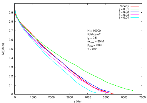
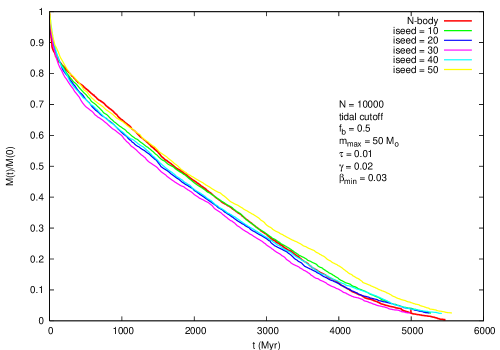
Figure 1: Evolution of the total mass for $N$-body and Monte Carlo models. Left panel for different $\gamma$, right panel for different iseed - initial random number sequence. Parameters of the models are described in the figures.

The best value of $\gamma$ inferred from simulations with $N=2500$ and $10000$ is equal to $0.02$ (see Figure 1 left panel). The $\tau$ and $\beta_{min}$ are equal to $0.01$ and $0.03$, respectively. As can be seen from Figure 1 (right panel) the spread between models (statistical fluctuations) with exactly the same parameters, but with different initial random number sequence (iseed) is very substantial. The spread between results with different $\beta_{min}$ and $\tau$ is well inside the spread connected with different iseed. The statistical fluctuation of the models is larger for smaller $N$ as one can expect.

2.2 Models with full tidal field

The process of escape from a cluster for a steady tidal field is extremely complicated. Some stars which fulfil the energy criterion (binding energy of a star is greater than critical energy $E_{tid_{f}}=-1.5(GM/r_{tid})$) can be still trapped inside a potential wall. Those stars can be scattered back to lower energy before they escape from the system. According to the theory presented by Baumgardt (2001) the energy excess of those stars is decreasing with the increasing number of stars. So the cluster lifetime does not scale linearly with relaxation time as expected from the standard theory. To account for this process in the Monte Carlo code an additional free parameter, $a$, was introduced. The critical energy for escaping stars was approximated by: $E_{tid_{f}}=-\alpha(GM/r_{tid})$, where $\alpha=1.5-a(ln(\gamma N)/N)^{1/4}$. So the effective tidal radius for Monte Carlo simulations is $r_{t_{eff}}=r_{tid}/\alpha$ and it is smaller than $r_{tid}$. This means that for Monte Carlo simulations a system is slightly too concentrated comparable to $N$-body simulations, but the evolution of the total mass is reasonably well reproduced.

Figure 2 shows the evolution of the total mass and the number of binaries for different $\alpha$ for $N=10000$.

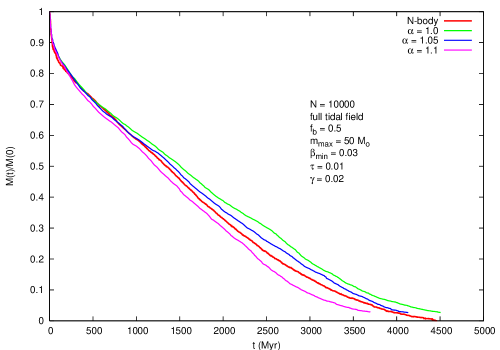
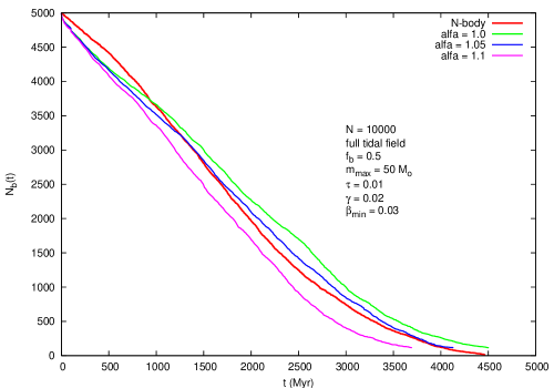
Figure 2: Left panel: evolution of the total mass for $N$-body and Monte Carlo models for different $\alpha$. Right panel: evolution of the number of binaries for $N$-body and Monte Carlo models for different $\alpha$. Parameters of the models are described in the figures.

The value of $\alpha$ inferred from the comparison between $N$-body and Monte Carlo simulations for $N=10000$ is equal to about $1.05$. The other free parameters for the case of full tidal field are the same as for the tidal cutoff case: $\gamma=0.02$, $\tau=0.01$ and $\beta_{min}=0.03$. Again the spread between models with different $\beta_{min}$ and $\tau$ is well inside the spread connected with different iseed. The statistical spread also does not substantially influence the determination of $\alpha$. As can be seen on Figure 2. (right panel) the Monte Carlo code can reproduce well $N$-body simulations not only from respect of the global parameters of the system, but also from respect of the properties connected with binary activities. Despite the fact that the total number of binaries in the system agrees reasonably well with $N$-body simulations the total binding energy of the binaries increases too fast for the Monte Carlo simulations. This is connected with the fact that the present Monte Carlo code does not directly follow the 3- and 4-body interactions as the $N$-body code does, but uses cross sections. The coalescence of binaries induced by dynamical interactions and the exchange interactions are missing in the present Monte Carlo simulations.

2.3 Model of M67

The data from $N$-body simulations of M67 (Hurley et al.  2005) was used in addition to $N=2500$ and $10000$ to finally calibrate the Monte Carlo code, namely $a$. The inferred formula is $\alpha=1.5-3.0(ln(\gamma N)/N)^{1/4}$. The comparison of results from $N$-body and Monte Carlo simulations for M67 confirmed the values of $\gamma$, $\tau$ and $\beta_{min}$ found for smaller $N$ systems. The results of comparison are summarized in Table 1.

Table 1: Monte Carlo and $N$-body results for M67 at 4 Gyr

	$N$-body	MC
$M/M_{\odot}$	2037	1984
$f_{b}$	0.60	0.59
$r_{t}$ $pc^{-1}$	15.2	15.1
$r_{h}$ $pc^{-1}$	3.8	3.03
$M_{L}/M_{\odot}$	1488	1219
$M_{L10}/M_{\odot}$	1342	1205
$r_{h,L10}$ $pc^{-1}$	2.7	2.67
L – stars with mass above $0.5M_{\odot}$ and burning nuclear fuel
L10 - the same as L but for stars contained within 10 pc

Taking into account the intrinsic statistical fluctuations of both methods the results presented in the Table 1 show a reasonably good agreement. At the time of 4 Gyr when the comparison was done, both models consists of only a small fraction of the initial number of stars (about 10%) making the fluctuations even stronger. The Monte Carlo model is slightly too concentrated compared to the $N$-body one. This can be attributed to the parameter $\alpha$, which leads to smaller effective tidal radius than the tidal radius inferred from $N$-body simulations. As can be seen from Figure 3 the Monte Carlo code also reproduces well the results of $N$-body simulations regarding the surface brightness profile and luminosity function.

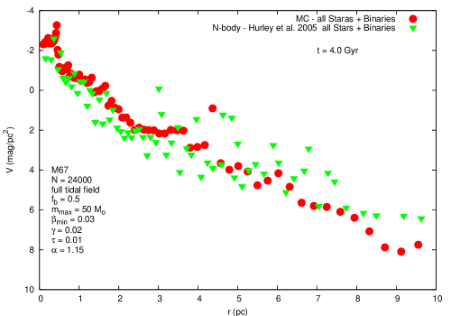
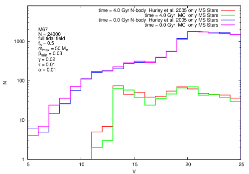
Figure 3: Left panel: surface brightness profile for $N$-body and Monte Carlo models. Right panel: luminosity function for time equal to 0 and 4 Gyr for $N$-body and Monte Carlo models. Parameters of the models are described in the figures.

To finally validate the Monte Carlo model of the old open cluster M67 a brief and very preliminary comparison with the observational data (Montgomery et al.  1993 and Bonatto & Bica 2005) was performed (Figure 4).

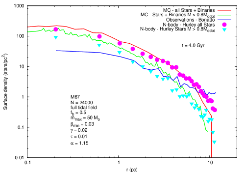
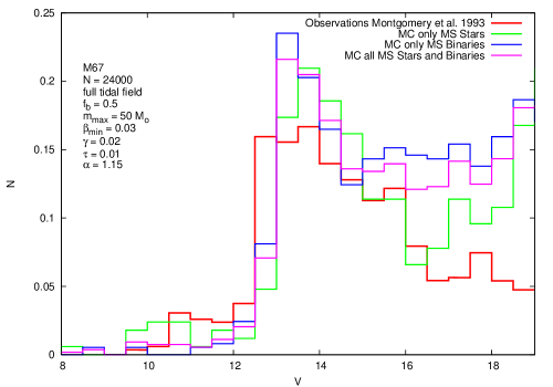
Figure 4: Left panel: surface density profile for Monte Carlo and $N$-body models and for observations (Bonatto & Bica 2005). Right panel: luminosity function for the Monte Carlo model for time = 4 Gyr and for observations (Montgomery et al.  1993) for main sequence stars only, binaries only and both main sequence stars and binaries. Parameters of the models are described in the figures.

Both models: $N$-body and Monte Carlo do not reproduce the observations well. They are too centrally concentrated. Also for the Monte Carlo model the luminosity function is too shallow for dim stars and too high for stars around $V=13\ mag$. In order to achieve a better agreement with observation the initial parameters adopted by Hurley et al.  (2005) have to be slightly changed. Definitely, more work, simulations and observations are needed.

3 Conclusions

It was shown that the Monte Carlo code can be successfully calibrated against small $N$-body simulations. Calibration was done by choosing the free parameters describing the relaxation process, such as: coefficient in the Coulomb logarithm $\gamma=0.02$, minimum deflection angle $\beta_{min}$, time step $\tau$, and coefficient in the formula for the critical energy of escaping stars, $\alpha=1.5-3.0(ln(\gamma N)/N)^{1/4}$. The calibrated code successfully reproduced the $N$-body simulations of the old open cluster M67 (Hurley et al. 2005), which was the main objective of the calibration procedure. The code is able to provide as detailed data as the observations do. However, it showed also some weaknesses, e.g. some important channels of blue stragglers formation are not present (coalescence of binaries due to their dynamical interactions) and too crude treatment of the escape process. The work is in progress to cure these problems (e.g. a few body direct integrations). It was shown also that the Monte Carlo code can be used to model evolution of real star clusters and successfully compare results with observations (see Heggie 2008, in this volume). The very high speed of the code makes it an ideal tool for getting information about the initial parameters of star clusters. It is worth to mention that to complete the model of the M67 cluster only about seven minutes are needed!