A new wavelet-based approach for the automated treatment of large sets of lunar occultation data

Abstract

Context. The introduction of infrared arrays for lunar occultations (LO) work and the improvement of predictions based on new deep IR catalogues have resulted in a large increase in sensitivity and in the number of observable occultations.

Aims. We provide the means for an automated reduction of large sets of LO data. This frees the user from the tedious task of estimating first-guess parameters for the fit of each LO lightcurve. At the end of the process, ready-made plots and statistics enable the user to identify sources that appear to be resolved or binary, and to initiate their detailed interactive analysis.

Methods. The pipeline is tailored to array data, including the extraction of the lightcurves from FITS cubes. Because of its robustness and efficiency, the wavelet transform has been chosen to compute the initial guess of the parameters of the lightcurve fit.

Results. We illustrate and discuss our automatic reduction pipeline by analyzing a large volume of novel occultation data recorded at Calar Alto Observatory. The automated pipeline package is available from the authors.

1 Introduction

For decades, lunar occultations (LO) have occupied a special niche as a technique for high-angular resolution with excellent performance, but relatively inefficient yield. The diffraction fringes that are created by the lunar limb as it occults a background source, provide a unique opportunity to achieve milliarcsecond angular resolution with single telescopes also of relatively small diameter. In terms of instrumentation, LO have always been simple, requiring only a fast photometer. Of course, they have the significant drawback that only sources included in the apparent lunar orbit can be observed (about 10% of the sky), and then only at arbitrary fixed times and with limited opportunities for repeated observations. If one adds that each observation only provides a one-dimensional scan of the source, it is clear that detailed and repeated observations are better performed with long-baseline interferometry (LBI), when available. One should, however, not forget additional important advantages of LO: even for complicated sources, the full, one-dimensional brightness profile can be recovered according to maximum-likelihood principles without any assumptions on the source’s geometry (Richichi 1989A&A…226..366R (1989)). Besides, the limiting sensitivity achieved in the near-IR by LO at the 1.5 m telescope on Calar Alto is K$\approx 8$ mag (Richichi et al. 2006a ). When extrapolated to a 4-meter class telescope or larger, LO appear quite competitive with even the most powerful, LBI facilities (Richichi 1997IAUS..158…71R (1997)).

As a result, although the trend is understandably to develop more flexible, powerful and complex interferometric facilities, there is some balance that makes LO still attractive at least for some applications. It should not be forgotten that the majority of the hundreds of directly-measured stellar angular diameters (Richichi (vlti_2007 (2007)) listed 688, and the numbers keep increasing) were indeed obtained by LO, and that LO are still the major contributor to the discovery of small separation binary stars.

Two recent developments, however, have provided a significant boost to the performance of the LO technique, and have significantly enlarged its range of applications: a) the introduction of IR array detectors that can be read out at fast rates on a small subarray has made it possible to provide a large gain in limiting sensitivity, and b) IR survey catalogues that have led to an exponential increase of the number of sources for which LO can be computed. Literally, thousands of occultations per night could now be potentially observed with a large telescope. We describe in this paper the details and impact of these two factors for LO work. We also address the new needs imposed on data reduction by the potential availability of a large volume of lunar occultation data per night, by describing new approaches to an automated LO data pipeline. We illustrate both the new quality of LO data and their analysis by means of examples drawn from the observation of two recent passages of the Moon over crowded regions in the vicinity of the Galactic Center, carried out with array-equipped instruments at Calar Alto and Paranal observatories.

2 Infrared arrays and new catalogues

A number of reasons make the near-IR domain preferable for LO work with respect to other wavelengths.

First, LO observations are affected by the high background around the Moon which, being mainly reflected solar light, shows an intensity maximum at visible wavelengths. Because of the atmospheric Rayleigh scattering ($\propto\lambda^{-4}$), the background level greatly decreases in the near-IR. At longer wavelengths ($10{\mu}{\rm}m-20{\mu}{\rm m}$), the thermal emission of Earth’s atmosphere and of the lunar surface introduces a high-background level.

Second, the spacing of diffraction fringes at the telescope is proportional to $\lambda^{-\frac{1}{2}}$. Therefore, for two LO observations with the same temporal sampling, one recorded in IR will obtain a higher fringe sampling than one in the visible.

Finally, at least in the field of stellar diameters, there is an advantage to observing in the near-IR because for a given bolometric flux redder stars will present a larger angular diameter.

Being cheap and with a fast time response, near-IR photometers have traditionally represented the detector of choice for LO observations. Richichi (1997IAUS..158…71R (1997)) showed the great increase in sensitivity possible with panoramic arrays, which by reading only the pixels of interest, permit to avoid most of the shot noise generated by the high background in LO. Such arrays are now becoming a viable option, thanks to read-out noises, that are decreasing at each new generation of chips, and to flexible electronics allow us to address a subarray and read it out at millisecond rates. Richichi (1997IAUS..158…71R (1997)) predicted that an 8 m telescope would reach between K=12 and 14 mag, depending on the lunar phase and background, with an integration time of 12 ms at signal–to–noise ratio (SNR)=10. Observations on one of the 8.2 m VLT telescopes, equipped with the ISAAC instrument in the so-called burst mode (Richichi et al. 2006b ), show a limiting magnitude K$\approx$12.5 at SNR=1 and 3ms integration time, in agreement with the decade-old prediction.

These newly-achieved sensitivities call for a corresponding extension in the limiting magnitudes of the catalogues used for LO predictions, and their completeness. In the near-IR, until recently the only survey-type catalogue available was the Two-Micron Sky Survey (TMSS, or IRC, Neugebauer & Leighton 1969tmss.book…..N (1969)) that was incomplete in declination and limited to K$<3$. Already, a 1 m-class telescope equipped with an IR photometer exceeds this sensitivity by several magnitudes (Fors et al. 2004A&A…419..285F (2004), Richichi et al. 1996AJ….112.2786R (1996)). The release of catalogues associated with modern all-sky near-infrared surveys, such as 2MASS (Cutri et al. 2003yCat.2246….0C (2003)) and DENIS (Epchtein et al. 1997Msngr..87…27E (1997)), has helped. Our prediction software ALOP (Richichi AR_thesis (1985)) includes about 50 other catalogues with stellar and extragalactic sources. We have now added a subset of 2MASS with K$\leq 11$, which includes $3.7\times 10^{6}$ sources subject to occultations.

While with the previous catalogues a typical night run close to the maximum lunar phase would cover 100-150 sources over several nights , predictions with 2MASS can include thousands of events observable with a large telescope over one night. Special cases, like the passage of the Moon over crowded, obscured regions in the direction of the Galactic Center, can include thousands of events predicted over just a few hours (Richichi et al. 2006b , Fors et al. 2006a ). Fig. 1 illustrates the two cases. The incompleteness of the catalogues without 2MASS is evident already from the regime $5\leq{\rm K}\leq 7$ mag. At even fainter magnitudes, but still within the limits of the technique as described here, the predictions based on the 2MASS catalogue are more numerous by several orders of magnitude.

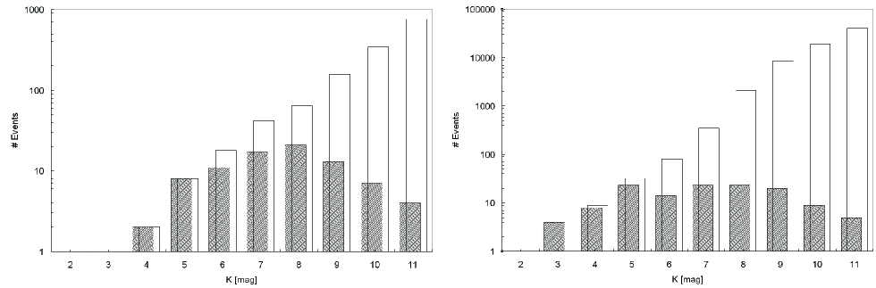
Figure 1: Frequency of lunar occultation events as a function of K magnitude, computed on the basis of all standard catalogues in ALOP (gray bars) and of the 2MASS catalogue only (limited to $K\leq 11$, clear bars). For both cases, we have used the constraints of Moon $\geq 25\degr$ above horizon and Sun $\leq-5\degr$ below horizon. Left: a relatively rich 5-night run, from 7 thru 11 January 2006, at Calar Alto Observatory. Right: part of the night of August 5, 2006 from Paranal, when the Moon reached a minimum approach of $12^{\prime}$ from the Galactic Center. Note the logarithmic scale.

Note that the increase in the number of potential occultation candidates is not reflected automatically in more results. The shift to fainter magnitudes implies that the SNR of the recorded lightcurves is on average lower; LO runs based on 2MASS predictions are now likely to be less efficient in detecting binaries when compared, for example, to studies such as those of Evans et al. (1986AJ…..92.1210E (1986)) and Richichi et al. (2002A&A…382..178R (2002)), especially for large brightness ratios.

3 Automated reduction of large sets of lunar occultation data

In general, LO data are analyzed by fitting model lightcurves. We take as an example the Arcetri Lunar Occultation Reduction software (ALOR), a general model-dependent lightcurve fitting algorithm first developed by one of us (Richichi 1989A&A…226..366R (1989)). Two groups of parameters are simultaneously fitted using a non-linear least squares method. First, those related to the geometry of the event: the occultation time ($t_{0}$), the stellar intensity ($F_{0}$), the intensity of the background ($B_{0}$) and the limb linear velocity with respect to the source ($V_{\rm P}$). Second, those related to physical quantities of the source: for resolved sources; the angular diameter and; for binary (or multiple) stars, the projected separation and the brightness ratio of the components.

In general, the fitting procedure is approached in two steps. First, a preliminar fit assuming an unresolved source model is performed. To ensure convergence, ALOR needs to be provided with reliable initial guesses. We can estimate the geometrical parameters with a visual inspection of the data, and $V_{\rm P}$ is predicted. The source parameters can be refined in a second step. This is done interactively since it requires understanding the nature of each particular lightcurve and the possible correlation between geometrical and physical parameters.

As a result of that great increase in the number of potential occultations, we soon realized that we needed a substantial optimization in the processes of extracting the occultation lightcurves from the raw data and of the interactive evaluation of the LO lightcurves for the estimate of the initial parameter values needed for the fits. We then developed, implemented, and tested a new automatic reduction tool, the Automatic Wavelet-based Lunar Occultation Reduction Package (AWLORP; (Fors 2006b ). This allows both lightcurve extraction and characterization to perform the preliminary analysis of large sets of LO events in a quick and automated fashion. In the following, we describe the main parts of AWLORP, which are schematically illustrated in Fig. 2.

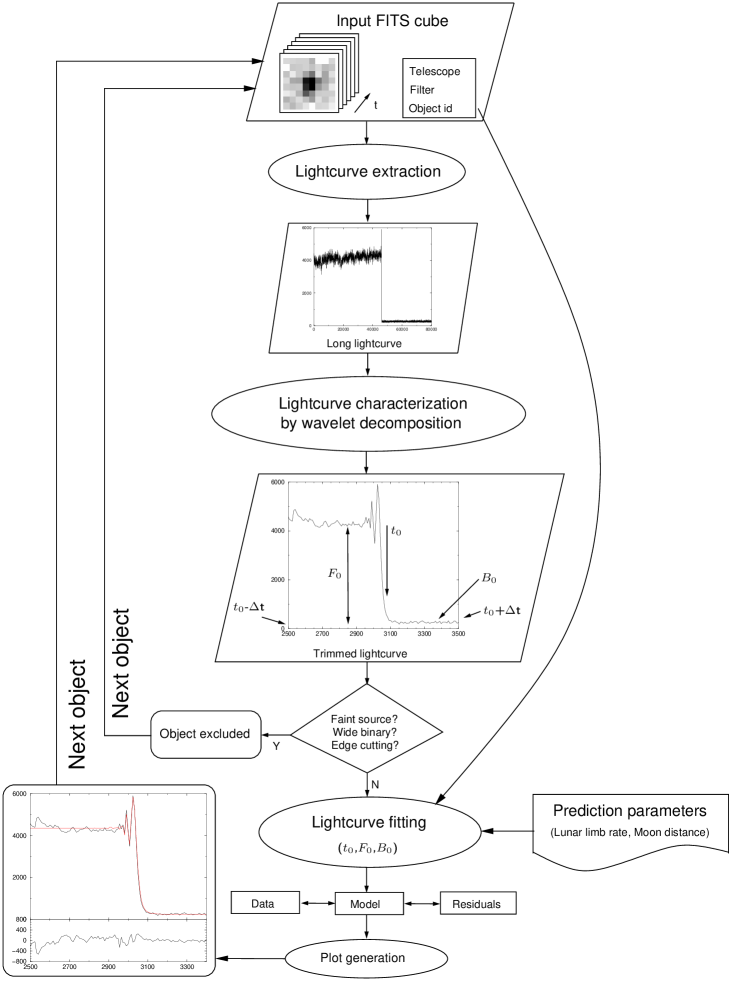
Figure 2: Flow-chart description of AWLORP.

3.1 Input data and lightcurve extraction

In the cases available to us, the LO data are stored in Flexible Image Transport System (FITS) cubes. The number of cube frames is given by the frame exposure and total integration time. Additional information, such as telescope diameter, filter and identificator of the occulted object, are extracted from the FITS cube header and saved in a separate file. In addition, the limb linear velocity and the distance to the Moon as predicted by ALOP are available in a separate file.

An occultation lightcurve must be extracted from the recorded FITS cube file. We explored several methods for this purpose, among them fixed aperture integration, border clipping, Gaussian profile and brightest-faintest pixels extraction. We found these partly unsatisfactory, among other things, because of lack of connectivity across the stellar image and because of sensitivity to flux and image shape variations.

We addressed the problem of connectivity with the use of masking extraction, and two methods were considered. The first method, called 3D-SExtractor, consists of a customization of the object detection package SExtractor (Bertin & Arnouts 1996A&AS..117..393B (1996)) for the case of 3D FITS LO cubes. The algorithm invokes SExtractor for every frame and evaluates its output to decide if the source has been effectively detected. The segmentation map (or source mask) provided by SExtractor defines the object (background) pixels in case of positive (negative) detection. These pixels are used to compute the source (background) intensity before and after the occultation. The second method, called Average mask, consists in performing simple aperture photometry using a predefined source mask. This is obtained by averaging a large number of frames previous to the occultation and by applying a 3$\sigma$ thresholding.

We empirically compared 3D-SExtractor and Average mask methods under a variety of SNR, scintillation, and pixel sampling situations. Although the 3D-SExtractor makes use of a more exact mask definition for every frame, Average mask was found to provide less noisy lightcurves with no evident fringe smoothing. Therefore, we adopted this extraction algorithm as the default in the AWLORP description.

3.2 Lightcurve characterization

Inaccuracies in catalogue coordinates and lunar limb irregularities introduce an uncertainty in the predicted occultation time of about 5 to 10 seconds. To secure the effective registering of an occultation event, the acquisition sequence is started well before the predicted occultation time. This results in a very long extracted lightcurve, typically spanning several tens of seconds. In contrast, the fringes that contain the relevant high-resolution information extend only a few tenths of a second. In addition, to accomplish a proper fitting of this much shorter lightcurve subsample, as mentioned before, we need reliable estimates of $t_{0}$, $B_{0}$ $F_{0}$.

The problem corresponds to detecting a slope with a known-frequency range in a noisy, equally sampled data series. The key idea here is to note that the drop from the first fringe intensity (close to $t_{0}$) is always characterized by a signature of a given spatial frequency. Of course, this frequency depends on the data sampling but, once this is fixed, the aimed algorithm should be able to detect that signature and provide an estimate of $t_{0}$, regardless its SNR. Once $t_{0}$ is known, the other two parameters ($B_{0}$ and $F_{0}$) can be estimated.

This problem calls for a transformation of the data that would be capable of isolating signatures in frequency space, while simultaneously keeping the temporal information untouched. Wavelet transform turns out to be convenient for this purpose.

3.2.1 Wavelet transform overview

The wavelet transform of a distribution $f(t)$ can be expressed as:

$$W(f(t))(a,b)=|a|^{-{1\over 2}}\int_{-\infty}^{+\infty}f(t)\,\psi\biggl{(}{t-b\over a}\biggr{)}\;dt\;,$$ (1)

where $a$ and $b$ are scaling and translational parameters respectively. Each base (or scaling) function $\psi({t-b\over a})$ is a scaled and translated version of a function $\psi$ called mother wavelet, satisfying the relation $\int\psi({t-b\over a})=0$.

We followed the à trous algorithm (Starck & Murtagh 1994A&A…288..342S (1994)) to obtain the discrete wavelet decomposition of $f(t)$ into a sequence of approximations:

$$F_{1}(f(t))=f_{1}(t),\;\;F_{2}(f_{1}(t))=f_{2}(t),\cdots\;.$$ (2)

$f_{i}(t)\;(i=1,\cdots,n)$ are computed by performing successive convolutions with a filter derived from the scaling function, which in this case is a $B_{3}$ cubic spline. The use of a $B_{3}$ cubic spline leads to a convolution with a mask of 5 elements, scaled as (1,4,6,4,1).

The differences between two consecutive approximations $f_{i-1}(t)$ and $f_{i}(t)$ are the wavelet (or detail) planes, $w_{i}(t)$. Letting $f_{0}(t)=f(t)$, we can reconstruct the original signal from the expression:

$$f(t)=\sum_{i=1}^{n}w_{i}(t)+f_{r}(t)\;\;,$$ (3)

where $f_{r}(t)$ is a residual signal that contains the global energy of $f(t)$. Note that $n=r$, but we explicitly substitute $n$ with $r$ to clearly express the concept of $residual$. Each wavelet plane can be understood as a localized frequential representation at a given scale according to the wavelet base function used in the decomposition.

In our case, we are using a multiresolution decomposition scheme, which means the original signal $f(t)$ has twice the resolution of $f_{1}(t)$. This latter has twice the resolution of $f_{2}(t)$, and so on.

3.2.2 Algorithm description

We developed a program to perform a discrete decomposition of the lightcurve into $n_{\rm wav}$ wavelet planes. Note that the choice of $n_{\rm wav}$ depends exclusively on the data sampling and will be discussed later. For example, $n_{\rm wav}=7$ was empirically found to be a suitable value for representing all the features in the frequency space of the lightcurve when the sampling was $8.4$ ms. The 2nd to 7th wavelet planes resulting from the decomposition of the lightcurve of the bright star SAO~190556 (SNR=43) are represented in Fig. 3. The 1st plane was excluded as it nearly exclusively contains noise features not relevant for this discussion. For the sake of simplicity, we will consider this particular lightcurve and sampling value in the description that follows.

We designed an algorithm which estimates $t_{0}$, $B_{0}$ and $F_{0}$ from the previous wavelet planes. This consists of the following two steps: First, it was empirically determined that the 7th plane serves as an invariant indicator of the occultation time ($t_{0}$). In particular, $t_{0}$ coincides approximately with the zero located between the absolute minimum ($t_{0}^{min}$) and maximum ($t_{0}^{max}$) of that plane (see upper right panel in Fig. 3 for a zoomed display of the 7th plane). The good localization of $t_{0}$ in this plane is justified because the first fringe magnitude drop is mostly represented at this wavelet scale. In addition, the presence of noise is greatly diminished in this plane. This is because noise sources (electronics or scintillation) contribute at higher frequencies, and therefore are better represented at lower wavelet scales (planes). In other words, this criteria for estimating $t_{0}$ is likely to be insensitive to noise, even for the lowest SNR cases.

Second, once a first estimate of $t_{0}$ was obtained, $B_{0}$ and $F_{0}$ could be derived by considering the 5th wavelet plane. We found that this plane indicates those values with fairly good approximation. The procedure is illustrated in Fig. 3 and is described as follows:

Figure 3: Schematic of the wavelet-based algorithm for the estimation of $t_{0}$, $F_{0}$, and $B_{0}$ to be used in AWLORP. The lightcurve corresponds to an occultation of SAO~190556 observed at the Calar Alto Observatory, sampled every $8.4$ ms. Left: box with 2nd to 7th wavelet planes resulting from the wavelet decomposition of the original lightcurve. Upper right: the 7th plane is found to be a good indicator of $t_{0}$. A zoomed display of the region around $t_{0}$ is shown. Lower right: a box display of 5th plane (bottom part of this panel) provides the abscissae $t_{\rm b},t_{\rm a}$ to compute $F_{0}$ and $B_{0}$ in the original lightcurve (upper part of the same panel).

1. We consider the abscissa in the 5th plane, corresponding to $t_{0}$ found in the 7th plane.

2. From $t_{0}$, we search for the nearby zeroes in the 5th plane, before and after the above abscissa. We call them $t_{\rm b}$ and $t_{\rm a}$.

3. We estimate $B_{0}$ by averaging the lightcurve values around $t_{\rm a}$ within a specified time range. We empirically fixed this to $\left[-8,8\right]$ samples because it provided a good compromise between improving noise attenuation and suffering from occasional background slopes.

4. The same window average is computed around $t_{\rm b}$. The obtained value ($I_{\rm p}$) represents a mean value of the intensity at the plateau region before the onset of diffraction fringes. Note that the 5th wavelet plane was chosen because its zero at $t_{\rm b}$ is safely before the fringes region in the lightcurve, where the intensity is not constant and, thus, not appropriate for $I_{\rm p}$ calculation.

5. $F_{0}$ is computed by subtracting $B_{0}$ to $I_{\rm p}$.

As in the case of the 7th plane, the contribution in the 5th plane is dominated by signal features represented at this scale, while noise, even the scintillation component, has a minor presence. Therefore, again, the estimation criteria for $B_{0}$ and $F_{0}$ is likely to be well behaved and robust in presence of high noise.

Although AWLORP was demonstrated on a particular data set, its applicability is totally extensible to any sampling of the lightcurve and also to reappearances. To show this, we repeated the previous algorithm description for 6 sets of 100 simulated lightcurves of different samplings (1,2,4,6,8 and 10 ms). For these six samplings, $n_{\rm wav}$ was found to be 8,7,6,6,5 and 5, respectively. Note these values are proportional to a geometric sequence of ratio 2 and argument $(8-n_{\rm wav})$, which is in agreement with the dyadic nature of the wavelet transform we adopted.

3.3 Lightcurve fitting

The algorithm just described has been integrated in an automated pipeline. As shown in the scheme of Fig. 2, the characterization of the lightcurve is used to decide if a fit can be performed succesfully with ALOR. The cases of very faint sources, wide binaries and those lightcurves with some data truncation (i.e. very short time span on either side of the diffraction fringes) are the typical exclusions, and are discussed in Sect. 4.3. In case of positive evaluation, ALOR is executed using the detected values of $t_{0}$,$F_{0}$, and $B_{0}$ as initial guesses. After the preliminary fit is performed, a quicklook plot of lightcurve data, model, and residual files is generated. This process is iterated for all the observed sources.

This automatic pipeline frees us from the most tedious and error-prone part of ALOR reduction. The pipeline spends a few seconds per occultation to complete the whole process described in Fig. 2. For comparison, an experienced user takes 10-20 minutes per event for reaching the same stage of the reduction pipeline. In cases when the data sets included hundreds of occultation events, this difference is substantial. The pipeline was coded entirely in Perl programming language, which turns our to be a powerful and flexible tool for concatenating the I/O streams of independent programs.

Once AWLORP has automatically generated all the single source fit plots, the user can perform a quick visual inspection. The objective of this first evaluation is to separate the unresolved, relatively uninteresting events from those that bear the typical marks of a resolved angular diameter, of an extended component or of a multiple source. These latter will still need an interactive data reduction with ALOR, but they will represent typically only a small fraction of the whole data set.

4 Performance evaluation

We have verified the performance of AWLORP by analysing both simulated and real LO data sets.

4.1 Simulated data

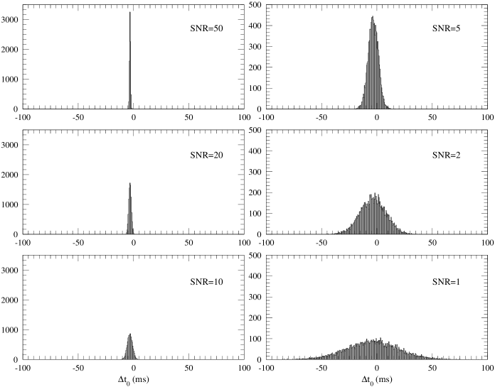
Figure 4: Application of AWLORP to six sets of 10000 simulated lightcurves at 2ms sampling and of different SNRs values. As explained in the text, the offset between the simulated occultation time and the time detected by AWLORP (${\Delta}t_{0}$) is Gaussian distributed with FWHMs inversely proportional to the SNR value, and the histogram peaks are sistematically shifted within the range ${\Delta}t_{0}\sim\left[-4,-2\right]$ms (only 1 to 2 sampling points).

Thanks to a specific module included in ALOR, a set of simulated LO lightcurves was generated for varying SNR values. The noise model assumes three independent noises sources: detector electronics, photon shot-noise, and scintillation, which are of Gaussian, Poisson, and multiplicative nature, respectively (Richichi 1989A&A…226..366R (1989)). With a realistic combination of these three noise sources, we generated six series with SNR $50,20,10,5,2$ and $1$, each of them consisting of 10000 lightcurves. We chose the sampling to be 2ms, which is a realistic value considering what is offered by current detectors.

AWLORP was executed for all the 60000 simulated events. For each lightcurve, we found an estimate of the triplet ($t_{0}$,$F_{0}$,$B_{0}$). The AWLORP only failed to characterize the lightcurve in 10 cases of the noisiest series for which the ALOR fits could not converge. For the remaining 59990 cases, we computed the difference (${\Delta}t_{0}$) between the detected and the simulated occultation time and plotted these differences as shown in Fig. 4. Two comments can be made.

First, the ${\Delta}t_{0}$ distribution is, to a good approximation, Gaussian-shaped. This is in agreement with the fact that the first fringe signature is primarily dominated by Gaussian noise at the wavelet plane ($n_{wav}=7$) employed to estimate $t_{0}$. This noise distribution has its origins in the detector read-out for the faint end (low SNR) and in the shot-noise for the bright end (high SNR), which can be approximated by a Gaussian distribution in this regime. In addition, the typical width of the ${\Delta}t_{0}$ distribution is inversely proportional to the SNR value. A gaussian function was fitted to every histogram, and we found the values $\sigma=23.0,11.7,4.6,2.3,1.1,0.5$ for the cases with SNR$=1,2,5,10,20,50$.

Second, note that the histograms in Fig. 4 are not exactly centered at ${\Delta}t_{0}=0$, but systematically shifted $4$ms to $2$ms (only $2$ to $1$ sampling points). This error is about the Nyquist cut-off frequency of our data sampling. It can be assumed as a limitation imposed by the data and not as an intrinsic constraint of AWLORP. The difference could be corrected by subtracting this small offset to all analyzed lightcurves, but it is in any case of no consequence for the purpose of the subsequent interactive analysis.

4.2 Real data

We considered a set of six real lightcurves. These were recorded in the course of Calar Alto Lunar Occultation Program (CALOP) (Richichi et al. 2006a , Fors et al. 2004A&A…419..285F (2004)). They correspond to a series of SNR values similar to the one discussed in Sect. 4.1.

Figure 5: Application of AWLORP to 6 lightcurves with different SNRs (from top to bottom: 47.2, 22.3, 10.9, 5.9, 2.1 and 1.2) observed as part of the CALOP program. The left side panels show the whole lightcurves (60 seconds). The right side panels show the trimmed lightcurves (spanning only 2 seconds) around the $t_{0}^{d}$ value detected by AWLORP. The occultation time fitted by ALOR using $t_{0}^{d}$ as initial value, $t_{0}^{f}$, are also displayed. Note that even in the faintest SNR case, the occultation time is correctly detected.

The robustness of $t_{0}$ estimation is shown in Fig. 5, where even in the lightcurves at the limit of detection (SNR$=1.2,2.1$) the value of $t_{0}$ is correctly detected. This is confirmed by visual inspection and by an comparison with the predicted values.

To verify this concordance, we ran ALOR fits for all six lightcurves with the AWLORP-detected triplets ($t_{0}$,$F_{0}$,$B_{0}$) as initial values. Even in the faintest cases, ALOR converged for all parameters of the lightcurve model. With regard as $t_{0}$, the difference between the initial and the fitted values never exceeded $13.6$ ms ($1.6$ sample points) as can be seen in Fig. 5.

4.3 Problematic cases

The pipeline just described works well for about 98% of the recorded events. There are, however, a few special situations where the algorithm of Fig. 2 fails. Those can be classified in three distinctive groups:

1. The current version of wavelet-based lightcurve characterization does not support wide binary events. In other words, the pipeline cannot simultaneously determine the values ($t_{0}^{A}$, $B_{0}^{A}$ and $F_{0}^{A}$) and ($t_{0}^{B}$, $B_{0}^{B}$ and $F_{0}^{B}$) for two components $A$ and $B$ separated by more than a hundred of milliarcseconds. Since these cases represent at most a few percent of the overall volume of LO events and they are also relatively uninteresting, this feature has not been implemented yet.

2. Due to observational constraints, to an unusually large prediction error or simply by mistake, sometimes the recording of an event is started too close to the actual occultation time. Since the scaling function has a given size at each wavelet scale, there is a filter ramp that extends over an initial span of data depending on the wavelet plane. For example, in the case of data in Sect. 5 this happens up to 4000 milliseconds from the beginning of the lightcurves, since this is the size of the scaling function at the scale of the 7th plane for the given temporal sampling.

3. Depending on the subarray size employed, the image scale, the seeing conditions or telescope tracking, part of the stellar image might be displaced outside the subarray so that the extracted flux decreases and the shape of lightcurve is affected. Under these circumstances, AWLORP is likely to produce false $t_{0}$ detections. Again, the small number of cases affected does not justify the substantial effort required to improve the AWLORP treatment.

5 Summary

The observation of lunar occultation (LO) events with modern infrared array detectors at large telescopes, combined with the use of infrared survey catalogues for the predictions, has shown that even a few hours of observation can result in many tens if not hundreds of recorded occultation lightcurves. The work to bring these data sets to a stage where an experienced observer can concentrate on accurate interactive data analysis for the most interesting events is long and tedious.

We have designed, implemented, and tested an automated data pipeline that takes care of extracting the lightcurves from the original array data (FITS cubes in our case); of restricting the range from the original tens of seconds to the few seconds of interest near the occultation event; of estimating the initial guesses for a model-dependent fit; of performing the fit; and finally of producing compact plots for easy visual inspection. This effectively reduces the time needed for the initial preprocessing from several days to a few hours, and frees the user from a rather tedious and error-prone task. The pipeline is based on an algorithm for automated extraction of the lightcurves, and on a wavelet-based algorithm for the estimation of the initial parameter guesses.

The pipeline has been tested on a large number of simulated lightcurves spanning a wide range of realistic signal-to-noise ratios. The result has been completely satisfactory: in all cases in which the algorithm converged, the derived lightcurve characterization was correct and consistent with the simulated values. Convergence could not be reached due to poor signal-to-noise ratio in only in ten cases out of 60000. These cases would, of course, be challenging for an interactive data analysis by an experienced observer as well. We also tested the pipeline on a set of real data, with similar conclusions. We identified and discussed the cases that may prove problematic for our scheme of automated preprocessing.

- (1) Bertin, E., & Arnouts, S. 1996, A&AS, 117, 393
- (2) Cutri, R. M., Skrutskie, M. F., van Dyk, S. et al. 2003, The IRSA 2MASS All-Sky Point Source Catalog, NASA/IPAC Infrared Science Archive
- (3) Epchtein, N., et al. 1997, The Messenger, 87, 27
- (4) Evans, D. S., McWilliam, A., Sandmann, W. H., & Frueh, M. 1986, AJ, 92, 1210
- (5) Fors, O., Richichi, A., Núñez, J., Prades, A. 2004, A&A, 419, 285
- (6) Fors O., Richichi, A., Mason, E., Stegmeier, J., Chandrasekhar, T. 2006, Highlights of Spanish Astrophysics IV, Figueras et al. (Eds.), Springer 2007
- (7) Fors, O. 2006, Ph.D. Thesis, Departament d’Astronomia i Meteorologia, Universitat de Barcelona
- (8) Heckmann, O. 1975, Hamburg-Bergedorf: Hamburger Sternwarte, 1975, edited by Dieckvoss, W.
- (9) Neugebauer, G., & Leighton, R. B. 1969, NASA SP, Washington: NASA, 1969
- (10) Richichi, A. 1985, Thesis, Faculty of Physics, Florence University (in italian)
- (11) Richichi, A. 1989, A&A, 226, 366
- (12) Richichi, A., Baffa, C., Calamai, G., Lisi, F. 1996, AJ, 112, 2786
- (13) Richichi, A. 1997, IAU Symp. 158: Very High Angular Resolution Imaging, 158, 71
- (14) Richichi, A., Calamai, G., & Stecklum, B. 2002, A&A, 382, 178
- (15) Richichi, A., & Percheron, I. 2002, A&A, 386, 492
- (16) Richichi, A., Fors, O., Merino, M. et al. 2006, A&A, 445, 1081
- (17) Richichi, A., Fors, O., Mason, E., Stegmeier, J. 2006, The Messenger, 126, 24
- (18) Richichi, A. 2007, ESO Workshop The power of optical/IR interferometry: recent scientific results and 2nd generation VLTI instrumentationi, Richichi, A., Delplancke, F., Paresce, F., Chelli, A. (eds.), Springer 2007, p.31.
- (19) Starck, J.-L., & Murtagh, F. 1994, A&A, 288, 342