Radiography of the Earth’s Core and Mantle with Atmospheric Neutrinos

Abstract

A measurement of the absorption of neutrinos with energies in excess of 10 TeV when traversing the Earth is capable of revealing its density distribution. Unfortunately, the existence of beams with sufficient luminosity for the task has been ruled out by the AMANDA South Pole neutrino telescope. In this letter we point out that, with the advent of second-generation kilometer-scale neutrino detectors, the idea of studying the internal structure of the Earth may be revived using atmospheric neutrinos instead.

The density profile and the shape of the Earth’s core and mantle and their boundary (CMB) determine its geodynamo as well as the feeding mechanism of hotspots at the surface Loper . Knowledge of the CMB is derived from body-wave and free oscillation studies. The information, while more precise than what we can realistically expect from neutrino radiography in the near future, cannot reduce ambiguities in our present model of the CMB associated with the fact that arrays of seismometers only provide regional information, and that free-oscillation data only reveal one dimensional structure. The trade off among density, temperature, and chemical structure for body wave studies increases the uncertainty of the value for the density. For these reasons aspects of the global structure of the CMB region require confirmation. The study presented in this paper indicates that present neutrino detectors have to be operated for 10 years to locate the CMB. IceCube will establish the averaged core and mantle density as a function of longitude thus providing the first independent global survey of the CMB region. We anticipate however that more precise global information on the CMB region will be obtained by longer observation periods or by future large scale neutrino detectors. Early studies of the possibility of doing neutrino tomography date back more than 25 years tomo1-7 . These proposed studying the passage of cosmic beams of high energy (HE) neutrinos through the Earth to diagnose its density. Alternatively, it was suggested to use accelerator beams charpak and to study the propagation effects through matter of oscillating neutrinos; for a review see Ref. winter .

The idea of neutrino tomography is straightforward: the Earth becomes opaque to neutrinos whose energy exceeds $\sim 10$ TeV. The diameter of the Earth represents one absorption length for a neutrino with an energy $\sim$ 25 TeV. Such neutrinos are produced in collisions of cosmic rays with nuclei in the Earth’s atmosphere but, because of the steeply falling energy spectrum of $\sim E_{\nu}^{-3.7}$ of the atmospheric neutrino flux, such events are rare. The hope was that beams of cosmic neutrinos, likely to be associated with the sources of the cosmic rays which reach energies of $10^{8}$ TeV, would provide a plentiful source of neutrinos in the appropriate energy range. These would be detected by HE neutrino telescopes under development at the time. The cosmic beams would perform radiography of the Earth’s interior as it moves relative to the comic source. In light of the recent development of successful and affordable technologies to build very large neutrino telescopes, we revisit the proposal halzini .

Neutrino telescopes detect the Cherenkov radiation from secondary particles produced in the interactions of HE neutrinos in deep water or ice. At the higher energies the neutrino cross section grows and secondary muons travel up to tens of kilometers to reach the detector from interactions outside the instrumented volume reviews . The construction of kilometer-scale instruments such as IceCube at the South Pole and the future KM3NeT detector in the Mediterranean, have been made possible by development efforts that resulted in the commissioning of prototypes that are two orders of magnitude smaller, AMANDA and ANTARES antares . Their successful technologies have, in turn, relied on pioneering efforts by the DUMAND dumand and Baikal baikal , as well as the Macro and Super-Kamiokande collaborations reviewslow . IceCube ice3 is under construction and taking data with a partial array of 1320 ten inch photomultipliers positioned between 1500 and 2500 meter, deployed as beads on 22 strings below the geographic South Pole. Its effective area already exceeds that of its predecessor AMANDA by $\sim$ one order of magnitude. The detector will grow by other $14{\sim}18$ strings in 2007-08 to be completed in 2011 with 80 strings.

AMANDA has observed neutrinos with energies as high as ${\sim}100$ TeV, at a rate consistent with the flux of atmospheric neutrinos (ATM-$\nu$’s) extrapolated from lower energy measurements. It thus establishes limits on any additional flux of cosmic neutrinos in the energy range of interest for Earth tomography. These now reach below $E_{\nu}^{2}\,dN/dE_{\nu}<10^{-11}~{}\text{TeV}\,\text{cm}^{-2}\,\text{s}^{-1}\,\text{sr}^{-1}$ for a diffuse flux hill and $E_{\nu}^{2}\,dN/dE_{\nu}<10^{-10}~{}\text{TeV}\,\text{cm}^{-2}\,\text{s}^{-1}\,\text{sr}^{-1}$ point . From these results Standard Model physics is sufficient to establish that the event rates from cosmic beams per year in a future kilometer-scale detector are limited to $\sim 10$ events from any particular source in the sky and less than $\sim 100$ from the aggregate of sources. Needless to say that the statistics is already uncomfortably small for a beam to be exploited for Earth tomography.

Our main observation is that, with the growth of the detectors, the opportunity arises to exploit the ATM-$\nu$’s that represent the background in the search for cosmic sources, as a beam for studying the Earth. The key point is that, the statistics for ATM-$\nu$’s in the $10$ to $100$ TeV energy range, is superior to those expected from any cosmic sources detected in the future within the upper limits already established by AMANDA observations. Viewed from the South Pole, a uniform flux of ATM-$\nu$’s reaches the detector from the northern half of the sky; it will be modified in the 10 TeV energy region by its passage through the Earth. For instance, neutrinos from vertical to $\sim 30$ degrees have penetrated the core of the Earth before detection, whereas the ones detected at larger angles have traversed the mantle only. Establishing direct evidence for the transition from mantle to core will here be used as a benchmark to evaluate the technique.

We will conclude that IceCube can directly observe the core-mantle transition at the $5\sigma$ level in 10 years. This evaluation is based on modeling of the HE ATM-$\nu$’s that is, at present, still subject to uncertainties. We however establish that, under conservative assumptions, the transition can be observed at the $3\sigma$ level or above.

We use the semianalytical calculation of IceCube event rates described in Ref. GHM . In brief, the expected number of $\nu_{\mu}$-induced events (events arising from $\bar{\nu}_{\mu}$ interactions can be evaluated similarly) in an exposure time $T$ is:

$$N^{\nu_{\mu}}_{\text{ev}}=T\int^{1}_{-1}d\cos\theta\,\int_{0}^{\infty}dl^{\prime}_{\text{min}}\,\int^{\infty}_{l^{\prime}_{\text{min}}}dl\,\int_{E_{\mu}^{\text{fin,min}}}^{\infty}dE_{\mu}^{\text{fin}}\\ \int_{E_{\mu}^{\text{fin}}}^{\infty}dE_{\mu}^{0}\,\int_{E_{\mu}^{0}}^{\infty}dE_{\nu}\frac{d^{2}\phi_{\nu_{\mu}}}{dE_{\nu}\,d\cos\theta}(E_{\nu},\cos\theta)\\ \frac{d\sigma^{\mu}_{CC}}{dE_{\mu}^{0}}(E_{\nu},E_{\mu}^{0})\,n_{T}\,F(E_{\mu}^{0},E_{\mu}^{\text{fin}},l)\,A^{0}_{\text{eff}}$$ (1)

where $d^{2}\phi_{\nu_{\mu}}/(dE_{\nu}\,d\cos\theta)$ is the differential $\nu_{\mu}$ flux in the vicinity of the detector after propagation in the Earth; more below. We use as input the neutrino fluxes from Honda honda extrapolated to match the fluxes from Volkova volkova at higher energies. At the relevant energies, prompt $\nu_{\mu}$’s from charm decay are important. We introduce them according to the recombination quark parton model rqpm but consider alternative estimates also.

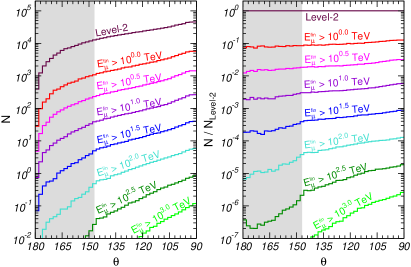
Figure 1: (a) Expected zenith angle distribution of ATM $\nu_{\mu}$ induced events in IceCube for different energy thresholds $E_{\mu}^{\text{fin,min}}$ for the PREM. $\theta$ is the neutrino angle (which at these energies is collinear with the detected muon) as measured from the vertical direction (upgoing-$\nu$ corresponding to $\theta=180$). (b) Ratio of the zenith angle distribution of ATM $\nu_{\mu}$ induced events in IceCube for different energy thresholds $E_{\mu}^{\text{fin,min}}$ over the corresponding one for L2 cuts only. The shadow areas cover the angular size of the Earth core.

$d\sigma^{\mu}_{\text{CC}}/dE_{\mu}^{0}(E_{\nu},E_{\mu}^{0})$ is the differential interaction cross section producing a muon of energy $E_{\mu}^{0}$, After production the muon ranges out in the rock and in the ice surrounding the detector and loses energy to ionization, bremsstrahlung, $e^{+}e^{-}$ pair production and nuclear interactions. This is encoded in $F(E_{\mu}^{0},E_{\mu}^{\text{fin}},l)$ ls which represents the probability that a muon produced with energy $E_{\mu}^{0}$ reaches the detector with energy $E_{\mu}^{\text{fin}}$ after traveling a distance $l$. $n_{T}$ is the number density of nucleons in the matter surrounding the detector.

The details of the detector are encoded in the effective area $A^{0}_{\text{eff}}$ for which we use the parametrization in Ref. GHM describing the response of IceCube after the background rejection quality cuts referred to as “Level-2” (L2) cuts in Ref. ice3 . $l_{\text{min}}=300$ m is the minimum muon track length required for the event to be detected. Effectively $A^{0}_{\text{eff}}$ vanishes for $E_{\mu}^{\text{fin}}\lesssim 100$ GeV.

In order to obtain $d^{2}\phi_{\nu_{\mu}}/(dE_{\nu}\,d\cos\theta)$, one must account for the simultaneous effects of oscillations and inelastic interactions with the Earth matter which lead to the attenuation of the neutrino flux which are different for $\nu_{\tau}$’s and $\nu_{\mu}$’s. hs . This can be achieved by solving a set of coupled evolution equations for the neutrino flux density matrix and for the muon and tau fluxes GHM . In practice, due to the steepness of the ATM-$\nu$ spectra and the small value of the relevant $\Delta m^{2}_{atm}/E_{\nu}$, $d^{2}\phi_{\nu_{\mu}}/(dE_{\nu}\,d\cos\theta)$ can be obtained from:

$$\frac{d^{2}\phi_{\nu_{\mu}}}{dE_{\nu}\,d\cos\theta}(E_{\nu},\theta,L)=\frac{d^{2}\phi_{\nu_{\mu}}^{0}}{dE_{\nu}\,d\cos\theta}(E_{\nu},\theta)\\ P_{\mu\mu}(E_{\nu},L)\,\exp\{-X(\theta)[\sigma_{\text{NC}}(E_{\nu})+\sigma_{\text{CC}}^{\alpha}(E_{\nu})]\}\,,$$ (2)

where $P_{\mu\mu}(E_{\nu},L=2R\left|\cos\theta\right|)$ is the oscillation probability. For $E_{\nu}\gtrsim 1$ TeV, $P_{\mu\mu}\simeq 1$. $X(\theta)$ is the column density of the Earth, and $R$ its radius:

$$X(\theta)=N_{A}\,\int_{0}^{L=2R\left|\cos\theta\right|}\rho_{\text{E}}(\sqrt{R^{2}+z^{2}+2Rz\cos\theta})\,dz\,.$$ (3)

$N_{A}$ is the Avogadro number, and $\rho_{\text{E}}(r)$ is the Earth matter density assumed to be spherically symmetric.

Equation (2) embodies the physics that makes Earth tomography with HE neutrinos possible. At sufficiently high energies, $E_{\nu}\gtrsim 10$ TeV, the attenuation factor $\exp\{-X(\theta)[\sigma_{\text{NC}}(E_{\nu})+\sigma_{\text{CC}}^{\alpha}(E_{\nu})]\}$ becomes relevant. Thus measuring $N^{\nu_{\mu}}_{\text{ev}}$ one can get information on $\rho_{\text{E}}(r)$.

In the left panel of Fig. 1 we show the expected zenith angle distribution of atmospheric $\nu_{\mu}$-induced events in IceCube for different $E_{\mu}^{\text{fin,min}}$ energy threshold as obtained using the Earth matter density profile of the Preliminary Reference Earth Model (PREM) PREM . In the PREM the Earth consists of a mantle extending to radial distance $r\sim 3000$ km below the Earth surface and a core under it with a sharp core-mantle transition in density of about a factor 2. Thus neutrinos arriving with $\theta\gtrsim 147$ degrees ($\cos\theta\lesssim-0.84$) will cross the core in their way to the detector.

In the figure one notices, at sufficiently high energies, a reduction of the number of events for trajectories which cross the core resulting in a “kink” in the angular distribution around $\theta\gtrsim 147$. This feature is more clearly illustrated in the right panel of Fig. 1 where we plot the ratio of the zenith angle distribution of events with energies above $E_{\mu}^{\text{fin,min}}$ divided by the number of events with no additional energy cut, which effectively corresponds to events with a threshold energy $E_{\mu}^{\text{fin,L2}}\sim 100$ GeV.

Figure 1 illustrates the potential of doing Earth tomography with the IceCube ATM-$\nu$ samples. However one must realize that the angular dependence in the ratio shown in the right panel of Fig. 1 is not only due to Earth attenuation factor: there is an additional, Earth-independent, contribution from the variation of the zenith angle distribution of the fluxes with $E_{\nu}$ which does not cancel out in the ratio of events at different energies. In principle this effect could be removed by comparing the ratio of upgoing ($\theta>90$ degrees) and downgoing events ($\theta<90$ degrees). In practice, the overwhelming atmospheric muon background makes the measurement of downgoing $\nu_{\mu}$ events impossible at these energies.

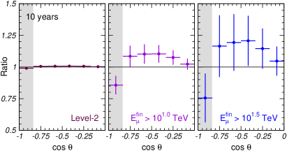
Figure 2: Ratio of zenith angle distribution of expected events for the PREM over the expectations with an homogeneous Earth matter distribution for different values of the energy threshold of the events. The error bars in the figure show the expected statistical error in 10 years of IceCube.

In order to quantify the sensitivity of IceCube to the Earth density profile we study the ratio of observed events above a given energy threshold to the one expected for an Earth of equal mass as ours but with an homogeneous matter distribution, $\rho_{\text{hom}}=3M_{\text{Earth}}/(4\pi R^{3})$:

$$R=\frac{N_{\mu}(E_{\mu}^{\text{fin}}>E_{\mu}^{\text{fin,min}},\,\cos\theta,\,\rho_{\text{PREM}})}{N_{\mu}(E_{\mu}^{\text{fin}}>E_{\mu}^{\text{fin,min}},\,\cos\theta,\,\rho_{\text{hom}})}$$ (4)

In Fig. 2 we show this ratio obtained by integrating the events in the numerator and denominator in 6 angular bins in $\cos\theta$, and for three values of the threshold energy: $E_{\mu}^{\text{fin,L2}}\sim$ 100 GeV, 10 TeV, and 32 TeV. In this plot, trajectories crossing the core are contained in the most vertical bin. In the figure we also show the expected statistical uncertainty $\sigma_{\text{stat},i}$, computed from the expected number of events in each angular bin in the PREM in 10 years of IceCube (see Table 1).

	$E_{\mu}^{\text{fin,min}}$
$[\cos\theta]$	$E_{\mu}^{\text{fin,L2}}$	10 TeV	32 TeV
$[-1.00,-0.83]$	108320	254	27
$[-0.83,-0.67]$	115224	359	49
$[-0.67,-0.50]$	123524	429	62
$[-0.50,-0.33]$	137676	537	82
$[-0.33,-0.17]$	162500	736	111
$[-0.17,0.00]$	205500	1132	169

Table 1: Number of expected atmospheric $\nu_{\mu}$-induced muon events in 10 years of IceCube operation in the different angular bins and energy thresholds for the PREM.

As expected, events with low energy threshold have no sensitivity to the Earth density and consequently the ratio for $E_{\mu}^{\text{fin,L2}}\sim 100$ GeV is practically constant and equal to 1. As $E_{\mu}^{\text{fin,min}}$ increases the ratio becomes increasingly different from 1, reflecting the fact that the effect of the Earth matter profile becomes more evident. The strategy is then obvious. One uses the measured zenith angular distribution of the L2 event sample as normalization to obtain the expectations for a constant density Earth at higher energies, $N_{\mu}(E_{\mu}^{\text{fin}}>E_{\mu}^{\text{fin,min}},\,\cos\theta,\,\rho_{\hom})$. By comparing the expectations with observation, one can quantify the sensitivity to the Earth matter profile.

After normalizing to the observed L2 distribution residual theoretical uncertainties remain associated with the predicted zenith angle distribution. They include systematic effects in calibration, theoretical errors in the energy-angle dependence in the atmospheric fluxes due to the uncertainties in the $K/\pi$ ratio as well as in the contribution from charm (which are expected to be the largest at the relevant energies), and the uncertainties in the neutrino interaction cross sections. Over the limited energy range relevant here, we conservatively account for those by introducing three systematic errors in the analysis: an overall normalization error of 20%, and angular tilt uncertainty of 5% between horizontal and vertical events and an additional $\sigma_{\text{sys},i}=1$% uncertainty due to uncorrelated systematics for each angular bin. With this we construct two simple $\chi^{2}$ functions as

$$\chi^{2}_{\text{nh}} =\mathop{\mathrm{Min}}_{\begin{subarray}{c}\xi_{\text{norm}}\\ \xi_{\text{$\theta$-tilt}}\end{subarray}}\Big{\{}\sum_{i=1}^{5}\frac{[R_{i}-R^{\text{th}}_{i}]^{2}}{\sigma_{\text{stat},i}^{2}+\sigma_{\text{sys},i}^{2}}+\xi_{\text{norm}}^{2}+\xi^{2}_{\text{$\theta$-tilt}}\Big{\}}\,,$$ (5)

$$\chi^{2}_{\text{cm}} =\frac{[R_{\text{c}}-R^{\text{th}}_{\text{c}}]^{2}}{\sigma_{\text{stat,c}}^{2}+\sigma_{\text{sys,c}}^{2}}+\frac{[R_{\text{m}}-R^{\text{th}}_{\text{m}}]^{2}}{\sigma_{\text{stat,m}}^{2}+\sigma_{\text{sys,m}}^{2}}$$ (6)

where $R^{\text{th}}_{i}=(1+0.2\,\xi_{\text{norm}})\,(1+0.05\,\langle\cos\theta\rangle_{i}\,\xi_{\text{$\theta$-tilt}})$ and we have defined $R_{\text{c}}=R_{1}$ and

$$R_{\text{m}}=\frac{\displaystyle\sum_{i=2}^{5}N_{\mu}^{i}(E_{\mu}^{\text{fin}}>E_{\mu}^{\text{fin,min}},\,\rho_{\text{PREM}})}{\displaystyle\sum_{i=2}^{5}N_{\mu}^{i}(E_{\mu}^{\text{fin}}>E_{\mu}^{\text{fin,min}},\rho_{\text{hom}})}\,,$$ (7)

with $\sigma^{2}_{\text{stat,m}}={\displaystyle\sum_{i=2}^{5}}\sigma^{2}_{\text{stat},i}$ and $\sigma^{2}_{\text{sys,m}}=4\times(1\%)^{2}$. In Eq. (6) $R^{\text{th}}_{\text{c}}$ and $R^{\text{th}}_{\text{m}}$ are the corresponding theoretical predictions including the normalization and tilt factors which minimize $\chi^{2}_{\text{nh}}$. In the $\chi^{2}$ functions we have, conservatively, not included the events in the most horizontal bin $\cos\theta>-0.17$ where larger backgrounds from possible remaining misreconstructed downgoing muons may be expected. In choosing the optimum energy threshold for this comparison, one has to take into account that, as the energy increases, the Earth matter profile becomes more evident but the statistics decreases and so does the achievable precision. For these simple observables, a compromise sensitivity is achieved for $E_{\mu}^{\text{fin,min}}=10$ TeV.

$\chi^{2}_{\text{nh}}$ quantifies the rejection power against the hypothesis of a homogeneous Earth density, while $\chi^{2}_{\text{cm}}$ gives the sensitivity to the specific difference in density between the core and the mantle. We find that, if no deviation from the PREM predictions is observed, in 10 years IceCube can reject the homogeneity of the Earth with a $\chi^{2}_{\text{nh}}=11.5$ ($3.4\sigma$) which can reach $\chi^{2}_{\text{nh}}=22$ ($4.7\sigma$) if the theoretical and systematic uncertainties are reduced to be below the statistical errors. Correspondingly, the difference in density between the core and mantle can be established with $\chi^{2}_{\text{cm}}=\text{9--22}$ ($3\sigma$–$4.7\sigma$).

In summary, we conclude that IceCube will be able to measure the averaged core and mantle density with a significance that reaches, conservatively, $3\sigma$ in a decade. Our best guess is that a result can be obtained at the $5\sigma$ level.

Work supported by Grants from U.S. NSF No. OPP-0236449 and PHY-0354776, and U.S. DOE No. DE-FG02-95ER40896, from Spanish MEC, FPA-2004-00996, FPA-2006-01105 and FPA-2007-66665-C02-01 and from Comunidad Autónoma de Madrid P-ESP-00346.

References

- (1) D.E. Loper and T. Lay, J. Geophys. Res. B4, 6397 (1995).
- (2) L. V. Volkova and G. T. Zatsepin, Bull. Russ. Acad. Sci. Phys. 38, 151 (1974); I. P. Nedyalkov, Balatonfuered 1982, Proceedings, Neutrino ’82, Vol. 1, 300-302; T. L. Wilson, Nature 309, 38 (1984); G. A. Askarian, Sov. Phys. Usp. 27 (1984) 896; C. Kuo et al., Earth Plan Sci Lett 133, 95 (1995); A. B. Borisov, B. A. Dolgoshein and A. N. Kalinovsky, Yad. Fiz. 44 (1986) 681; P. Jain, J. P. Ralston and G. M. Frichter, Astropart. Phys. 12, 193 (1999); M. M. Reynoso and O. A. Sampayo, Astropart. Phys. 21, 315 (2004).
- (3) A. De Rujulaet al., Phys. Rept. 99, 341 (1983).
- (4) W. Winter, arXiv:physics/0602049.
- (5) F. Halzen, Eur. Phys. J. C 46, 669 (2006)
- (6) T. K. Gaisser, F. Halzen, and T. Stanev, Phys. Rept. 258, 173 (1995); J.G. Learned and K. Mannheim, Ann. Rev. Nucl. Part. Science 50, 679 (2000); F. Halzen and D. Hooper, Rept. Prog. Phys. 65, 1025 (2002).
- (7) M. Bouwhuis et al., J. Phys. Conf. Ser. 60, 239 (2007).
- (8) J. Babson et al., Phys. Rev. D 42, 3613 (1990).
- (9) V. A. Balkanov et al., Nucl. Phys. Proc. Suppl. 118, 363 (2003).
- (10) T. Kajita, Rept. Prog. Phys. 69, 1607 (2006).
- (11) A. Achterberg et al., Astropart. Phys. 26, 155 (2006); J. Ahrens et al., Astropart. Phys. 20, 507 (2004).
- (12) G. Hill, 30th ICRC, Merida, Mexico, 2007, [1103]
- (13) A. Achterberg et al., Phys. Rev. D 75, 102001 (2007)
- (14) M.C. Gonzalez-Garcia et al., Phys. Rev. D 71, 093010 (2005),
- (15) M. Honda et al., Phys. Rev. D 70, 043008 (2004).
- (16) L. V. Volkova, Sov. J. Nucl. Phys. 31, 784 (1980)
- (17) E. V. Bugaev et al., Phys. Rev. D 58, 054001 (1998)
- (18) P. Lipari and T. Stanev, Phys. Rev. D 44 (1991) 3543.
- (19) F. Halzen and D. Saltzberg, Phys. Rev. Lett. 81, 4305 (1998).
- (20) A.M. Dziewonski and D.L. Anderson, Phys. Earth Planet. Inter. 25, 297 (1981).