On the viability of the shearing box approximation for numerical studies of MHD turbulence in accretion disks

Abstract

Context. Most of our knowledge of the nonlinear development of the magnetorotational instability (MRI) relies on the results of numerical simulations employing the shearing box (SB) approximation. A number of difficulties arising from this approach have recently been pointed out in the literature.

Aims. We thoroughly examine the effects of the assumptions made and numerical techniques employed in SB simulations. This is done to clarify and gain a better understanding of those difficulties, in addition to a number of additional serious problems raised here for the first time, and of their impact on the results.

Methods. We used analytical derivations and estimates as well as comparative analysis to methods used in the numerical study of turbulence. We performed numerical experiments to support some of our claims and conjectures.

Results. The following problems, arising from the (virtually exclusive) use of SB simulations as a tool for the understanding and quantification of the nonlinear MRI development in disks, are analyzed and discussed: (i) inconsistencies in the application of the SB approximation itself; (ii) the limited spatial scale of the SB; (iii) the lack of convergence of most ideal mgnetohydrodynamical (MHD) simulations; (iv) side-effects of the SB symmetry and the non-trivial nature of the linear MRI; and (v) physical artifacts arising from the very small box scale due to periodic boundary conditions.

Conclusions. The computational and theoretical challenge posed by the MHD turbulence problem in accretion disks cannot be met by the SB approximation, as it has been used to date. A new strategy to confront this challenge is proposed, based on techniques widely used in numerical studies of turbulent flows - developing (e.g., with the help of local numerical studies) a sub-grid turbulence model and implementing it in global calculations.

1 Introduction

A physical mechanism for angular momentum transport outward is needed for the theoretical modelling of accretion disks. Prendergast & Burbidge (1968) proposed the existence of thin accretion disks to explain some galactic X-ray sources. They realized that such disks must be characterized by an enhanced viscosity, orders of magnitude larger that the microscopic viscosity expected for the gas comprising the disks. Given the likelihood that such flows are turbulent, they estimated the value of this enhanced viscosity with the help of a mixing-length theory. A few years later, Shakura & Sunayev (1973) and Lynden-Bell & Pringle (1974) successfully bypassed the specific lack of understanding of turbulence (a situation that is largely still with us) by employing physically motivated parametrizations of this turbulent viscosity. In doing so thin accretion disks, for the first time, could be modeled in a variety of astrophysical settings. In turn, this has brought about significant progress in our understanding of these important systems.

Because the value and nature of the now famous nondimensional viscosity parameter $\alpha$ still remains a theoretical unknown, phenomenological approaches are usually employed to determine its value. Such an approach also involves identifying an instability (or combination of instabilities) that is responsible for the emergence of accretion disk turbulence. This quest, according to this strategy, has become the focus of intense (and sometimes contentious) research for the three decades following the above mentioned ground-breaking studies. Notwithstanding the current lack of a general theory of turbulence, the identification of an instability process and, hopefully, also understanding the transition from laminar flow into some turbulent-like steady state (or at least quasi-steady one) has seemed to be the most promising strategy to quantify angular momentum transport and energy generation in accretion disks. However, no definitive candidate hydrodynamical instability had been convincingly identified and widely accepted before Balbus & Hawley (1991) discovered that weak magnetic fields destabilize differential Keplerian rotation. The linear magnetorotational instability (MRI; Velikhov 1959, Chandrasekhar 1960) was shown to operate under conditions characterizing rotationally-supported magnetized cylindrical disks.

This important study has inspired intensive research activity on the linear MRI and its nonlinear development. This mechanism has been investigated for various physical conditions, geometries, and boundary conditions (BC), and it has been approached using a number of mathematical methods. The complexity of its nonlinear development requires employing numerical computational methods. Understanding, or at least numerically simulating in a faithful way, the nonlinear transition and saturation processes (even through the use of some approximations), is indispensable if the aim is to improve the more than 30 years old phenomenological $\alpha$-model.

As the general problem of the development of magnetohydrodynmical (MHD) turbulence in accretion disks is a formidable one, various approximations have been utilized. The purpose of this paper is to assess the viability of one of the approximations most commonly used in numerical studies - the shearing box (SB), also known as the “shearing sheet.” The review articles by Balbus & Hawley (1998) and Balbus (2003) contain a comprehensive summary of the results of linear studies as well as SB numerical ones (under various physical conditions) available at the time of these reviews, together with a thorough list of references, of which only some will be referred to here.

In the recent years, a number of new and improved (in resolution) SB calculations subject to differing conditions and employing different numerical methods have been reported on. Some results of these studies have raised a number of significant issues regarding a central question pertaining to accretion disks: a quantitative estimate and scaling of the angular transport in a saturated MHD turbulent state (e.g, Pessah, Chan & Psaltis 2007; Lesur & Longaretti 2007, Fromang et al. 2007). It is of no surprise that the estimate of this transport, or the ”effective $\alpha$”, which is a quantitative measure thereof, must depend upon those relevant nondimensional numbers characterizing the flow. In particular, these numerical studies indicate that the transport is proportional to some positive power of the magnetic Prandtl number of the flow.

In parallel, a number of related approximate analytical treatments using asymptotic analysis have been published (Knobloch & Julien 2005; Umurhan, Menou & Regev 2007; Umurhan, Regev & Menou 2007, hereafter URM07). The latter two studies found the above-mentioned scalings in some limits of a magnetic Taylor-Couette thin gap configuration (formally different from the SB only in the boundary conditions), while the former work showed that transport diminishes in proportion to the inverse of the Reynolds number and/or the magnetic Reynolds number for the nonlinear development of coupled channel mode (CM) solutions.

Recent years have also seen experimental efforts to observe the MRI and its nonlinear development in the laboratory. These have been done primarily in a magnetic Taylor-Couette (mTC) setup with an applied axial or helical magnetic field. In these studies (see, e.g., Ji, Goodman & Kageyama 2001; Noguchi et al. 2002; Sisan et al. 2004; Hollerbach & Rüdiger 2005; Liu, Goodman & Ji 2006; Stefani et al. 2006; and references therein) MRI turbulence has only been reported for experiments with helical fields, in which the azimuthal field component is significant. Even for this case some controversy remains over the interpretation of the results (Liu et al 2006; Rüdiger & Hollerbach 2007).

Most of the existing SB calculations (at least of the early ones) employed a base state with a constant vertical magnetic field and followed the development of perturbations on this state. This situation, usually referred to as non-zero, or fixed net flux (herafter fixed-flux), seems to be the most appropriate for disks threaded by external magnetic fields (whether primordial or originating from the central accreting object). The majority of existing numerical works of this sort have used ideal (that is, non-dissipative) MHD SB equations with periodic boundary conditions (periodic-BC) in the manner employed, for example, by Hawley et al. (1995), but the very recent calculations of Lesur & Longaretti (2007) include explicit viscosity $\nu$ and resistivity $\eta$ in a small shearing box (SSB, see below), high-resolution, numerical simulation. Systematically changing the Reynolds number (${\rm Re}$) and the magnetic Prandtl number ${\rm P}_{m}\equiv\nu/\eta$, in some range, these authors aimed at uncovering the trends and scalings of relevant physical properties, notably angular momentum transport, with the relevant non-dimensional number(s). A number of studies also exist demonstrating the role of the MRI as an essential ingredient for internal dynamo action in the case where the base state has zero net flux (hereafter zero-flux). It is reasonable to suggest that the zero-flux case should be relevant to disks (or disk regions) that are not threaded by magnetic flux. The most recent zero-flux calculations in the SB framework with relatively high resolution have been reported by Fromang & Papaloizou (2007) and by Fromang et al. (2007) These studies (both employing periodic-BC) focus on the issue of convergence (i.e., numerical resolution) in ideal SB calculations and on the $\rm Re$ and ${\rm P}_{m}$ dependencies of the transport in dissipative conditions.

Recently King, Pringle & Livio (2007), hereafter KPL07, pointed out the discrepancy (of at least one order of magnitude) between the values of $\alpha$ inferred from observations and the estimates of this parameter based on (mainly the early) SB numerical simulations. In particular they reexamined the conclusion, reasoned by Hawley, Gammie & Balbus (1995) based on their fixed-flux SB simulations, that the effective $\alpha$ is dependent (almost linearly) on the value of the imposed $B_{z}$. Similar scaling has also been reported by Sano et al. 2004 and Pessah, Chan & Psaltis 2007, but the latter also found a pre-factor depending on the box size as $L^{0.6}$. They concluded from this puzzling result that fixed-flux simulations are not likely to be adequate for accretion disks and the zero-flux ones should be used instead. They also identified several theoretical difficulties of the SB simulations - limitation of scale, problematic boundary conditions, question of convergence of the simulations (numerical resolution issues), and a possible breakdown of the MHD approximation. Rincon, Ogilvie & Proctor (2007) recently published a significant study, hereafter ROP07, in which they discovered that a self-sustaining nonlinear dynamo process may operate in Keplerian shear flows in the zero-flux case. In this dynamo process, the MRI is not a bona-fide linear instability, resulting from a modal stability analysis of the base flow, but rather participates in one of the stages of the dynamo action. We shall refer to the role of the MRI in this process as mediating rather than “driving”, or “inducing” (which will be the term in the fixed-flux case) MHD turbulence. It is important to note, in the context of the present work, that this analysis was done in the framework of a rotating magnetic plane Couette flow (rmpC), that is, one in which realistic wall boundary conditions (wall-BC) were employed. This is in contrast to the majority of SB calculations wherein periodic-BC are used instead.

Turbulent magnetic dynamo theory, which is concerned with the question of magnetic field generation in cosmic bodies (see, e.g., Moffat 1978; Parker 1979), is a principally similar MHD problem and it has been studied extensively using direct numerical simulations (e.g, Cattaneo & Hughes 1996; Brandenburg & Donner 1997; Schekochihin et al. 2007 and references therein). The issues regarding the computational domain, resolution and BC in such calculations, and their effect on the results and findings have always seriously been considered (see, e.g., Blackman & Field 2000). We mention this theory here at the outset because we will use it as an example of another intensively studied MHD turbulence problem in which progress has been quite impressive.

In this paper, we shall examine in detail the viability of the SB approximation to the study of angular momentum transport (resulting from MHD turbulence related to the MRI) in accretion disks. We shall discuss it for both the fixed-flux case (where the MRI is expected to induce MHD turbulence via a supercritical transition, i.e., it is a linear instability in the usual modal sense) and the zero-flux case (where the MRI is invoked in a self-sustaining process involving a subcritical transition). We shall not only address and expound on some of the issues discussed by KPL07 and others, but also point out and analyze in detail a number of other very significant difficulties. This will lead us to the conclusion that the SB approximation, as used in the great majority of the existing numerical simulations, suffers from limitations that make it inadequate for the qualitative and quantitative understanding of the nonlinear development of the MRI in accretion disks.

Our paper is organized as follows. We start by reviewing a recent fairly exact derivation of the SB approximation distinguishing between the two limits of this approximation: the small shearing box (SSB) and the large shearing box (LSB). In the next section the relevant physical length scales of the problem are discussed and related to the box scale, yielding an answer to the question: which physical properties can be expected to be faithfully uncovered in SSB and in LSB? In Sect. 4 we consider numerical resolution (convergence) in SB simulations and its implications on the numerical results and the conclusions thereof. In Sect. 5, we point out the symmetry properties of the SB equations and of the boundary conditions used in their simulations (which are not globally valid in an accretion disk model) and their effect on the solutions to the linear and nonlinear problems. This is followed in Sect. 6 by a discussion of the SB energetics and the effects of periodic boundary conditions on it, when the box size is not large enough. We also perform a number of numerical experiments to demonstrate this important issue.

As far as investigating the properties of MRI induced and/or mediated MHD turbulence is concerned, we finally discuss which (if any) of the setups - SB, mTC or rmpC - would be an appropriate venue for local numerical studies. In this context, we stress the value of analytical and semi-analytical studies for the purpose of better understanding numerical simulations and experiments. We also suggest possible promising strategies for conducting global (disk scale) studies, exploiting the knowledge gained from the local ones. The ultimate goal in all of this is to find a viable way to quantitatively assess the turbulent angular momentum transport and energy dissipation for the modeling of accretion disks.

2 The Shearing Box (SB) approximation

The essence of the SB approximation is in its local approach, that is, the resulting equations for the perturbations on a steady base flow are approximately valid in a small region (a Cartesian box) around a typical point in the disk. The global MHD base flow in an almost Keplerian accretion disk is not only rotating and strongly sheared, but it is also inhomogeneous, non-isotropic (endowed with non-zero gradients in density and other physical variables and these gradients have very different scales in different directions) and swirling (streamlines are curved).

The SB approximation, with its emphasis on the effect of shear, is not new and has been introduced in an astrophysical context long ago by Goldreich & Lynden Bell (1965) (see also Toomre 1964) in their study of sheared gravitational instabilities in a galaxy. Hawley & Balbus (1991) adapted the approximation to the numerical study of the MRI in accretion disks and it has been routinely used ever since. Umurhan & Regev (2004) followed a systematic derivation of the approximation, using asymptotic scaling arguments with the purpose of quantifying the approximations that are made leading to the SB (see Appendix A of that paper). Even though a purely hydrodynamical case was considered there, the addition of MHD terms is straightforward, because the magnetic field remains invariant in a transformation to a moving frame as long as the velocities involved are non-relativistic (naturally with respect to an observer in the laboratory frame).

We summarize here the procedure for an MHD base flow in a thin Keplerian disk with a constant vertical magnetic field (as a convenient example). This is done to set the stage and also emphasize the difference between the two self-consistent limits of the approximation. The derivation starts by picking a point in the disk, $(r_{0},\phi_{0},z=0)$ in cylindrical coordinates, transforming the relevant full equation set into a frame rotating with the Keplerian angular velocity appropriate for this point $\Omega_{0}\equiv\Omega_{\rm K}(r_{0})$, and looking at the equations in a Cartesian box - a small neighborhood around the point $r_{0}$. Non-dimensionalization of the equations that describe a thin disk brings out two small non-dimensional parameters - $\epsilon$ (the typical disk height $h_{0}$, in units of $r_{0}$) and $\delta$ (the box size in the same units). The next step is the expansion (up to first order in $\delta$) of the dependent variables of the laminar (mean) base flow, Keplerian rotation in this case, in the neighborhood of $r_{0}$, and the removal of the mean flow. This results in a set of partial differential equations for the disturbances that are fluctuations atop a base state (i.e, deviations from a laminar flow profile with constant vertical magnetic field). Identifying the radial (shear-wise) direction with the Cartesian coordinate $x$, the azimuthal (stream-wise) direction with $y$, leaving $z$ as the vertical coordinate and neglecting the curvature terms (consistently with the smallness of $\delta$) finally yields the SB equations. For details see Umurhan & Regev (2004), who identified two limits of the SB approximation, depending on the ordering of the small parameters $\epsilon$ and $\delta$. In the first one, a box whose size is much smaller than the vertical scale height of the disk, i.e., $\delta\ll\epsilon$ is considered, and thus the unperturbed state of linear shear may be considered homogeneous. The perturbations are then incompressible and acoustics are filtered out. This is the SSB. The second limit, LSB, is the case $\delta={\cal O}\left({\epsilon}\right)$, in which vertical stratification as well as compressibility must be taken into account and the situation is considerably more complicated than SSB. We note here in passing that a typical thin accretion disk has $\epsilon\sim 10^{-2}$, and this is thus the LSB ($\delta=\epsilon$) scale in units of $r_{0}$, while the SSB ($\delta=\epsilon^{2}$) scale is in these units $\sim 10^{-4}$.

For the purposes of this paper, it will suffice to consider here the simple SSB for dissipative MHD flow with a fixed vertical background field, possibly zero, and constant density ($=1$ in our units), because the issues we want to deal with do not depend on additional details. The velocity perturbations (deviations from the laminar profile, in units of $\Omega_{0}r_{0}\delta$) are ${\bf u}\equiv(u,v,w)$ and those in the magnetic field (expressed in units of $\tilde{V}_{A}^{2}$, a typical Alfvén speed squared, appropriate for the background field $B_{0}$) are correspondingly ${\bf b}\equiv(b_{x},b_{y},b_{z})$. The total pressure perturbation (in units of $\epsilon^{2}\Omega_{0}^{2}r_{0}^{2}$, see below) is written as $\varpi\equiv p+(2\beta)^{-1}b^{2}$, where $\beta\equiv\epsilon^{2}\Omega_{0}^{2}r_{0}^{2}/\tilde{V}_{A}^{2}$ (the “plasma beta”). Additionally, lengths are scaled by the box size ($\delta r_{0}$) and time by the Keplerian time $(1/\Omega_{0})$. With these assumptions and definitions the non-dimensional SSB equations in the rotating Cartesian frame explained above read,

$$\qquad\nabla\cdot{\bf u}=0,\quad\nabla\cdot{\bf b}=0,$$ (1)

$$(\partial_{t}-q\Omega_{0}x\partial_{y})u - 2\Omega_{0}v+{\bf u}\cdot\nabla u=-\partial_{x}\varpi+$$ (2)

$$+ {1\over\beta}\left(B_{0}\,\partial_{z}+{\bf b}\cdot\nabla\right)b_{x}+{1\over{\rm Re}}\nabla^{2}u,$$

$$(\partial_{t}-q\Omega_{0}x\partial_{y})v + (2-q)\Omega_{0}u+{\bf u}\cdot\nabla v=-\partial_{y}\varpi+$$ (3)

$$+ {1\over\beta}\left(B_{0}\,\partial_{z}+{\bf b}\cdot\nabla\right)b_{y}+{1\over{\rm Re}}\nabla^{2}v,$$

$$(\partial_{t}-q\Omega_{0}x\partial_{y})w + {\bf u}\cdot\nabla w=-\partial_{z}\varpi+$$ (4)

$$+ {1\over\beta}\left(B_{0}\,\partial_{z}+{\bf b}\cdot\nabla\right)b_{z}+{1\over{\rm Re}}\nabla^{2}w,$$

$$(\partial_{t}-q\Omega_{0}x\partial_{y}){\bf b} = B_{0}\partial_{z}{\bf u}+$$ (5)

$$+ q\Omega_{0}b_{x}{\bf\hat{y}}+\nabla\times({\bf u}\times{\bf b})+\frac{1}{{\rm Re}_{m}}\nabla^{2}{\bf b},$$

where the Reynolds number ($\rm Re$) and its magnetic counterpart, ${\rm Re}_{m}\equiv{\rm Re\cdot P}_{m}$, are defined in the SSB as:

$${\rm Re}\equiv\frac{\Omega_{0}r_{0}^{2}\delta^{2}}{\nu},\qquad{\rm Re}_{m}\equiv\frac{\Omega_{0}r_{0}^{2}\delta^{2}}{\eta}.$$

For the sake of some generality and convenience we have kept $\Omega_{0}$ and $B_{0}$ (which are actually equal to 1 in our units) and $q\equiv-(d\ln\Omega/d\ln r)_{0}$ (equal to $3/2$ for a Keplerian rotational law). Note that to the extent to which these equations represent a small disk section, if the base flow deviates significantly from Keplerian rotation, then the horizontal pressure gradient does not drop out of the equations and the system would not be a proper representation of a rotationally-supported disk. In addition, it is perhaps important to explain the choice of the pressure unit. In a disk that is vertically supported by pressure, the vertical scale-height is determined by the sound speed and gravity (that can be expressed in terms of the local Keplerian speed). Thus at a point $r_{0}$, we obtain that this vertical scale is approximately given by $h_{0}=\tilde{v}_{s}/\Omega_{0}$, where $\tilde{v}_{s}$ is the typical sound speed. Therefore $\epsilon=\tilde{v}_{s}/(\Omega_{0}r_{0})$ and it is small if the Keplerian velocity is highly supersonic. As we have pointed out above, on the SSB scale the flow is essentially incompressible and the sound speed loses its meaning. By scaling the pressure with $\epsilon^{2}\Omega_{0}^{2}r_{0}^{2}$, we thus consistently express the vertical size of the disk.

It is possible to reformulate the above SSB equations in terms of shearing coordinates in the same way as implemented by Goldreich & Lynden-Bell (1965). These coordinates are written into a frame that is shearing exactly as the background flow itself on the SB scale (linearly). This coordinate system $(\xi,\eta,\zeta,\tau)$ is thus defined in terms of the coordinates in the rotating frame through the transformation

$$\xi=x,\quad\eta=y-q\Omega_{0}tx,\quad\zeta=z,\quad\tau=t,$$ (6)

and then equations (1-5) may be transformed in terms of the shearing coordinates by only making the following formal replacements

$$\partial_{t}\rightarrow\partial_{\tau}-q\Omega_{0}\xi{\partial_{\eta}};\leavevmode\nobreak\ \partial_{x}\rightarrow\partial_{\xi}-q\Omega_{0}\tau\partial_{\eta};\leavevmode\nobreak\ \partial_{y}\rightarrow\partial_{\eta},\leavevmode\nobreak\ \partial_{z}\rightarrow\partial_{\zeta}$$ (7)

and

$$\nabla\to{\mathfrak{O}}-{\hat{\mbox{\boldmath$\eta$}}}q\Omega_{0}\tau\partial_{\eta},$$ (8)

where ${\mathfrak{O}}\equiv\hat{\mbox{\boldmath$\xi$}}\partial_{\xi}+\hat{\mbox{\boldmath$\eta$}}\partial_{\eta}+\hat{\mbox{\boldmath$\zeta$}}\partial_{\zeta}$ is the gradient operator in the shearing coordinate system.

The LSB equations (both in terms of an observer in the rotating frame and in terms of the shearing coordinates) are somewhat more complicated because the base state (background) vertical profiles explicitly appear and the fluid must be treated as compressible. Thus, equations of mass as well as energy conservation have to be included, together with some kind of constitutive thermodynamic closure relation (see Umurhan & Regev 2004, for details). If the LSB approximation is to be used in the context of an accretion disk (this kind of approach is sometimes called quasi-global), the vertical BC are no longer a matter of “free” choice as they are actually the physical conditions on the vertical edges of the disk.

We remark here, at the outset, that a significant number of published SB numerical simulations seem to use neither SSB nor LSB, but a kind of “intermediate” approximation between them. As the SSB and LSB are asymptotic representations of thin-disks, it is not clear how much and which of the results derived from these intermediate approximations are physically relevant to disk systems. A number of examples of such seemingly inconsistent calculations are given in the next section.

We finally note that virtually all numerical calculations that utilize the SB approximation, in all its variants, employ periodic-BC in which the periodicity in the radial direction is sheared (see Hawley et al. 1995). These sheared-periodic-BC are equivalent to enforcing that all perturbation quantities be triply (or in the case of a 2-D calculation, doubly) periodic in the sheared coordinates system. We shall discuss all these issues and their implications in more detail below.

3 Relevant length scales

In a typical accretion disk, $r_{0}(=1$ in units of $r_{0}$, which we shall use in this discussion as the length unit) is the scale on which curvature terms appear and this is also the scale of any underlying radial structure gradients. Vertical stratification obviously appears on the vertical pressure scale-height, which is $\epsilon=h_{0}/r_{0}\ll 1$ in our notation and units. This is also the scale on which the effects of compressibility are manifested. These are the basic physical disk structure length scales.

In studies of turbulence it is customary to consider the injection scale, $\ell\equiv k^{-1}_{\rm in}$, on which the process of energy injection into the system is effected and the dissipation scale, $\equiv k^{-1}_{\rm d}$, on which microscopic viscosity (and in MHD also resistivity) are operative. These are linked by the inertial range of scales. Since $k_{\rm in}\ll k_{\rm d}$ (at least in astrophysical systems), the inertial range extends over many orders of magnitude. In MHD turbulence, the energy cascades in 2D and 3D are both direct, i.e., from small wave-numbers to large ones (see, e.g., Biskamp 2003), and consequently, the injection scale can be roughly identified with the system’s structural scale. In the classical Kolmogorov theory, the scale of the largest eddies, which contain most of the energy, is referred to as the integral scale. This is also the length scale appearing in the definition of the Reyonlds number and serves as as a measure for the scale over which the turbulent fluctuations are correlated. To avoid complications we shall practically identify the integral scale with the correlation length and the injection scale, denote them as $\ell$, and refer to them interchangeably. This identification has an obvious intuitive physical basis.

In a disk that is strongly non-isotropic, two disparate injection scales seem a priori to appear - the horizontal one $\ell_{\rm h}\hbox{\raise 1.50696pt\hbox to0.0pt{$<$\hss}\lower 2.58334pt\hbox{$\sim$}\ }r_{0}$ and the vertical one $\ell_{\rm v}\hbox{\raise 1.50696pt\hbox to0.0pt{$<$\hss}\lower 2.58334pt\hbox{$\sim$}\ }\epsilon r_{0}$ (both given here in dimensional units). It is, however, reasonable to identify $\ell$ with the smaller of the two, because this is the size of largest eddies. A quantitative measure of $\ell$ can be ”phenomenologically” determined by the relevant wave-number at which the disturbance kinetic energy $E_{\rm k}(k)$ spectrum peaks. The fact that the scale at which resistivity and viscosity come into play need not be equal (${\rm P}_{m}\equiv{\rm Re}_{m}/{\rm Re}$ is not generally of order 1) also makes the determination of the dissipation scale not unique. In accretion disks, typically ${\rm P}_{m}<1$, i.e., $k_{\nu}>k_{\eta}$ where $k_{\nu}$ and $k_{\eta}$, respectively, represent the dissipation scale wave-numbers for viscosity and resistivity. In thin accretion disks, especially if the ionization is not complete, these inequalities are strong. Phenomenologically, the inertial range is considered to be the $k$ region, in which $E_{\rm k}(k)$ exhibits a power-law behavior. Thus, the inertial range in the MHD turbulence of a disk can be considered as including wave-numbers roughly in the range $\epsilon^{-1}\ll k\ll k_{\eta}$. This may be further complicated by the fact that MHD turbulence can be inherently non-isotropic, even if the system is structurally isotropic (the mean magnetic field breaks the symmetry) and one should consider $k_{\|}$ and $k_{\perp}$ separately (this is the case, for example, in the Goldreich & Sridhar theory of interstellar MHD turbulence) For a fairly detailed discussion of the MHD turbulence length scales and relevant references see Biskamp (2003).

If a local (SB) calculation is performed, the scale of the system is the box scale, which is $\delta\ll\epsilon$ for SSB and $\delta\sim\epsilon$ for LSB. In this context, even though it is evident that the equations resulting from the SB approximation possess a radial (i.e. in the shear-wise direction $x$) scale invariance, computations done on the equations resulting from the SB approximation clearly do introduce a length scale, which is the size of the box. Thus, the spatial scale invariance symmetry of the governing equations is lost in the solutions whenever a computation is performed. Moreover, any analysis done within the SB approximation can be meaningful only if the length scale of the physically relevant structure (e.g. the most unstable linear mode, the injection scale) is significantly smaller than the box size (which we shall refer to as $L$, in dimensional units). In particular, nonlinear analysis (e.g., performed by numerical simulation) will not be able to capture possible nonlinear coupling between the unstable linear modes with modes whose wavelength scale is larger than $L$ (see also the discussion at the end of Sect. 5). It appears that Goldreich & Lynden-Bell (1965) were well aware of this fact and indeed in their nonlinear analysis they returned to the full equations of motion in rotating coordinates.

Local linear stability analysis (see Balbus & Hawley 1998) performed on a thin ($h_{0}/r_{0}=\epsilon\ll 1$) Keplerian disk with disturbances assumed to have the form $\propto\exp(i{\bf k\cdot x})$ (i.e., actually having no structure) predicts for the maximally unstable MRI mode ${\bf k}_{m}\cdot{\bf V}_{A}=\Omega_{0}{\sqrt{15}/4}$, with ${\bf V}_{A}\equiv{\bf B}_{0}/\sqrt{4\pi\rho}$ being the Alfven velocity defined here in dimensional units. For a vertical background field we get for the vertical wavelength of the most unstable mode, $\lambda_{m}$,

$$\frac{2\pi}{k_{m}}=\frac{8\pi}{\sqrt{15}}\leavevmode\nobreak\ \frac{V_{A}}{\Omega_{0}}=\frac{8\pi}{\sqrt{15}}\leavevmode\nobreak\ \frac{V_{A}}{\tilde{v}_{s}}\leavevmode\nobreak\ h_{0}=\epsilon\frac{8\pi}{\sqrt{15\beta}}\leavevmode\nobreak\ r_{0}=\frac{\epsilon}{\delta}\leavevmode\nobreak\ \frac{8\pi}{\sqrt{15\beta}}\leavevmode\nobreak\ L.$$ (9)

Here, the thin disk relation $h_{0}=\tilde{v}_{s}/\Omega_{0}$ and the definition of the box size $L=\delta\cdot r_{0}$ have been used.

In order to capture the fastest growing mode in the SSB ($\delta\ll\epsilon$) the plasma beta has to be very large, explicitly $\beta\hbox{\raise 1.50696pt\hbox to0.0pt{$>$\hss}\lower 2.58334pt\hbox{$\sim$}\ }40\epsilon^{2}/\delta^{2}$. Sure enough, modes with vertical scale smaller than $\lambda_{m}$ are also unstable and therefore any numerical calculation within the SSB scheme with $L<\lambda_{m}$ and with periodic-BC (see below) should display the mode whose wavelength is equal to the box size as the most unstable one. Indeed, typical SB simulations (see Hawley & Balbus 1989) clearly display this feature (as a transient), with the CM (also referred to as ”channel flows”, see also below) breaking up later on, nonlinearly. If the SB size, or alternatively $\beta$, is not large enough, so as to allow for the capture of the entire unstable part of the spectrum, it cannot be a priori expected that the simulation yields reliable results. In the LSB scheme (with the size of the box of the same order of magnitude as the disk thickness), the most unstable linear mode will be contained in the box for reasonable values of $\beta$. But, a calculation of this sort is more involved - vertical structure as well as compressibility have to be included. The inclusion of dissipative effects, i.e. finite ${\rm Re}$, ${\rm Re}_{m}$, further changes the structure of the dispersion relation and a judicious choice of these parameters may “push” the unstable part of the spectrum down to within the box size, but the large majority of SB calculations for the fixed-flux case have been with ideal MHD.

In any case, possible nonlinear interactions between the short vertical wavelength unstable modes, with modes (possibly also horizontal ones) whose scale is larger than the SB scale, cannot be captured in a SB simulation. It is conceivable that such interactions may play a role in the instability saturation and the development of activity. In the turbulent dynamo problem such an interaction between scales is seriously considered (e.g., Cattaneo & Tobias 2005). We shall also see in Sect. 5 that when one examines a perturbation consisting of a wave-packet (rather than just one mode) the situation becomes quite complex, even in linear analysis.

Moving now to a discussion of the small (dissipative) length scales, we note that the resistive and viscous scales in accretion disks are extremely small in comparison to the box scale, even in the SSB case. A numerical SB calculation faithfully resolves scales between the system’s (box) size and some lower limit $l_{\rm num}$, the latter of which results from the finite accuracy of the numerical scheme. It is easy to see that in all existing SB simulations $l_{\rm num}$ is much larger than any realistic dissipation scale (for an accretion disk). In ideal MHD calculations, the scale $l_{\rm num}$ clearly plays the role of the dissipation scale, but it is quite doubtful that such numerical dissipation faithfully reproduces the correct physical dissipation, and so it may conceivably influence the results on larger scales. This issue will be discussed in more detail in Sect. 4.

We conclude this discussion of relevant scales by pointing out again, and giving some examples of, the above mentioned apparent inconsistency in some SB numerical simulations that use neither SSB nor LSB, but a kind of “intermediate” approximation between them. Balbus, Hawley & Stone (1996) include compressibility but no vertical structure (LSB has to include both, and SSB none), while Sano & Stone (2002) include compressibility and investigate further physical ingredients (the Hall effect), but also take the background structure as vertically uniform. Similarly, the simulations of Papaloizou & Fromang (2007) and Fromang et al. (2007) use the LSB (box size equal to the disk thickness), but the vertical background is uniform. In all these calculations periodic-BC are employed in the vertical direction. Moreover, the initial conditions of the perturbations in the last two calculations involve a sinusoidal vertical field in the shear-wise direction $x$ with an amplitude that makes the magnetic energy density in the perturbation not infinitesimal with respect to the pressure. It means that this is a case where finite-size (nonlinear) perturbations are causing a subcritical transition to turbulence. This is because under these viscous and resistive conditions there is no exponentially growing normal mode instability but there is, instead, strong transient growth (cf. ROP07). It is not clear how simulations considering a medium whose vertical structure deviates substantially from that of a disk, have insufficient resolution in the ideal case (as shown by the authors themselves), and employ periodic-BC in the vertical, can faithfully uncover the extremely intricate processes that must be operating in such transitions (cf. ROP07). We think that it would be fair to say that, though the results are interesting and worth studying in their own right (at least from the standpoint of understanding the interplay of the mechanisms at work), the applicability and relevance of these results to the physical conditions characterizing real disks is doubtful. In contrast, the simulations of Lesur & Longaretti (2007) are done in the SSB model (incompressible flow, constant background) and periodic-BC in all three directions. This is consistent according to our view of SSB vs. LSB expressed above, but the periodic-BC, when applied in a SB of too limited a size, may still pose a difficulty (see below in Sect. 5), and it would thus be advisable to experiment with different boundary conditions as well.

It is not yet completely clear how the inconsistencies and assumptions discussed above, in the models used thus far, may influence the results and how they will ultimately relate to real thin accretion disks (or at least large sections of them). However, given the concerns we raised thus far we think that these matters must be openly reconsidered. Certainly a lot more comparative numerical experiments are necessary before a better understanding can be achieved. It is our opinion that if the goal is to analyze the effects of compressibility and vertical structure in a sectional representation of a real thin accretion disk then the LSB should be used together with a physically meaningful prescription for the boundary conditions in the vertical direction. The LSB by its very derivation includes these effects in a physically and mathematically consistent way. In contrast, if the SSB (having a uniform background density and pressure) is used, there is no need to simulate a compressible flow, which is computationally more costly and physically more involved (e.g., it has to be monitored to insure the smallness of the Mach number), even though it is not incorrect, per se.

4 Numerical resolution and its relationship to dissipation and saturation

Astrophysical fluid systems and their magneto-fluid counterparts (like an accretion disk flow) are endowed with extremely large Reynolds ($\rm Re$) and magnetic Reynolds (${\rm Re}_{m}$) numbers and therefore numerical simulations cannot yet resolve the full dynamical range of such turbulent flows. In other words, given the present magnitude of computing power, numerical resolution of the full spatial range of these systems, from the system’s energy injection scale through the full inertial scale and down to the dissipation scale, is still out of reach.

It has been argued in the past (e.g., Balbus & Hawley 1998) that perhaps a full dynamic range is actually not needed in the accretion disk problem because the scale of the most unstable linear MRI modes is large and, in the saturated turbulent state, most of the energy resides in, and the angular momentum transport is done by, the large scale eddies. Moreover, it has been explicitly stated in that paper (basing the argument on the numerical work on hydrodynamic turbulence of Oran & Boris 1993) that the physical nature of the turbulence on large scales will not change if one lets “numerical dissipation” cut off the eddy energy spectrum on the grid-scale $l_{\rm num}$, instead of allowing for the full inertial range, down to the true physical dissipation scale.

This conjecture is debatable for hydrodynamical flows (see, e.g., Pouquet, Rosenberg & Clyne 2002), even for $l_{\rm num}$ only modestly larger that the dissipation scale and certainly for conditions appropriate for accretion disk flows. For an extensive, up-to-date, discussion on the use of unresolved hydrodynamical codes for the study of turbulence, see Grinstein, Margolin & Rider (2007). In any case, the conjecture appears to be clearly unfounded for MHD turbulence with very large Reynolds numbers. Boldyrev & Cattaneo (2004) found that numerical or experimental investigations of MHD turbulence (at least for small ${\rm P}_{m}$, as is the case in most disks) need to achieve extremely high resolution to describe magnetic phenomena adequately and Schekochihin et al. (2004, 2005, 2007) have addressed in detail the question of the relevant scales for the various cases (values of ${\rm Re}$ and ${\rm P}_{m}$) and the resulting computational challenge (the need for extremely high resolution). These works deal with the turbulent dynamo problem, which is in principle related to the accretion disk problem (at least in the zero-flux case). Similar general conclusions also appear in Biskamp (2003).

Thus, it appears that a viable estimate of $\alpha$ in a MHD turbulent disk cannot be obtained from poorly resolved SB simulations. In addition, it is even difficult to quantitatively assess the energetics of MRI driven turbulence from such simulations. Gardiner & Stone (2005) investigated this issue in detail (see also Sano & Inutsuka, 2001) using an ideal compressible SB calculation with fixed-flux. The dissipation and hence the thermal energy was calculated by relying on “numerical” viscosity and resistivity (Sano & Intsuka 2001 used an explicit prescribed resistivity). If the nature of the turbulence on scales resolved by these calculations (i.e, larger than $l_{\rm num}$) does indeed depend on the unresolved small scales (see above), the energetics and transport properties should be affected as well. The numerical investigations of Pessah, Chan & Psaltis (2007) and of Fromang & Papaloizou (2007) actually show, for the fixed-flux case that increasing the resolution of simulations relying on numerical dissipation shows a decreasing trend in the calculated transport, suggesting that this is indeed the case.

The saturation of the linear MRI (a supercritical transition to turbulence in the fixed-flux case), must be effected by dissipation if the resulting state of the SB is to represent a thin Keplerian disk. Saturation, in general, can happen either by the “removal” of the cause of the linear instability and/or by the dissipation of the energy driving the linear instability. For the MRI “removal” would be either the expulsion (or redistribution) of the background magnetic flux, or the neutralization of the destabilizing shear profile. Beginning with the latter we note that the gravitational field of the central object, which causes the Keplerian shear in the disk, can obviously not be annihilated by any internal processes in the disk. Neutralization of the shear profile can only occur if a new azimuthal velocity field emerges whose profile masks the destabilizing effect of the background shear. The aggregate flow field could then be such that the fluid is then marginally stable to the MRI. However, this would imply a significant deviation from a Keplerian profile and the resulting state of the system would no longer represent a rotationally supported thin disk because there would now emerge significant radial gradients of the pressure. With regards to the former saturation option we note that the surface integrated magnetic flux in the SB remains a constant. Therefore, setups considering a constant-vertical field cannot vertically expel that uniform field (processes resulting from buoyant instabilities of the horizontal fields inside the disk are still possible, as well as possible redistribution of flux). Thus, a fully turbulent state of MRI-driven turbulence must achieve saturation by disposing of the energy gained during the linear instability stage by dissipation at the smallest scales, if it is meant to represent the saturated turbulent state of a thin disk. It is thus difficult to see how an ideal MHD simulation that does not resolve the dissipative scales can faithfully represent the process of turbulent dissipation and angular momentum transport in such a MHD-turbulent state of a fixed-flux disk. The work of Fromang & Papaloizou (2007) suggests that this is the case in a zero-flux system as well. Thus proper treatment of the microscopic dissipation seems to be imperative.

Numerical modeling of turbulent flows is obviously not exclusive to astrophysics and a large body of work and literature exists on this subject (e.g., Pope 2000, Davidson 2004, and references therein). Among the basic approaches are direct numerical simulation (DNS) and large eddy simulation (LES), where in the former approach all scales (up to the numerical domain size, of course) are calculated (and well resolved) employing some finite Reynolds numbers, while in the latter approaches scales below $l_{\rm num}$ are treated with the help of a turbulence model. The books by Wilcox (1998), Dubois, Jaubereau & Temam (1999), Pope (2000) and Davidson (2004) discuss in detail these approaches and their subtleties as well as other turbulence models. Problems encountered in engineering applications, as well as those addressed by the fluid-dynamical community in general, opt for the appropriate numerical scheme, according to the problem at hand. The guiding principle in making the choice of the method is usually the desire to introduce the minimum amount of complexity while capturing the essence of the relevant physics. In astrophysical flows in general and in the accretion disk problem in particular, the choice of the BC introduces an additional difficulty for faithful numerical modeling.

We find it useful to classify the following three different numerical approaches to the problem of nonlinear development of MHD turbulence in accretion disks.

1. Local ideal and dissipative calculations - with the purpose of extracting the maximum information on the local properties of the turbulence in magnetized rotating shear flows and obtaining some quantitative measure of the turbulent transport coefficients (in particular). These are a DNS-like, maximally resolved, calculations.

2. Global calculations employing some physically motivated sub-grid scale turbulence model. Such models can fully include mass transfer as well as other important properties of accretion disks. In principle, these allow confronting accretion disk models with relevant observations. These are a LES-like calculations.

3. Global calculations, albeit with unrealistically low Reynolds numbers, - in the purpose of discovering the trends of the dynamics with increasing ${\rm Re}$ and/or ${\rm Re}_{m}$. In a way, this approach is intermediate between the former two.

All existing SB simulations nominally belong to the first class, however the great disparity between the smallest resolved scale $l_{\rm num}$ and the true dissipation scales prevent them from being regarded as true DNS. There exist also other studies that address the nonlinear development of the MRI by utilizing rotating magnetic plane Couette (rmpC), whose equations are formally equivalent to the SB equations, or magnetic Taylor-Couette (mTC) setups. These are flows confined between “walls” on which specific well-defined boundary conditions (wall-BC) are employed and they have been mainly aimed at laboratory experiments of the MRI. In some of these calculations spectral schemes with very high resolution have been used (e.g., Obabko, Cattaneo & Fischer 2006) so as to achieve a true DNS status for relatively very large values of the Reynolds numbers.

At present, existing global or quasi-global (LSB) calculations all suffer from insufficient resolution to achieve the status of a DNS simulation of accretion disks with “astronomical” Reynolds numbers. Except for the old $\alpha$ prescription for MRI mediated or induced MHD turbulence, there is as yet no thoroughly tested sub-grid model as might be employed in a LES (or one using some other turbulence model) calculation. The MHD turbulence model developed by Ogilvie (2003) and the model for hydrodynamic turbulence in Couette flow (as in the recent work by Dubrulle et al. 2005 on strongly rotating flows) appear promising. Thus far, such models (or any other for that matter) have not been employed in simulations pertaining to accretion disks. Moreover, turbulence models are usually tailored to a particular problem, exploiting relevant results of laboratory and/or numerical experiments. The former model used the results of SB simulations, which we discuss in this paper and doubt their reliability, while the latter model is probably inappropriate for MHD flows.

Among such global calculations Gammie & Balbus (1994) investigated the linear stability in an ideal LSB (with periodic-BC in the shear-wise direction and various choices for the vertical BC) and found that the BC play an important role. Stone et al. (1996) performed a numerical simulation for these conditions, obtaining a magnetically dominated disk with a corona and estimated the value of the effective $\alpha$ parameter. However, it is difficult to confidently evaluate this result in light of our previous comments - in particular because the numerical resolution seems insufficient and periodic-BC are used in the vertical direction. Hawley (2001) performed a global numerical calculation on a cylindrical domain, but used a particular artificial viscosity prescription and it is difficult to say much about the effective Reynolds numbers in this calculation (except that they are low and uncontrolled).

The work of Kersalé et al. (2004), who investigate a global linear problem for a model cylindrical incompressible flow testing the effects of a variety of BC, including those that bring about unstable wall-modes, can be categorized as belonging to the above third approach. In the follow-up work Kersalé et al. (2006) use a spectral code to examine the nonlinear development of the wall-modes by adopting a well defined (if, however, relatively low) ${\rm Re}$ at ${\rm P}_{m}=1$. This approach has at least the advantage that dissipation is controlled and there may be hope that both the linear and nonlinear trends of important flow properties can perhaps be asymptotically uncovered for realistic Reynolds numbers (like, e.g., in the local hydrodynamic study of Lesur & Longaretti, 2005).

Given the doubt discussed above that numerical dissipation by itself is sufficient in an LES calculation, it seems to be imperative to look for a sub-grid model that is appropriate for the problem at hand. Investigating MRI induced or mediated turbulence in local DNS simulations may certainly offer in-roads into a better understanding of its local salient physical features, which include, e.g., some characterization of the emerged turbulence in terms of eddy spectra and correlations. Information of this sort can provide the ingredients for the needed “turbulence model,” which would go into a faithful global accretion disk LES (or a simulation employing other turbulent flow computational schemes). Since local simulations are needed to infer the turbulent behavior down to the dissipation scale, rmpC with physically definite boundary conditions seem to be not less appropriate than SB (whose periodic-BC introduce additional difficulties and inconsistencies, see below) for this purpose. Of course, such simulations must be fully resolved (DNS) and pushed to the maximum $\rm Re$ and ${\rm Re}_{m}$ values in order for them to yield this kind of information.

The present limitations on computing power and architecture currently rule-out making progress through global DNS simulations of accretion disks. Global simulations with unrealistically small Reynolds numbers are a possibility, but it is still unlikely that one can learn much about the turbulent angular momentum transport occurring under real accretion disk conditions. However, it is a step closer in that direction and it seems (to us) to be a worthwhile tract to follow this strategy.

5 Symmetry and boundary conditions

The SB approximation with periodic-BC is endowed with a particular important symmetry: it allows for shear-wise (in the Cartesian geometry of the box it corresponds to the $x$-direction) invariant solutions. The CM are solutions of the linear problem in the fixed-flux case and they are unstable (exponentially growing) for wave-numbers $k_{z}$ below some critical value for a given $B_{z}=B_{0}$. Moreover, these linear modes individually are also exact solutions to the nonlinear SB equations, that is, they can appear and exponentially grow (on the rotation time-scale) beyond any bound. Goodman & Xu (1994) showed that these growing modes become linearly unstable and eventually break up. This work has served as being an important step toward understanding the transition from linear MRI to turbulence in accretion disks in the fixed-flux case (see Balbus & Hawley 1998).

The $x$-invariance symmetry, which allows for the existence of CM, is obviously broken by any non-periodic-BC on $x$ even in local SB analyses and this is manifested on the box scale. As discussed in Sect. 3, curvature terms in swirling flows (like accretion disks or mTC) as well as radial structure gradients, which also break the above symmetry, are global. The SB scale, appropriate for thin accretion disks satisfies $\delta\cdot r_{0}<L<\epsilon\cdot r_{0}$, while radial symmetry breaking by the above mentioned global physical effects are manifested on a length scale of the order $r_{0}$. This symmetry breaking can thus be “communicated” through a real compressible disk flow only on timescales larger than the horizontal sound-crossing time, $\tau_{\rm sound}\sim r_{0}/v_{s}\sim(r_{0}/h_{0})/\Omega_{0}$. On the other hand the (linear) growth time of the CM is $\tau_{\rm CM}\sim 1/\Omega_{0}$. Thus, because $r_{0}/h_{0}=\epsilon^{-1}\sim 50-100$ in most thin accretion disks, one might think that the broken symmetry can not affect the development of the CM. However, the saturated MHD turbulent state in the disk, postulated to result from the Goodman & Xu (1994) CM instability, must persist for very long times (relative to even $\tau_{\rm sound}$) and so this global state has to be driven by a continuous nonlinear process, giving rise to energy injection along the full global scale of the disk.

It is important to mention, in this context, the work of Coppi & Keyes (2003), who showed that in a disk of finite vertical extent, in which the modes have to localized vertically (and not an infinite cylinder or a finite one, but with periodic BC), the modes necessary acquire a characteristic oscillatory profiles in the radial direction, i.e., are certainly not of the CM type and have much longer rise-times. This is probably related to the very recent investigation by Liverts & Mond (2007), who examined whether in the simplest ideal MHD setting, with the only spatial dependence of the perturbations being $\propto e^{ik_{z}z}$ (like of the CM), an absolute or perhaps convective linear instability (see, e.g., Schmid & Henningson 2000, §7.2, for a detailed discussion of this topic) occurs. Solving analytically an initial value (Cauchy) problem for the MRI in the fixed-flux case, with an initially localized perturbation in the form of a Gaussian with prescribed width, they found that the spatio-temporal evolution of the packet is not as trivial as that of single CM or a superposition thereof. The initial perturbation was found to split into two wave packets moving in opposite directions (vertically) from the initial position. As each wave-packet propagates at its group velocity (of the order of the Alfvén speed), the amplitude of the packets does not grow in time. Instead, it oscillates sinusoidally in time in the co-moving frame of the wave-packet. In addition to the two oppositely moving wave-packets, Liverts & Mond found an absolutely unstable singular component, resulting from the well-known branch point of the dispersion relation $(\omega_{b},k_{b})=(3i/4,\sqrt{15}/4)$, growing in time asymptotically (that is for large enough $t$) like $\propto e^{\gamma t}/\sqrt{t}$, where $\gamma\equiv|\omega_{b}|$ and having an amplitude that is a function of the initial packet width. Consequently, the linear stability analysis yields a situation considerably more complicated than just of exponential growth of CMs, with their subsequent secondary instability of Goodman & Xu (1994). In particular, since the disk is not infinite in its vertical extent, reflections of the wave packets by the boundaries may complicate the situation. The absolutely unstable component does not grow fast enough before the reflected packets return to their origin and therefore periodic-BC are simply inapplicable. Thus, the quite simple and elegant Goodman & Xu local linear scenario, which is generally accepted as an explanation of the mechanism for transition from linear MRI to turbulence in a fixed-flux disk, should be reconsidered.

Linear analysis of a global configuration does not show the presence of CM (see the discussion of “body modes” in Kersalé et al. 2004). Moreover, the nonlinear development also appears to be quite different (see Kersalé et al. 2006). Only a global calculation, of the kind performed by Kersalé et al. (2006), for example, but allowing for a compressible flow and definite vertical BC, can perhaps clarify this point. In any case, it seems that the role of the CM in transition to global MHD turbulence in an accretion disk threaded by a vertical magnetic field is quite academic. As important as such local understanding may be, it is not clear if it has any relevance to the global problem.

Turning now to a discussion of the effects of periodic-BC, we first note again that the majority of numerical studies on the nonlinear development of MHD turbulence in accretion disks, aiming at the understanding of the properties of the saturation and transport, employed some version of the SB approximation. The periodic-BC employed in virtually all SB calculations, have several adverse side-effects. We shall distinguish here between the periodic-BC on $x$ in sheared coordinates and the vertical (on $z$) periodic-BC.

It was already mentioned in the previous section. that the $z$ periodic-BC may cause the inability to capture the most unstable mode. But this can be remedied by either making $\beta$ very large (i.e. a very small magnetic field) or by including dissipation and choosing an appropriate combination of ${\rm Re},{\rm P}_{m}$, and $\beta$ (see Umurhan, Menou & Regev 2007). However, $z$ periodic-BC for the fixed-flux case are bound to cause un-physical results, for at least two reasons. First, they would give rise to a spurious reentry of any convected component of the perturbation, when it reaches a boundary (Liverts & Mond 2007, see above). Second, magnetic fields, as is well-known, have a necessarily global nature. This means that any local calculation, in which well-ordered magnetic field lines extend beyond the computational domain, must employ BC based on the knowledge of the magnetic configuration outside the domain. Thus, arbitrary vertical BC (in particular $z$ periodic-BC) on the field (in the fixed-flux case) will necessarily exert extraneous magnetic stresses on the system and may substantially alter its dynamics. This point has recently been brought to attention by Shu et al. (2007).

We finally turn to the most important observation about the use of periodic-BC in numerical studies of turbulence and its bearing on SB simulations. Clearly, space periodic-BC are not accessible in realistic physical situations, and they only can be faithfully employed in the study of homogeneous turbulence when one assumes that real boundary effects are not important (Dubois, Jauberteau & Temam, 1999). The caveats pertaining to the use of periodic-BC in numerical simulations of turbulence are discussed in detail in §7.2 of Davidson (2004) from which we only bring here issues that are explicitly relevant to SB simulations of MHD turbulence in an accretion disk. In order for the bulk of the turbulence not to be seriously affected by the imposed periodicity, the box size should satisfy $L\gg\ell$, otherwise the ”tails” of the relevant correlation functions (of the turbulent fluctuations) are not only cut off, but also very significantly lifted (see figure 7.6 of Davidson 2004). This crucially affects the behavior of the large scale dynamics. Thus, SSB is clearly out of the question if the aim is to gain any understanding of accretion disk turbulence up to the injection scale. If we accept the reasonable conjecture that the injection scale relevant for an accretion disk is indeed $\ell=\ell_{\rm v}\hbox{\raise 1.50696pt\hbox to0.0pt{$<$\hss}\lower 2.58334pt\hbox{$\sim$}\ }h_{0}$, the minimal size of the SB must be the disk height. But then $z$ periodic-BC cannot be used and we are only left with the option of semi-global (LSB) or global simulations. SSB simulations can still be useful, but only for understanding the dynamics on very small scales, with the purpose of devising an appropriate sub-grid model for global, or at least semi-global LES. In the next section we shall demonstrate, with the help of a numerical experiments, that using a SB, whose size is not large enough (as compared to the scale of the relevant dynamical structures), and periodic-BC, gives rise to spurious energy fluctuations, casting a serious doubt on the physical significance of the simulation results.

6 Energetics of the SB

6.1 Integral statements

In any continuum mechanics problem posed in a finite domain, as is the case for SB MHD numerical calculations of the kind discussed here, it is generally advantageous to consider integral physical conservation statements, valid on the domain. A particularly useful consideration of this kind, in this problem, arises from the examination of the energy budget for the system of equations (1-5). Using the definitions ${\bf B}\equiv\{b_{x},b_{y},B_{0}+b_{z}\}$, the total magnetic field vector and ${\bf U}\equiv\{u,U_{0}+v,w\}$, the total velocity vector, where the background field $B_{0}$ may be equal to zero (for the zero-flux case) and the the background shear is embodied in $U_{0}\equiv-q\Omega_{0}x$, one may take the appropriate inner products with the equations of motion and integrate them over the SB.

After rather standard manipulations the following total energy theorem results

$$\frac{d}{dt}\mathfrak{E}={\cal S}-{\cal D},$$ (10)

in which

$$\mathfrak{E}\equiv\int{\cal E}d^{3}{\bf x}$$ (11)

is the integral over the SB of the total energy density $\cal E({\bf x,t})$, defined to be

$${\cal E}=\frac{1}{2}{\bf U}^{2}+\frac{1}{2\beta}{\bf B}^{2}-q\Omega_{0}^{2}x^{2}=E_{u}+E_{{\rm shear}}+E_{B}-q\Omega_{0}^{2}x^{2},$$ (12)

where $E_{u}\equiv{1\over 2}|{\bf u}|^{2}$ is the kinetic energy density of the perturbation atop the linear shear $U_{0}$, $E_{B}\equiv\frac{1}{2\beta}{\bf B}^{2}$ the total magnetic energy density, $E_{{\rm shear}}\equiv-q\Omega_{0}xv+\frac{1}{2}q^{2}\Omega_{0}^{2}x^{2}$ and we have explicitly used $U_{0}=-q\Omega_{0}x$. The term $-q\Omega_{0}^{2}x^{2}$ in the definition of ${\cal E}$ is the centrifugal potential energy density, arising in a SB rotating with the local Keplerian velocity (referred to as “tidal”-potential by Gardiner & Stone, 2005). It obviously merely represents a local Taylor expansion of the gravitational field potential upon which the fundamental shear in this flow derives its existence.

The terms on the righthand-side of equation (10) are

$${\cal S} \equiv -\oint{\hat{\bf n}}\cdot{\bf U}({\cal E}+\varpi)d{\bf\sigma}+\frac{1}{\beta}\oint{\hat{\bf n}}\cdot{\bf B}({\bf B}\cdot{\bf U})d{\bf\sigma}+$$ (13)

$$+ \frac{1}{2{\rm Re}}\oint({\hat{\bf n}}\cdot\nabla){\bf U}^{2}d{\bf\sigma}+\frac{1}{2{\rm Re}_{m}}\oint({\hat{\bf n}}\cdot\nabla){\bf B}^{2}d{\bf\sigma},$$

where ${\hat{\bf n}}$ is the unit normal of the bounding surface of the box and $d\sigma$ is the differential area element of the bounding surface, and

$${\cal D}\equiv{\frac{1}{{\rm Re}}}\int|\nabla{\bf U}|^{2}d^{3}x+{\frac{1}{{\rm Re}_{m}}}\int|\nabla{\bf B}|^{2}d^{3}x,$$ (14)

where we have used the notation $|\nabla{\bf U}|^{2}\equiv\sum_{i}|\nabla U_{i}|^{2}$ for $i=x,y,z$ and similarly for ${\bf B}$. Clearly, the surface term ${\cal S}$ (13) includes possible energy injection into the domain by influx of matter as well as through viscous and resistive stresses. The term ${\cal D}$ (14) represents bulk dissipation.

6.2 Numerical experiments

We have performed a number of numerical experiments with the purpose of examining the effects of the kind of BC employed (periodic versus wall) and of the SB size (relatively to a relevant integral scale $\ell$ of the problem) on the evolution of the SB energy content. We have chosen to focus on the total energy ${\mathfrak{E}}$ of the domain, as this quantity has (at least to us) the most definite and best understood physical meaning.

The essence of the problem, as we see it, is embodied in the BC applied in the shear-wise ($x$) direction and therefore we opt for simulating the evolution of the SB dynamical equations, restricted to two dimensions - $x$ and $y$. The vertical dimension, as important as it may be (we have discussed, for example, the problems that arise from periodic-BC in $z$) should have no bearing on the effects we wish to demonstrate here. Using a 2-D code makes the calculation tractable, but, as is well-known, one cannot expect a persistent activity in two dimensions as any 2-D turbulence ultimately decays if it is not maintained by some kind of forcing. In a 3-D SB simulation the activity need not a priori decay, but this fact should not be important for our basic findings, which comprise of effects occurring on a short (as compared to the viscous decay) time scale. We shall further comment on this matter below, after describing our calculation and its results.

We shall consider the evolution of the total domain energy for two sets of boundary conditions. The first of these are the periodic-BC, as laid out before in the paper. The second type of BC are appropriate for a rotating channel and we refer to them as wall-BC They implement at the shear-wise boundaries i) no normal flow; ii) no normal magnetic field flux; and iii) free-slip boundary conditions; i.e.,

$$u=0,\ b_{x}=0,\ \partial_{x}v_{y}=0,\ \ {\rm at}\ \ x=\pm L_{x}/2.$$ (15)

Wall-BC are periodic in the azimuthal direction.

Note that the equations solved are identical for both sets of BC - they are the two-dimensional restriction of the SSB equations (1)-(5). We take $\beta=1$ and remark that since there is no $z$ dependence in our 2-D setup, $B_{0}$ (the background vertical field) does not play any dynamical role in the problem. In addition, it is convenient in this case to use the flux function $\Phi$ and the stream function $\psi$, such that

$$\partial_{x}\psi=v,\ \ \partial_{y}\psi=-u,\qquad{\rm and}\qquad\partial_{x}\Phi=b_{y},\ \ \partial_{y}\Phi=-b_{x},$$ (16)

and so the solenoidal property of the velocity and magnetic field disturbances is automatically insured. It is perhaps instructive to also remark that the energy integral (10) appropriate for our 2-D numerical calculation takes on the form

$$\dot{\mathfrak{E}}=q\Omega_{0}\int\Bigl{[}uv-\frac{1}{\beta}b_{x}b_{y}\Bigr{]}^{L_{x}/2}_{-L_{x}/2}dy,-{\cal D}.$$ (17)

for periodic-BC, and

$$\dot{\mathfrak{E}}=\frac{1}{{\rm Re}}\int\Bigl{[}v(-q\Omega_{0})\Bigr{]}^{L_{x}/2}_{-L_{x}/2}dy-{\cal D}$$ (18)

for wall-BC. Thus, as is apparent, the surface term $\cal S$ reduces to a simple and readily understandable form.

The code we use in the experiment with periodic-BC is a modification (so as to include the MHD terms) of the spectral evolver we developed for the purely hydrodynamic problem, see Umurhan & Regev (2004) for details. The numerical experiment employing wall-BC also consists of a spectral code, but there a different spectral function basis is used, appropriate for wall-BC. In both cases, we evolve the flux function $\Phi$ and the stream function $\psi$, instead of $u$, $v$, $b_{x}$ and $b_{y}$, as explained above. We temporally evolve the resulting set of equations using the modified Crank-Nicholson scheme as implemented in Umurhan & Regev (2004). We investigate the dynamics of a flow with Re = 2000 and Rm = 700 and make sure that the resolved dynamical scales are in the viscous and resistive regimes so as to guarantee that the dissipation is fully resolved in all simulations. For both types of BC we run the simulations for a SB of size $L_{x}=\pi$ and $L_{y}=2\pi$ as well as for an SB of double size (in $L_{x}$, that is $L_{x}=2\pi$).

The resolution in the x-direction in the small domain ($L_{x}=\pi$ and $L_{y}=2\pi$) is taken to be $n_{x}=64$ and $n_{y}=64$. Because of our experience with externally driven shear problems (e.g. Umurhan & Regev, 2004), we are careful to to increase the resolution in the shear-wise direction on account of the strong crenellation that the external shear creates out of the disturbances (the Orr-mechanism), so that for the double (in the shear-wise extent of the domain) case, we double the resolution too, i.e., when $L_{x}=2\pi$ we take $n_{x}=128$.

The simulations are initiated with white noise in the vorticity ($\omega=\nabla^{2}\psi$) and the source $J$ of the flux function ($J=\nabla^{2}\Phi$). The initial $\omega$ and $\Phi$ are shown in Fig. 1. This initial disturbance is identical in all simulations and it is localized away from the radial boundaries. We do this to gain better control of the effects that the boundaries have in the evolution. The only relevant spatial dynamical scale that may be perceived as the integral, or injection, scale is the extent of the initial perturbation, suggesting that $\ell\sim 2$, initially.

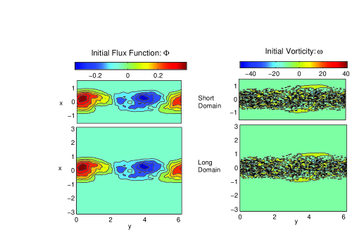
Figure 1: The initial conditions used for the simulations. The perturbations are localized away from the radial boundaries and are identical for the periodic-BC and wall-BC runs.

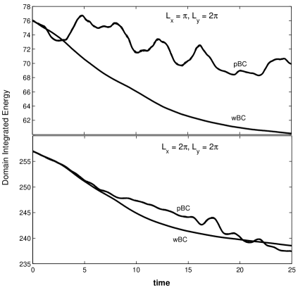
Figure 2: The total energy (in arbitrary units) in the SB as a function of time (in units of $\Omega_{0}^{-1}$). In the upper panel, the size of the SB is $L_{x}=\pi$ and $L_{y}=2\pi$ and the result of the calculation with periodic-BC is compared with the one using wall-BC. In the lower panel, the same is shown for a SB having a double shear-wise extent. In both cases the simulations are started with the same initial conditions, as depicted in Fig. 1 and the evolution is shown during the period in which the typical (of 2-D) decay of the activity has not yet fully set in.

In the upper panel of Fig. 2, we show the evolution of the total energy in the SB of shear-wise extent $L_{x}=\pi$, for periodic-BC and wall-BC, while this figure’s lower panel depicts the same for a SB of double shear-wise extent ($L_{x}=2\pi$). The fluctuations in $\mathfrak{E}$ depicted on the upper panel in periodic-BC simulations are quite dramatic and we have found that they correlate with the action taking place on the boundaries. Clearly, in the smaller SB we have $L_{x}\sim\ell$, that is we are in the situation in which the periodic box size is too small, as we have discussed at the end of the previous section. The dynamics, for the periodic-BC case, is seriously affected by the artificial distortion of the correlation function brought about by the periodic-BC on a too small domain. In contrast, the evolution with wall-BC proceeds smoothly, as the boundary conditions do not allow artificial energy inflow/outflow. The fluctuations in the periodic-BC case have a time scale related to the period time of the shearing box given by

$$T=\frac{L_{y}}{\Omega_{0}qL_{x}},$$

as we can clearly see from the time behavior of the surface term (not shown). This behavior is also apparent in Fig. 2, but is less prominent and clear. We reason that these fluctuations are driven by successive passages of the developed coherent structures (vortices, in this case) in the imaginary neighboring boxes. The vortices that appear in all our simulations are actually somewhat tighter than the initial vorticity perturbation extent, suggesting that $\ell\sim 1$ or so. We also see this trend played out in the lower panel, however an important difference is clearly apparent. The domain size is now $L_{x}\hbox{\raise 1.50696pt\hbox to0.0pt{$>$\hss}\lower 2.58334pt\hbox{$\sim$}\ }6$, that is, considerably larger than $\ell$. In this case, the periodic-BC do not induce very significant spurious energy exchange with the exterior and consequently the fluctuations of the SB energy content are rather mild. We may reasonably conjecture that a calculation with $L_{x}\gg\ell$ would reveal no difference between the pBC and wBC curves.

The longtime decay, which we have mentioned above as being typical in a 2-D problem of this kind, is obviously due to the bulk dissipation embodied in the term $\cal D$. We comment again that the effects we wished to demonstrate in the above numerical experiment can not be significantly altered by the third (vertical) direction because the key factor responsible for them is the boundary condition in the shear-wise direction.

In summary, our numerical experiments show that the type of boundary conditions, coupled with the box size, adopted in investigations of local disk turbulence have important implications on the physical results. When one considers the total energy of disturbances within the formalism of the SB equations, we note that the total energy $\mathfrak{E}$ fluctuates dramatically on account of the injection/extraction of energy across the boundaries when the size of the box is not large enough as compared to the relevant injection scale. It is thus impossible to see how a SB simulation with periodic-BC can reveal any dynamical behavior that is relevant to a true accretion disk, in which $\ell$ has to be at least of the disk thickness size.

7 Discussion and Summary

Based on the arguments of the previous sections we are led to conclude that existing SB calculations, done with periodic-BC in the fixed-flux as well as zero-flux cases, suffer from some serious inconsistencies and problems. These inconsistencies make these calculations quite unreliable for their purpose - finding the mechanism of and quantitatively estimating the turbulent angular momentum transport and energy dissipation in accretion disks. As we have discussed in this paper, the problems stem from the limitations of the box scale, insufficient resolution of the numerics, unjustified symmetry properties (due to periodic-BC) and, as an additional consequence of periodic-BC and limited box size, the possibility of unrealistic energy sources (sinks), which can seriously interfere with the dynamics.

In the fixed-flux case the linear MRI gives rise to a supercritical transition. In this case the SB calculations with periodic-BC manifest channel flows, resulting from the nonlinear exponential growth of the CM, whose problematic nature arises not only from their shear-wise symmetry but also the fact that the linear instability appears to be more involved than just the one comprising of a linear superposition of the CM. The zero-flux simulations in the same SB setup do not allow for CM, but they suffer from all the other difficulties. Indeed, also zero-flux numerical calculations, when tested for convergence (most recently those of Fromang & Papaloizou 2007), indicate that in the ideal case $\alpha$ (a measure for the angular momentum transport) decreases steadily with increasing resolution. Moreover, in the zero-flux case a dynamo action must be invoked and the MRI is thought to play a role in it. But it is not clear how such an intricate self-sustained process, in which a subcritical transition, similar to the one occurring in hydrodynamic shear flows (see ROP07), can be faithfully uncovered by SB periodic-BC simulations, with their problems, as discussed in this paper.

KPL07 conjectured that the fixed-flux case is probably irrelevant to accretion disks, but clearly accretion disks exist that are threaded by external fields (like, e.g., those around young stellar object, see Shu et al. 2007). Moreover, Pessah, Chan & Psaltis (2007) claim the opposite, i.e. that MRI related angular momentum transport can only occur in disks threaded by strong ($\sim$ equipartition value) fields, basing this conclusion on their numerical simulations. In any case, even if the ultimate development of the magnetic field in the disk makes its geometry inside very involved, this fact cannot annihilate the external field whose lines must close through the disk. It seems, therefore, more likely that the apparent almost linear dependence of $\alpha$ on $B_{z}$ in some SB fixed-flux simulations is simply due to the non-reliability of these calculations. Moreover, SB zero-flux calculations also suffer from most of the same difficulties as the fixed-flux ones (as discussed above).

The most recent numerical studies using the SB with periodic-BC in both fixed-flux and zero-flux case have incorporated explicit $\rm Re$ and ${\rm Re}_{m}$ (that is, physical non-zero viscosity and resistivity) and studied the dependence of the angular momentum transport (or $\alpha$) on these non-dimensional numbers. As we have indicated before, this approach can yield valuable information. Lesur & Longaretti (2007) and Fromang et al. (2007) have reported that $\alpha\propto{\rm P}_{m}^{\kappa}$ with $\kappa>0$. We have shown earlier, using asymptotic semi-analytical techniques, (Umurhan, Menou & Regev, 2007) that such scaling can be naturally expected for ${\rm P}_{m}\ll 1$, and also found that $\kappa$ depends on the boundary conditions (URM07). Our work was done for fixed-flux conditions and in a thin-gap mTC setup (which eliminates the shear-wise invariant CM). However, in general, any dependence of the angular momentum transport on a positive power of ${\rm P}_{m}$ makes the role that the MRI takes as the driver of angular momentum transport in astrophysical disks with such astronomical Reynolds numbers rather doubtful (at least in the fixed-flux case, where it is considered to be the sole driver).

Laboratory experiments have so far not yielded any conclusive indications of MRI driven turbulence, save for the case in which relatively strong azimuthal fields are applied (Hollerbach & Rüdiger 2005; Stefani et al. 2006; Szklarski & Rüdiger 2007). In thin accretion disks, however, strong toroidal (or any other, for that matter) magnetic fields cause significant magnetic pressure and are likely to be inappropriate for accretion disks in the thin, rotationally supported, disk limit.

It is not easy to answer the question, what kind of numerical scheme or which setup is best suited for the problem? In any case, it is not clear what is less appropriate for local numerical studies of accretion disks: wall-BC or periodic-BC in the SB. We believe that the use of periodic-BC, especially in the radial direction, suffers from serious problems unless the power in the perturbation fields is localized away from the boundaries of the system (Dubois et al. 1999, Davidson 2004).

We think that if one wants to extract reliable physical information on the local nature of MHD turbulence in which shear is instrumental, on scales from the dissipation one and up to well into the inertial range, it is likely that mrpC (e.g., ROP07) or mTC (e.g., Liu, Goodman & Ji 2006; Obabko, Cattaneo & Fischer 2006) in a thin-gap setup are more appropriate. There certainly are no walls in accretion disks, but wall-BC calculations of this kind can, at least, be made mathematically consistent and physically sound. One may think that periodic-BC (which are also not realistic for accretion disks) are better suited, but as we have shown SB calculations with periodic-BC suffer from difficulties and inconsistencies for this problem, mathematical as well as physical.

It seems to us that the logical approach to the accretion disk angular momentum transport problem should thus consist of:

1. mathematically and physically sound calculations, most likely in the mrpC or mTC thin-gap setups, for the purpose of learning about the detailed local properties of MHD turbulence (its energy spectrum, correlations etc.);

2. devising a turbulence model, based on the above, so as to replace the $\alpha$ model;

3. global calculations employing the above turbulence model(s) and various boundary conditions, giving rise to accretion disk models that can be confronted with observations.

Regarding the first item, it has to be kept in mind that the saturation mechanism may perhaps be different from the case when there are no physical boundaries (see Knobloch & Julien 2005, who have performed an asymptotic MRI analysis, but for a developed state, far from marginality). The hope is, however, that this should not affect too much the local properties of the MHD turbulence.

The previously mentioned approach of performing global calculations with low Reynolds numbers (e.g., Kérsale et al. 2005) are also useful as complementary studies, in which the dependence of the results on relevant non-dimensional numbers can be uncovered. In any case, any numerical study must be controlled, in the sense that one can faithfully (that is, in a numerically resolved way and without introducing any a-priori periodicity of disturbance correlations) experiment with the relevant mathematical properties (e.g., BC, symmetries) and physical quantities (e.g., viscosity, resistivity) and uncover their effects. Schemes including hyper-viscosity, which are routinely used in numerical turbulence studies, may be employed, but this non-trivial tool must be used with proper care. Global quantities (like the energy) must obviously also be monitored and their development fully understood.

The problem of angular momentum transport in accretion disks, especially if MHD turbulence in a non-isotropic strongly sheared medium is the physical mechanism responsible for it, is extremely difficult and involved. This work, as well as that of KPL07 and others, indicates that the understanding gained so far from SB and other numerical simulations seems unfortunately not to be adequate enough to provide a viable physical prescription that can be effectively used in modeling accretion disks, beyond the old $\alpha$-viscosity parametrization. It seems that only an extensive and coherent program, of the kind that has been undertaken in the turbulent dynamo problem (see Schekochihin et al. 2007), is likely to lead to significant progress. In such a program a massive numerical effort is indispensable, but we would like to stress, in concluding, that analytical (asymptotic or other) approaches can also be very useful in guiding the numerical and laboratory work and better understanding the underlying physics.

8 Acknowledgements

We thank Kristen Menou for his comments and suggestions and Amos Ori for a useful discussion. We gratefully acknowledge Bruno Coppi for pointing out to us his relevant work and for sharing with us some of his deep understanding and insight on the subjects of this paper. Michael Mond shared with us the results of his research, which is in progress, read the manuscript and commented on it. We are grateful to him for this. Finally, we thank Fausto Cattaneo and Aleksandr Obabko who kindly showed us, prior to publication, the results of their extensive high-resolution simulations and discussed them with us.

References

- (1) Balbus, S. A. 2003, ARA&A, 41, 555
- (2) Balbus, S. A. & Hawley, J. F. 1991, ApJ, 376, 214
- (3) Balbus, S. A., & Hawley, J. F. 1998, Rev. Mod. Phys., 70, 1
- (4) Balbus, S. A., Hawley, J. F., & Stone, J. M. 1991, ApJ, 476, 76
- (5) Biskamp, D. 2003, Magnetohydrodynamic Turbulence (Cambridge)
- (6) Brandenburg, A., & Donner, K. J. 1997, MNRAS, 288, L29
- (7) Blackman, E. G., & Field, G. B. 2000, ApJ, 376, 534, 984
- (8) Boldyrev, S., & Cattaneo, F. 2004, Phys. Rev. Lett., 92, 144501
- (9) Cattaneo, F., & Hughes, D. W. 1996, Phys. Rev., 54, 4532
- (10) Cattaneo, F., & Tobias, S. M. 2005, Phys. Fluids, 17, 127105
- (11) Chandrasekhar, S. 1960, Proc. Natl. Acad. Sci., 46, 53
- (12) Chandrasekhar, S. 1961, Hydrodynamic and Hydromagnetic Stability (Oxford)
- (13) Coppi, B., & Keyes, E. A. 2003, ApJ, 595, 1000
- (14) Davidson, P. A., 2004, Turbulence: An Introduction for Scientists and Engineers (Oxford)
- (15) Dubois, T., Jauberteau, F., & Temam, R. 1999, Dynamic Multilevel Methods and the Numerical Simulation of Turbulence (Cambridge)
- (16) Fromang, S., & Papaloizou, J. 2007, A&A, 476, 1113
- (17) Fromang, S., Papaloizou, J., Lesur, G., & Heinemann, T. 2007, A&A, 476, 1123
- (18) Gammie, C. F., & Balbus, S. E. 1994, MNRAS, 260, 138
- (19) Gardiner, T. A., & Stone, J. M. 2005, AIP Conf. Proc., 784, 475
- (20) Goldreich, P., & Lynden-Bell, D. 1965, MNRAS, 130, 125
- (21) Goodman, J., & Xu, G. 1994, ApJ, 432, 213
- (22) Grinstein, F.F., Margolin, L. G., & Rider, W. J., 2007, Implicit Large Eddy Simulation: Computing Turbulent Fluid Dynamics, (Cambridge)
- (23) Hollerbach, R., & Rüdiger, G. 2005, Phys. Rev. Lett., 95, 124501
- (24) Hawley, J. F. 2001, ApJ, 554, 534
- (25) Hawley, J. F., & Balbus, S. A. 1991, ApJ, 376, 223
- (26) Hawley, J. F., Gammie, C. F., & Balbus, S. A. 1995, ApJ, 440, 742
- (27) Ji, H., Goodman, J.,& Kageyama, A. 2001, MNRS, 325, L1
- (28) Kersalé E., Hughes, D. W., Ogilvie, G. I., Tobias, S. M., & Weiss, N. O. 2004, ApJ, 602, 892
- (29) Kersaleé E., Hughes, D. W., Ogilvie, G. I., & Tobias, S. M. 2006, 638, 382
- (30) King, A. R., Pringle, J. E., & Livio, M. 2007, MNRS, 376, 1740 (KPL07)
- (31) Knobloch, E., & Julien, K. 2005, Phys. Fluids, 17, 094106
- (32) Liu, W., Goodman, J., & Ji, H. 2006, ApJ, 643, 306
- (33) Liu, W., Goodman, J., & Ji, H. 2007, Phys. Rev. E, 76, 016310
- (34) Liverts, E. & Mond, M. 2007, private communication
- (35) Lesur, G., & Longaretti, P.-Y. 2007, MNRAS, 378, 1471
- (36) Lynden-Bell, D., & Pringle, J.E. 1974, MNRAS, 168, 603
- (37) Moffatt, H. K. 1978, Magnetic Field Generation in Electrically Conducting Fluids (Cambridge)
- (38) Noguchi, K., Pariev, V. A., Colgate, S. A., Beckley, H. F., & Nordhaus, J. 2002, ApJ, 575, 1151
- (39) Obabko, A., Cattaneo, F., Fischer, P. 2006, APS abstract #BP1.101
- (40) Oran, E. S., & Boris, J. P. 1993, Comput. Phys., 7, 523
- (41) Parker, E. N. 1979, Cosmical Magnetic Fields (Oxford)
- (42) Pessah, M. E., Chan, C-k., & Psaltis, D. 2007, ApJ, 668, L51
- (43) Pouquet, A., Rosenberg, D., & Clyne, R. 2002, in Statistical Theories and Computational Approaches to Turbulence, Y. Kaneda & T. Gotoh eds, p. 3 (Springer)
- (44) Pope, S. B. 2000, Turbulent Flows (Cambridge)
- (45) Prendergast, K. H. & Burbidge, G. R., 1968, ApJ, 151, L83
- (46) Rincon, F., Ogilvie, G. I. & Proctor, M. R. E. 2007, Phys. Rev. Lett., 98, 254502
- (47) Rüdiger, G., & Hollerbach, R. 2007, Phys. Rev. E, 76, 068301
- (48) Sano, T., & Inutsuka, S., 2001, ApJ, 561, L179
- (49) Sano, T., & Stone, J. M. 2002, ApJ, 570, 314
- (50) Sano, T., Inutsuka, S. I., Turner, N. J., & Stone, J. M. 2004, ApJ, 605, 321
- (51) Schekochihin, A.A., Cowley, S.C., Taylor, S.F., Maron, J.L. & McWilliams, J.C. 2004, ApJ, 612, 276
- (52) Schekochihin, A.A. et al. 2005, ApJ, 625, L115
- (53) Schekochihin, A.A., & Cowley, S.C. 2006, in Magnetohydrodynamics: Historical Evolution and Trends, S. Molokov et al. eds, p. 85 (Springer) arXiv:astro-ph/0507686
- (54) Schekochihin, A. A. et al. 2007, New J. Phys. ,9, 300
- (55) Shakura, N. I., & Sunyaev, R. A. 1973, A&A, 24, 337
- (56) Shu, F. H., Galli, D., Lizano, S., Glassgold, A. E., & Diamond, P. H. 2007, ApJ, 665, 535
- (57) Sisan, D. R. et al. 2004, Phys. Rev. Lett., 93, 114502
- (58) Stefani, F. et al. 2006, Phys. Rev. Lett., 97, 184502
- (59) Stone, J. M., Hawley, J. F., Gammie, C. F., & Balbus, S. A. 1996, ApJ, 463, 656
- (60) Szklarski, J., & Rüdiger, G., 2006, AN 327, 844
- (61) Toomre, A. 1964, ApJ, 139, 1217
- (62) Umurhan, O. M., Menou, K., & Regev, O. 2007, Phys. Rev. Lett., 98, 034501
- (63) Umurhan, O. M., & Regev, O. 2004, A&A, 427, 855
- (64) Umurhan, O. M., Regev, O., & Menou, K. 2007, Phys Rev E, 76, 036310 (URM07)
- (65) Velikhov, E. P. 1959, J. Exp. Theor. Phys., USSR, 36, 1398
- (66) Wilcox, D. C. 1998, Turbulence Modeling for CFD, 2-ed. (DCW Industries)