Density correlations in ultracold Fermi systems within the exact Richardson solution

Abstract

We discuss the occupation number correlations in an ultracold system of interacting fermionic atoms. For a system with a special energy-level distribution, viz. two multiply-degenerate levels, explicit expressions for the correlation functions are derived in a canonical approach using the exact ground state wavefunction of the reduced BCS Hamiltonian. We evaluate the correlators numerically for different interaction strength and find analytical expressions in some limiting cases. Due to the underlying fermionic nature of the pairs the occupations are predominantly anti-correlated and their statistics is a multinomial distribution.

I Introduction

Ultracold fermionic gases have attracted considerable attention in theoretical and experimental physics recently. This has been intensified after the experimental successes in creating Bose-Einstein Condensates (BECs) in fermionic clouds. An important step was the development of techniques using magnetically detuned Feshbach resonances Observ_Reson_Ferm , which allow to tune the mutual interaction strength between the fermions over a wide range. This novel opportunity to look at a transition from a weakly attractive Bardeen-Cooper-Schrieffer (BCS) state to a strongly attractive BEC in one and the same system makes it interesting from a many-body point of view (see grimm2007 for a recent review). Measurements of the interaction strength of a fermionic gas near a Feshbach resonance were made by time-of-flight expansion experiments Bourdel:03 . The collective excitations showed a strong dependence on the coupling strength as was shown experimentally Bartenstein:04 ; Kinast:04 . Other experiments observed condensation Regal:04 ; Zwierlein:04 and the spatial correlations Greiner:04 of the fermionic atom pairs in the full crossover regime. Using a spectroscopic technique the pairing gap was measured directly denschlag:04 . The remarkable result was that the gap values were found in good agreement with a simple BCS expression in the whole crossover regime.

One way to access the nature of the many-body state is to consider its statistics. A number of works proposed to use noise and higher-order correlations to probe the many-body states of ultracold atoms lukin:04 ; budde:04 ; meiser:04 ; lamacraft05a ; belzig_schroll_bruder . For the BEC-BCS transition the density and spin structure factor was calculated buechler:04 . Schemes to measure the spatial pairing order interferometrically were proposed based on correlations in different output channels Carusotto:04 . To look at pairing fluctuations of trapped Fermi gases has been proposed in viverit:04 . Experimentally in grimm:04 the spatial structure of an atomic cloud was observed directly. This enables to determine the density fluctuations for example by repeating the experiment many times or by extracting densities at different positions in a homogeneous system to obtain the statistics. The shot noise of an atomic beam has been experimentally investigated both in bosonic and fermionic systems foelling:05 ; aspect2005 ; greiner:05 ; bloch2006 ; esteve2006 ; aspect2007 ; porto2007 . Further aspects of full counting statistics in ultracold atomic systems are discussed in the experimental work in Ref. esslinger2005, and the theoretical papers lamacraft05b ; meystre ; moritz ; svistunov ; galitski:07 .

Recently, Amico and coworkers have considered the exact solution of the BCS model in some systems using the algebraic Bethe-Ansatz amico:xx . Explicit expressions for average occupations and the number correlators have been obtained. Subsequent work has tackled the problem numerically and found the Bethe-Ansatz solution to be numerically expensive faribault:07 . The approach to the occupation number correlators through the Richardson solution, which we develop below, can lead to a numerically less expensive method in some cases. A recent review of the limit of large particle numbers of the Richardson solution can be found in dukelsky:04, .

In a previous publication, we have calculated the full statistics of particle number fluctuations in ultracold fermionic gases using a grand-canonical approach belzig_schroll_bruder . The idea was to consider a ‘bin’, i.e., a small subsystem of a homogeneous gas which contains a macroscopic number of particles, such that the surrounding atomic gas serves as the particle reservoir. Fluctuations can in principle be accessed experimentally by performing a series of measurements of the number of particles in the subsystem at a fixed interaction constant, or by considering different bins of the system. The statistics in the whole BCS-BEC crossover is hence obtained if one sequentially performs such sets of measurements from small to large interaction constant. Due to its effective single-particle form one can calculate correlation functions using the (grand-canonical) Bardeen-Cooper-Schrieffer (BCS) ground state solution Superconductivity . It was found that the BCS-BEC transition yields a crossover in the statistics of the particle number. Fluctuations around the average particle number are strongly suppressed on the BCS side and the statistical distribution is binomial. On the BEC side, fluctuations are strongly enhanced and are described by a Poissonian statistics.

Since real ultracold gases consist of a finite number of particles, the grand-canonical approach may be inappropriate. In this article we thus focus on particle-number correlations obtained from the exact ground state using the methods developed by Richardson Exact_Eigenstates1 ; Exact_Eigenstates2 ; Introduction_Richardson ; Numerical_Study ; Number_Dependence ; Application_Isotopes_Lead . The Richardson ground state is an eigenstate of the total particle number operator $\hat{N}=\sum_{i}\hat{n}_{i}$ and thus allows a canonical treatment of the system. Due to the complexity of the Richardson solution, we restrict our investigations to a simplified level distribution consisting of two multiply degenerate energy levels. This allows us to compare explicitly the thermodynamic limit of the exact ground state and the approximate BCS solution. Some model-independent properties of the statistics can be obtained in the limiting cases of vanishing or very strong interaction.

Although this is a toy model, it is relevant for a number of experimental situations. First, we note that the large degree of control possible in ultra-cold atomic systems, e.g. by using optical lattices or atomic chips, will make it possible to produce few-level systems, which can be loaded with a fixed number of fermions in a controlled way. Experiments on particle number correlations in such systems will be described bny the theory developed below. Our results apply equally well to level configurations, in which only two groups of levels are relevant. The level spacing within each group has to be smaller than the interaction constant; the transition from weak to strong coupling appears for interactions of the order of the energy spacing between the groups. We would also like to mention, that the results obtained below for the strongly interacting limit are valid for any level configuration, in which the maximal level spacing is smaller than the interaction constant. Hence, we believe that systems corresponding to the model we study can be experimentally produced, or, at least, some predictions can be tested in the limiting case of a strong interaction in an arbitrary level configuration.

II Properties of the exact solution

II.1 General case

We start by recalling the basic properties of the Richardson solution to the reduced Hamiltonian Spectros_Ultra_Grain ; Introduction_Richardson . The Hamiltonian in second quantization and momentum space has the form

$$H=\sum_{f}2\epsilon_{f}\hat{n}_{f}-g\sum_{ff^{\prime}}\hat{b}_{f}^{\dagger}\hat{b}_{f^{\prime}}^{\phantom{\dagger}}~{},$$ (1)

where $\hat{b}_{f}=\hat{c}_{f\downarrow}\hat{c}_{f\uparrow}$ are hard-core bosonic annihilation operators. The reduced Hamiltonian captures only the scattering fermions which occur in time-reversed states. It is therefore possible to express the particle number operator totally in terms of $\hat{b}$-operators:

$$\hat{n}_{f}=\frac{\hat{c}_{f\uparrow}^{\dagger}\hat{c}_{f\uparrow}^{\phantom{\dagger}}+\hat{c}_{f\downarrow}^{\dagger}\hat{c}_{f\downarrow}^{\phantom{\dagger}}}{2}=\hat{b}_{f}^{\dagger}\hat{b}_{f}^{\phantom{\dagger}}~{}.$$ (2)

This is true only in the subspace of fully paired states, to which we will restrict ourselves here and in the following. The $J$-th (with $J=1$: ground state, $J=2$: first excited state, etc.) $N$-particle eigenstate of (1) has the form

$$|\Psi_{N}^{(J)}\rangle=\sum_{f_{1}\ldots f_{N}}\varphi^{(J)}(f_{1},\ldots,f_{N})\prod_{\nu=1}^{N}b_{f_{\nu}}^{\dagger}|0\rangle~{}.$$ (3)

Because of $(b_{f}^{\dagger})^{2}=0$ only those terms contribute to the sum for which all of the indices $f_{1},\ldots,f_{N}$ are distinct. The coefficient is given by

$$\varphi^{(J)}(f_{1},\ldots,f_{N})=C\sum_{P}\prod_{\nu=1}^{N}\frac{1}{2\epsilon_{f_{\nu}}^{\phantom{J}}-E_{P(\nu)}^{(J)}}~{},$$ (4)

where $\sum_{P}$ denotes the sum over all permutations $P(i)$. The normalization constant $C$ can be determined applying a standard determinant method Exact_Eigenstates2 . The quasi-energies $E_{\nu}^{(J)}$ in Eq. (4) are the solutions of the set of coupled root equations

$$1-\sum_{f}^{U}\frac{g}{2\epsilon_{f}-E_{\nu}}+\sum_{\nu^{\prime}\neq\nu}^{N}\frac{2g}{E_{\nu^{\prime}}-E_{\nu}}=0,\quad\nu=1\ldots N~{}.$$ (5)

In general, the $E_{\nu}^{(J)}$ are complex quantities, however they always appear in complex-conjugate pairs. The corresponding energy eigenvalue is given by

$$\varepsilon_{N}^{(J)}=\sum_{\nu=1}^{N}E_{\nu}^{(J)}~{},$$ (6)

and is thus real, as required.

II.2 The two-level model

We will now consider the special configuration involving $N$ particles in two multiply-degenerate energy levels $\epsilon_{0}$ and $\epsilon_{1}$ with the degeneracies $\Omega_{0}$ and $\Omega_{1}$, respectively . In the following the subscripts $0$ and $1$ will refer to one of the lower levels and one of the upper levels, respectively. The coefficients $\varphi$ from Eq. (4) can be expressed in terms of a single variable $\nu$ that indicates the amount of particles in the upper level $\epsilon_{1}$ Exact_Eigenstates1 : $\varphi^{(J)}(f_{1},\ldots,f_{N})\to\varphi^{(J)}(\nu)$. This leads to a simplification in finding the Richardson solution. Introducing the abbreviations

$$\omega_{\nu} = 2N\epsilon_{0}+2\nu(\epsilon_{1}-\epsilon_{0})-g\nu(\Omega_{1}-\nu+1)$$ (7)

$$-g(N-\nu)(\Omega_{0}-N+\nu+1)~{},$$

$$A_{\nu} = g(N-\nu)(\Omega_{1}-\nu)~{},$$ (8)

$$B_{\nu} = g\nu(\Omega_{0}-N+\nu)~{},$$ (9)

the coefficients are determined by the continued-fraction formula

$$\varphi^{(J)}(\nu)=\cfrac{B_{\nu}\varphi^{(J)}(\nu-1)}{\omega_{\nu}-\varepsilon_{N}^{(J)}-\cfrac{A_{\nu}B_{\nu+1}}{\omega_{\nu+1}-\varepsilon_{N}^{(J)}-\ldots{{}-\cfrac{A_{N-1}B_{N}}{\omega_{N}-\varepsilon_{N}^{(J)}}}}}\,.$$ (10)

$\varphi^{(J)}(0)$ has to be extracted from the normalization condition

$$\sum_{\nu=0}^{N}{\Omega_{0}\choose N-\nu}{\Omega_{1}\choose\nu}\big{[}{\varphi^{(J)}}(\nu)\big{]}^{2}=1\;.$$ (11)

One can find an expression for the total energy (6) appearing in Eq. (10) directly from the root equation

$$\omega_{0}-\varepsilon_{N}=-\cfrac{A_{0}B_{1}}{\omega_{1}-\varepsilon_{N}-\cfrac{A_{1}B_{2}}{\omega_{2}-\varepsilon_{N}-\ldots{{}-\cfrac{A_{N-1}B_{N}}{\omega_{N}-\varepsilon_{N}}}}}\,,$$ (12)

without having to resort to the quasi-energies from Eqs. (5).

In the following, we will use the level spacing $\epsilon_{1}-\epsilon_{0}=1$ as our energy scale. The only (dimensionless) parameter left to characterize the system is the ratio between the interaction constant $G$ and the level spacing.

The model of two highly-degenerate levels is clearly an artificial model, which cannot be mapped to generic many-particle systems. However, we believe the model is nonetheless relevant also for experimental realizations due to two reasons. First, we show below that deviations of the occupation number correlators from a simple BCS mean-field treatment are relevant and can be detected in not too large systems. In experimental realizations of interacting Fermi systems in ultracold atomic gases an unprecedented variability of system parameters has been experimentally demonstrated grimm2007 . We therefore hope that our investigation will stimulate experimental efforts to create few-particle strongly-interacting systems and study the effects we predict below. Second, within the same reasoning we believe that the large variability of tailoring atom systems in (magneto-)optical traps or via atomic chips will make it possible to create an artificial highly-degenerate two-level system and to use it to study in a controlled manner the transition to the thermodynamic limit in a particularly simple system, as we predict here.

II.3 Example

We want to illustrate some characteristics of the Richardson solution by means of a simple setup within the two-level model. We consider, therefore, a system of two hard-core bosons in two threefold degenerate levels ($\Omega_{0}=\Omega_{1}=3$) of energy $\epsilon_{0}=0$ and $\epsilon_{1}=1$. Figure 1 shows the three root solutions of Eq. (12) as a function of the interaction $g$. Obviously, in the non-interacting limit at $g\ll 1$, the energies reduce to the bare pair energies 0, 2 and 4, corresponding to the case that $\nu=0,~{}\nu=1$ and $\nu=2$ particles respectively are in the upper level. With increasing interaction $g\approx 1$, the ground state and first excited state energies are lowered continuously, whereas the second excitation energy approaches $\varepsilon_{2}^{(3)}=2$ and is then independent of the interaction constant $g$.

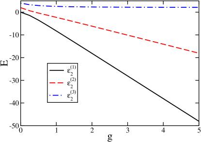
Figure 1: (Color online) Development of the ground state and first and second excited state energy vs. interaction constant $g$ for a simple two-boson system. The two levels at $\epsilon_{0}=0$ and $\epsilon_{1}=1$ are both threefold degenerate.

In the following, we concentrate our investigations on the behavior of the ground state. Figure 2 shows the behavior of the many-body occupation $\big{[}\varphi^{(1)}(\nu)\big{]}^{2}$ as a function of $g$. At vanishing interaction only the lower three energy levels at $\epsilon_{0}$ are occupied. From the normalization condition (11) it thus follows that $[\varphi^{(1)}(0)]^{2}=1/3$, since there are ${3\choose 2}=3$ distinct possibilities to distribute two particles among three levels. The average occupation number of a lower level is hence given by $\langle\hat{n}_{0}\rangle=\frac{2}{3}$. At strong interactions $g\gg 1$, all levels tend to become equally occupied. In this limit, we can therefore neglect the level spacing and consider simply a single energy level with a total a single total degeneracy $\Omega=\Omega_{0}+\Omega_{1}=6$. Equation (11) simplifies to $[\varphi^{(1)}(\nu)]^{-2}={\Omega\choose N}={6\choose 2}=15$, which is independent of $\nu$, and the average particle number of a level is given by $\langle\hat{n}_{0}\rangle=\langle\hat{n}_{1}\rangle=N/\Omega=1/3$. We want to point out here that the equal occupation of all levels in the strong interacting limit is not restricted to this specific level model but rather a general feature of the Richardson ground state.

Figure 2: Many-body coefficient $[\varphi^{(1)}(\nu)]^{2}$ as a function of $g$ for the ground state energy $\varepsilon_{2}^{(1)}$.

For $g\gg 1$ it follows from Eq. (10) and Eq. (12) that the ground state energy approaches

$$\varepsilon_{N}^{(1)}=\omega_{0}-A_{0}\frac{\varphi^{(1)}(1)}{\varphi^{(1)}(0)}\approx 2N\epsilon_{0}-gN(\Omega-N+1)\,,$$ (13)

since $\varphi^{(1)}(1)\approx\varphi^{(1)}(0)$. This useful relation can e. g. be taken as an initial energy guess in the whole interaction regime, when it comes to finding the roots of Eq. (12).

III particle-number correlations: grand-canonical vs. canonical

We address now the correlations following from the exact ground state. We particularly focus on the differences that occur in a canonical treatment compared to applying the grand-canonical BCS solution. At first, we define the particle number cross-correlator between the occupations of levels $f\neq f^{\prime}$

$$g(f,f^{\prime}) := \langle(\hat{n}_{f}-\langle\hat{n}_{f}\rangle)(\hat{n}_{f^{\prime}}-\langle\hat{n}_{f^{\prime}}\rangle)\rangle$$ (14)

$$= \langle\hat{n}_{f}\hat{n}_{f^{\prime}}\rangle-\langle\hat{n}_{f}\rangle\langle\hat{n}_{f^{\prime}}\rangle\,,$$

which represents a direct measure of how much the particle number of level $f$ fluctuates around its mean value in the presence of a fluctuation around the mean value of the particle number of level $f^{\prime}$.

The grand-canonical BCS wavefunction Superconductivity is given by

$$|\textnormal{BCS}\rangle=\prod_{f}\big{(}u_{f}+v_{f}b_{f}^{\dagger}\big{)}|0\rangle~{},$$ (15)

with $v_{f}^{2}=1-u_{f}^{2}=(1-(\epsilon_{f}-\mu)/\sqrt{(\epsilon_{f}-\mu)^{2}+\Delta^{2}})/2$, where $\mu$ is the chemical potential. The mean field $\Delta$ and $\mu$ are fixed by the self-consistency equations

$$\Delta=-g\sum_{f}u_{f}v_{f}~{},~{}\bar{N}=2\sum_{f}v_{f}^{2}~{}.$$ (16)

The simplification by the mean field Ansatz, that is the reduction of the many-body interaction to an effective one-body interaction, has a direct consequence on cross-correlations: Since (15) is a product state the different level occupations are uncorrelated and, hence, $g(f,f^{\prime})=0$. As we will see in the following sections, the correlations will be non-zero if the many-body interaction is taken into account beyond the mean-field approach.

Due to the operator identity $\hat{n}_{f}=\hat{n}_{f}^{l}$ for $l=1,2,...$ in the subspace of paired particles, the auto-correlation function of a level, Eq. (14) with $f=f^{\prime}$, is totally determined by its average particle number and thus does not contain any additional information. In the following, we will therefore concentrate on the investigation of exact average particle numbers and exact particle number cross-correlators in the form of Eq. (14).

III.1 Exact correlators in the two-level model

We now determine the explicit form of the particle number cross-correlator (14) in the two-level model. We only have to consider three different kinds of correlators, since all degenerate levels are equivalent. If two levels of the same energy are distinct, we indicate this by priming one of the indices labeling the energy of the level. The three different cases take the form

$$g(0,0^{\prime}) = \langle\hat{n}_{0}\hat{n}_{0^{\prime}}\rangle-\langle\hat{n}_{0}\rangle^{2}$$ (17)

$$g(0,1) = \langle\hat{n}_{0}\hat{n}_{1}\rangle-\langle\hat{n}_{0}\rangle\langle\hat{n}_{1}\rangle$$ (18)

$$g(1,1^{\prime}) = \langle\hat{n}_{1}\hat{n}_{1^{\prime}}\rangle-\langle\hat{n}_{1}\rangle^{2}$$ (19)

with (assuming that $N\leq\Omega_{0},~{}\Omega_{1}$)

$$\langle\hat{n}_{0}\hat{n}_{0^{\prime}}\rangle = \sum_{\nu=0}^{N-2}{\Omega_{0}-2\choose N-2-\nu}{\Omega_{1}\choose\nu}\left[\varphi^{(1)}(\nu)\right]^{2}\,,$$ (20)

$$\langle\hat{n}_{0}\hat{n}_{1}\rangle = \sum_{\nu=1}^{N-1}{\Omega_{0}-1\choose N-1-\nu}{\Omega_{1}-1\choose\nu-1}\left[\varphi^{(1)}(\nu)\right]^{2}\,,$$

$$\langle\hat{n}_{1}\hat{n}_{1^{\prime}}\rangle = \sum_{\nu=2}^{N}{\Omega_{0}\choose N-\nu}{\Omega_{1}-2\choose\nu-2}\left[\varphi^{(1)}(\nu)\right]^{2}$$

and

$$\langle\hat{n}_{0}\rangle = \sum_{\nu=1}^{N}{\Omega_{0}-1\choose N-1-\nu}{\Omega_{1}\choose\nu}\left[\varphi^{(1)}(\nu)\right]^{2}\,,$$ (21)

$$\langle\hat{n}_{1}\rangle = \sum_{\nu=0}^{N-1}{\Omega_{0}\choose N-\nu}{\Omega_{1}-1\choose\nu-1}\left[\varphi^{(1)}(\nu)\right]^{2}\,.$$ (22)

If we allow particle numbers exceeding one or both degeneracies, the boundaries in the sums appearing in Eqs. (11), (20) and (21) have to be adjusted accordingly.

III.2 Relation to counting statistics

In the two-level model, we are also able to specify the full statistics of the occupation numbers. This quantity can in principle be obtained by measuring repeatedly the occupation numbers and finding the probability $P(n_{f},n_{f^{\prime}})$ that two levels $f$ and $f^{\prime}$ have occupations $n_{f}$ and $n_{f^{\prime}}$. This full statistics can be equivalently expressed through the cumulant generating function $S_{f{f^{\prime}}}(\chi_{f},\chi_{f^{\prime}})=\ln\sum_{n_{f},n_{f^{\prime}}}\exp(i\chi_{f}n_{f}+i\chi_{f^{\prime}}n_{f^{\prime}})P_{f{f^{\prime}}}(n_{f},n_{f^{\prime}})$ belzig_schroll_bruder . The cumulant generating function for hard-core bosons in a fully paired state is given as a function of two counting fields $\chi_{f}$ and $\chi_{f^{\prime}}$:

$$e^{S_{f{f^{\prime}}}(\chi_{f},\chi_{f^{\prime}})} = \langle e^{i(\chi_{f}\hat{n}_{f}+\chi_{f^{\prime}}\hat{n}_{f^{\prime}})}\rangle$$

$$= 1+\langle\hat{n}_{f}\rangle\left(e^{i\chi_{f}}-1\right)$$

$$+\langle\hat{n}_{f^{\prime}}\rangle\left(e^{i\chi_{f^{\prime}}}-1\right)$$

$$+\langle\hat{n}_{f}\hat{n}_{f^{\prime}}\rangle\left(e^{i\chi_{f}}-1\right)\left(e^{i\chi_{f^{\prime}}}-1\right)\,.$$

Consequently, the only correlator which needs to be known to fully determine the CGF is the one in the last line of Eq. (III.2), for which we are able to give explicit expressions here, due to the simplicity of the model.

In the case of non-interacting particles, e.g. hard-core bosons in the BCS mean-field treatment, Eq. (III.2) factorizes according to

$$e^{S_{ff^{\prime}}(\chi_{f},\chi_{f^{\prime}})} = e^{S_{f}(\chi_{f})+S_{f^{\prime}}(\chi_{f^{\prime}})}$$

$$= \left[1+\langle\hat{n}_{f}\rangle\left(e^{i\chi_{f}}-1\right)\right]$$

$$\times\left[1+\langle\hat{n}_{f^{\prime}}\rangle\left(e^{i\chi_{f^{\prime}}}-1\right)\right]\,.$$

This is the CGF of uncorrelated particle numbers. Comparing these general results for the counting statistics with the correlators discussed in the previous subsection we observe that in this special case the counting statistics contains not more information than the correlators alone. Or, in other words, if the correlators Eq. (17)-(19) are known, one can use Eq. (III.2) to calculate the full counting statistics.

III.3 Asymptotic behavior

Before we discuss the general results for an arbitrary interaction constant, we obtain analytical expressions for the correlators in the limiting cases of weak and strong interactions. This is possible since the coefficients (4) can be directly determined from the normalization condition (11) without having to solve the root equation, Eq. (12). In the following, we will assume that $N\leq\Omega_{0},~{}\Omega_{1}$. For $g\ll 1$, Eq. (11) reduces to $\left[\varphi^{(1)}(0)\right]^{-2}={\Omega_{0}\choose N}$. From Eq. (20) and Eq. (21) thus follows

$$g(0,0^{\prime})=-\langle\hat{n}_{0}\rangle^{2}\frac{1-\langle\hat{n}_{0}\rangle}{N-\langle\hat{n}_{0}\rangle}\,,$$ (25)

with the system-size-independent average particle number $\langle\hat{n}_{0}\rangle=N/\Omega_{0}$. The remaining correlators are zero.

For $g\gg 1$ we have correspondingly $\left[\varphi^{(1)}(\nu)\right]^{-2}={\Omega\choose N}$, where $\Omega=\Omega_{0}+\Omega_{1}$. Hence we get

$$g(f,{f^{\prime}})=-\langle\hat{n}\rangle^{2}\frac{1-\langle\hat{n}\rangle}{N-\langle\hat{n}\rangle}\,.$$ (26)

Again $\langle\hat{n}\rangle=N/\Omega$ is the system-size and interaction-constant independent average occupation number of every level. Since it is a feature of the Richardson solution, that all coefficients $\big{[}\varphi^{(1)}(f_{1}\ldots f_{N})\big{]}^{2}$ become equal in the strongly-interacting limit, (26) is a universal property of particle-number correlators, which is valid also for arbitrary level configurations and not only restricted to this simple model.

III.4 The two-level model at half filling

We now discuss the numerical results of the average particle numbers and correlators above as we approach the thermodynamic limit starting from finite system sizes. In the evaluation of e. g. Eq. (20) and Eq. (21), we hence have to assure that the involved quantities scale in the correct manner. The continuum limit is obtained by taking $\Omega\to\infty$, while leaving $\frac{N}{\Omega}$ and $G=g\Omega$ constant Etats_Propres ; Pairing_Limit ; Large_N_Limit . We call $G$ the ‘system-size-independent coupling constant’. Under these assumptions, increasing the particle number will lead to the BCS results in the thermodynamic limit.

At first, we investigate the two-level model at half filling with equal degeneracies of both energy levels, viz. $\Omega_{0}=\Omega_{1}=N$. Figure 3 shows the average particle number in one of the upper levels as a function of $G$ for various system sizes. We can see that there is already a fairly good agreement to the BCS results in the case of only 32 particles. Due to the particle-hole symmetry of the system, the connection between the average particle number of a lower level and an upper level is given by $\langle\hat{n}_{0}\rangle=1-\langle\hat{n}_{1}\rangle$. The average particle numbers in the limits of weak and very strong interactions are system-size independent: for $G\ll 1$, only the lower energy band is occupied. For $G\gg 1$ as mentioned in Sec. II.3, we obtain an equal occupation of all levels.

Figure 3: (Color online) Average particle number of one of the upper levels as a function of $G$ for various system sizes. The black solid lines correspond to the solutions obtained from BCS theory. Note that the self-consistency Eqs. (16) in this case only have real solutions for $G>1$. The average particle number of one of the lower levels follows from $\langle\hat{n}_{0}\rangle=1-\langle\hat{n}_{1}\rangle$.

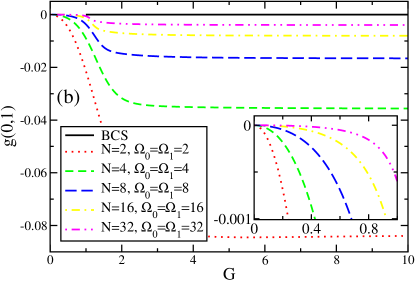
Figure 4: (Color online) $g(0,0^{\prime})=g(1,1^{\prime})$ (upper plot) and $g(0,1)$ (lower plot) as a function of $G$ for various system sizes. The inset shows that, in contrast to $g(0,0^{\prime})$, $g(0,1)$ is always negative in the low-interaction regime.

In Fig. 4 the corresponding correlations are given as a function of $G$. Note that, due to particle-hole symmetry in the half-filled case $g(0,0^{\prime})=g(1,1^{\prime})$. The behavior of the average particle numbers in the strongly-interacting case has a direct influence on the correlations causing $g(0,0^{\prime})$, $g(0,1)$ and $g(1,1^{\prime})$ to become equal in magnitude for a fixed system size. At vanishing interaction, the lacking possibility of reshuffling particles in a fully occupied band leads to zero-correlation. A comparison of the plots in Fig. 4 shows that for a given $N$, the crossover happens over a smaller range of $G$ in the case of $g(0,1)$. Obviously, the fact that all occupations $\nu$ contribute to this correlator - contrary to Eq. (17), where $\nu=N$ only enters through the normalization (11) - leads to a faster saturation with increasing coupling constant.

As a general feature, one finds that the particle number correlators of distinct levels tend to converge to the zero-correlation line of the mean-field approach in the whole interaction regime as one increases the number of particles. A direct indication of the fermionic origin of the hard-core bosons is that, at first sight, in the non-limiting cases $N\neq\infty$ and $G\neq 0$ all correlators are negative, corresponding to anti-correlated particle numbers: Due to the presence of a particle in level $f$, it is less probable to find another particle at the same time in level ${f^{\prime}}$ than in the uncorrelated case. However for $g(0,0^{\prime})$, we observe a range at intermediate interactions, where particles of a certain energy promote other particles to occupy the same level. It also leads to another point of vanishing correlation for $G\neq 0$ and fixed $N$; see Fig. 5. Evaluating $g(0,0^{\prime})$ in second-order perturbation theory shows that this effect starts to occur for $N>2$. There is a resonance effect with a maximum peak value in the positive correlation between 16 and 32 particles. We do not find a positive range for $g(0,1)$. This surprising finding is confirmed analytically by a perturbative calculation in the appendix.

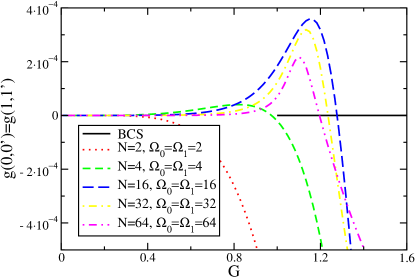
Figure 5: (Color online) Zoom into the region of positive correlations of $g(0,0^{\prime})=g(1,1^{\prime})$ in the weak-coupling range for different system sizes. A positive peak develops around $G=1$ for small systems and becomes maximal for $N\approx 16$. For large system sizes the absolute values become smaller again, but the overall feature sharpens.

III.5 The two-level model away from half filling

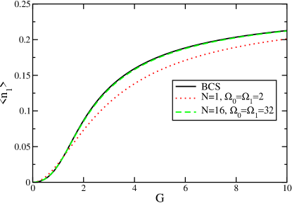
Figure 6: (Color online) Average particle number of one of the upper levels as a function of $G$ for various system sizes in the quarter-filled case $\delta=1/4$. The BCS Eqs. (16) have real solutions for $G>0$ in this case. The average particle number of one of the lower levels follows from $\langle\hat{n}_{0}\rangle=0.5-\langle\hat{n}_{1}\rangle$.

It is also interesting to study the system away from half filling. As an example we now look at the case of quarter filling. Again, we assume that $\Omega_{0}=\Omega_{1}$ and to have a direct comparison to the model at half filling, we chose the same system sizes as in the last example. Because of particle-hole symmetry we have the following relations between filling factors $\delta=N/(\Omega_{0}+\Omega_{1})$ and $1-\delta$. For the average particle numbers

$$\langle\hat{n}_{0}\rangle_{\delta} = 1-\langle\hat{n}_{1}\rangle_{1-\delta}\;,$$ (27)

$$\langle\hat{n}_{1}\rangle_{\delta} = 1-\langle\hat{n}_{0}\rangle_{1-\delta}\;,$$ (28)

and for the correlator

$$g(0,0^{\prime})_{\delta} = g(1,1^{\prime})_{1-\delta}\;,$$ (29)

$$g(1,1^{\prime})_{\delta} = g(0,0^{\prime})_{1-\delta}\;,$$ (30)

$$g(0,1)_{\delta} = g(0,1)_{1-\delta}\;.$$ (31)

In the following, we will consider the case of $\delta=1/4$ (which is therefore equivalent to $\delta=3/4$). The average occupation of one of the upper levels for this case is shown in Fig. 6. The occupation of one of the lower levels is not shown, since it follows from $\langle\hat{n}_{0}\rangle=2\delta-\langle\hat{n}_{1}\rangle$. We see that the saturation at large interaction constant happens at larger $G$ than in the half-filled case (c. f. Fig. 3). Note that here the BCS solution always exists and is indistinguishable from the exact solution already for 16 bosons.

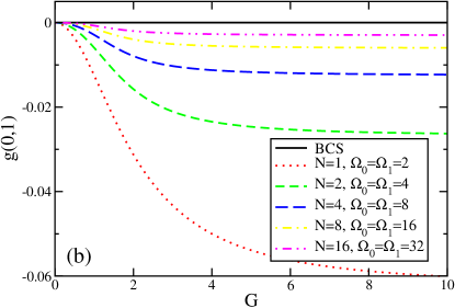
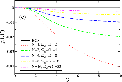
Figure 7: (Color online) $g(0,0^{\prime})$, $g(0,1)$, and $g(1,1^{\prime})$ as a function of $G$ for various system sizes at quarter-filling $\delta=1/4$.

Figure 7 shows that all correlators are now negative and different from each other and approach their limits in the strongly interacting case more slowly than in the half-filled case. $g(0,0^{\prime})$ shows an interesting behavior for vanishing interaction that is caused by the partially occupied lower energy band allowing particles to change states among the lower levels. This leads to a finite value also for $G\approx 0$ and a decay of the correlator with increasing system size, see Eq. (25). It is also remarkable that $g(0,0^{\prime})$ is suppressed by increasing the interaction. Also, in agreement with the perturbative results Eq. (32) the effect of the interaction is of second order in the interaction constant. The other correlators show a similar behavior as in the half-filled case.

IV Conclusion

We have investigated exact particle-number correlations of ultracold fermionic gases in a canonical Ansatz using the Richardson solution. By means of a special configuration involving two degenerate energy levels, correlation functions have been derived and evaluated numerically for different mutual interactions between the atoms and different system sizes. The particle numbers in different levels turn out to be mostly anti-correlated revealing the fermionic origin of the paired particles (the hard-core boson property). Approaching the thermodynamic limit, those correlators decay to zero in the whole interaction regime. This is in agreement with the predictions of BCS theory. In the limit of strong interactions we were able to give closed expressions for the correlations, which are also valid for the general case of arbitrary level configurations. Due to the complex algebraic structure of the Richardson solution, only a comparatively special model could be investigated in this work. The discussion of more general systems remains an open problem. Nevertheless, we believe our predictions can be tested in tailored few-particle systems of interacting fermions, e. g. with atomic chips.

*

Appendix A Perturbative calculation

The Richardson solution and correlators can be found perturbatively in the interaction constant. For $N\leq\Omega_{0},~{}\Omega_{1}$ we find the expression

$$g(0,0^{\prime}) = -\frac{N(\Omega_{0}-N)}{\Omega_{0}^{2}(\Omega_{0}-1)}\left[1-\left(\frac{G}{N}\right)^{2}\frac{\Omega_{1}(\Omega_{0}-N+1)}{2}\right]$$ (32)

$$-\frac{N\Omega_{1}(\Omega_{0}-N+1)}{16\Omega_{0}^{2}(\Omega_{0}-1)}\left(\frac{G}{N}\right)^{4}\Big{[}2N(N-1)(5N-6)-(7N-2\Omega_{0}-7)(3N-\Omega_{0}-2)\Omega_{0}$$

$$+\big{(}13N(N-1)+7\Omega_{0}(2-3N+\Omega_{0})\big{)}\Omega_{1}+2(N-\Omega_{0})\Omega_{1}^{2}\Big{]}\,.$$

For a half-filled band ($N=\Omega_{0}=\Omega_{1}$) the zeroth and the second-order term vanish and the expansion to 6th order yields

$$g(0,0^{\prime})\approx(\frac{1}{16N^{2}}-\frac{1}{8N^{3}})G^{4}+(-\frac{3}{16N^{2}}+\frac{13}{32N^{3}}-\frac{3}{16N^{4}})G^{6}+\mathcal{O}(G^{8})~{}.$$ (33)

The $G^{4}$ term is positive for $N>2$, but gets smaller for increasing $N$. For increasing $G$ the 6th-order term takes over and leads to a negative correlator in the end.

References

- (1) C. A. Regal, M. Greiner, and D. S. Jin, Phys. Rev. Lett. 92, 040403 (2004).
- (2) R. Grimm, in Ultracold Fermi Gases, edited by M. Inguscio, W. Ketterle, and C. Salomon. Proceedings of the International School of Physics ‘Enrico Fermi’, Course CLXIV, Varenna, 20 - 30 June 2006; cond-mat/0703091.
- (3) T. Bourdel, J. Cubizolles, L. Khaykovich, K. M. F. Magalhes, S. J. J. M. F. Kokkelmans, G. V. Shlyapnikov, and C. Salomon, Phys. Rev. Lett. 91, 020402 (2003).
- (4) M. Bartenstein, A. Altmeyer, S. Riedl, S. Jochim, C. Chin, J. Hecker Denschlag, and R. Grimm, Phys. Rev. Lett. 92, 203201 (2004).
- (5) J. Kinast, S. L. Hemmer, M. E. Gehm, A. Turlapov, and J. E. Thomas, Phys. Rev. Lett. 92, 150402 (2004).
- (6) C. A. Regal, M. Greiner, and D. S. Jin, Phys. Rev. Lett. 92, 040403 (2004).
- (7) M. W. Zwierlein, C. A. Stan, C. H. Schunck, S. M. F. Raupach, A. J. Kerman, and W. Ketterle, Phys. Rev. Lett. 92, 120403 (2004).
- (8) M. Greiner, C. A. Regal, C. Ticknor, J. L. Bohn, and D. S. Jin, Phys. Rev. Lett. 92, 150405 (2004).
- (9) C. Chin, M. Bartenstein, A. Altmeyer, S. Riedl, S. Jochim, J. Hecker Denschlag, and R. Grimm, Science 305, 1128 (2004).
- (10) E. Altman, E. Demler, and M. D. Lukin, Phys. Rev. A 70, 013603 (2004).
- (11) M. Budde and K. Mølmer, Phys. Rev. A 70, 053618 (2004).
- (12) D. Meiser and P. Meystre, Phys. Rev. Lett. 94, 093001 (2005).
- (13) A. Lamacraft, Phys. Rev. A 73, 011602 (2006).
- (14) W. Belzig, C. Schroll, and C. Bruder, Phys. Rev. A 75, 063611 (2007).
- (15) H. P. Büchler, P. Zoller, and W. Zwerger, Phys. Rev. Lett. 93, 080401 (2004).
- (16) I. Carusotto and Y. Castin, Phys. Rev. Lett. 94, 223202 (2005).
- (17) L. Viverit, G. M. Bruun, A. Minguzzi, and R. Fazio, Phys. Rev. Lett. 93, 110406 (2004).
- (18) M. Bartenstein, A. Altmeyer, S. Riedl, S. Jochim, C. Chin, J. Hecker Denschlag, and R. Grimm, Phys. Rev. Lett. 92, 120401 (2004).
- (19) S. Fölling, F. Gerbier, A. Widera, O. Mandel, T. Gericke, and I. Bloch, Nature 434, 481 (2005).
- (20) M. Schellekens, R. Hoppeler, A. Perrin, J. Viana Gomes, D. Boiron, A. Aspect, and C. I. Westbrook, Science 310, 648 (2005).
- (21) M. Greiner, C. A. Regal, J. T. Stewart, and D. S. Jin, Phys. Rev. Lett. 94, 110401 (2005).
- (22) T. Rom, Th. Best, D. van Oosten, U. Schneider, S. Fölling, B. Paredes, and I. Bloch, Nature 444, 733 (2006).
- (23) J. Esteve, J.-B. Trebbia, T. Schumm, A. Aspect, C. I. Westbrook, and I. Bouchoule, Phys. Rev. Lett. 96, 130403 (2006).
- (24) T. Jeltes, J. M. McNamara, W. Hogervorst, W. Vassen, V. Krachmalnicoff, M. Schellekens, A. Perrin, H. Chang, D. Boiron, A. Aspect, and C. I. Westbrook, Nature 445, 402 (2007).
- (25) I. B. Spielman, W. D. Phillips, and J. V. Porto, Phys. Rev. Lett. 98, 080404 (2007)
- (26) A. Öttl, S. Ritter, M. Köhl, and T. Esslinger, Phys. Rev. Lett. 95, 090404 (2005).
- (27) A. Lamacraft, Phys. Rev. A 76, 011603(R) (2007).
- (28) A. Nunnenkamp, D. Meiser, and P. Meystre, New J. Phys. 8, 88 (2006).
- (29) A. Kuklov and H. Moritz, Phys. Rev. A 75, 013616 (2007).
- (30) B. Capogrosso-Sansone, E. Kozik, N. Prokof’ev, and B. Svistunov, Phys. Rev. A 75, 013619 (2007).
- (31) P. Nagornykh and V. Galitski, Phys. Rev. A 75, 065601 (2007).
- (32) L. Amico, G. Falci, and R. Fazio, J. Phys. A 34, 6425 (2001); L. Amico, A. Di Lorenzo, and A. Osterloh, Phys. Rev. Lett 86, 5759 (2001); L. Amico and A. Osterloh, Phys. Rev. Lett. 88, 127003 (2002); L. Amico, A. Di Lorenzo, and A. Osterloh, Nucl. Phys. B 614, 449 (2001); L. Amico, A. Di Lorenzo, A. Mastellone, A. Osterloh, and R. Raimondi, Ann. Phys. 299, 228 (2002).
- (33) A. Faribault, P. Calabrese, and J.-S. Caux, arXiv:0710.4865.
- (34) J. Dukelsky, S. Pittel, and G. Sierra, Rev. Mod. Phys. 76, 643 (2004).
- (35) J. Bardeen, L. N. Cooper, and J. R. Schrieffer, Phys. Rev. 108, 1175 (1957).
- (36) R. Richardson and N. Sherman, Nucl. Phys. 52, 221 (1964).
- (37) R. Richardson, J. of Math. Phys. 6, 1034 (1965).
- (38) J. von Delft and F. Braun, Proceedings of the NATO ASI Quantum Mesoscopic Phenomena and Mesoscopic Devices in Microelectronics, edited by I. O. Kulik and R. Ellialtioglu (Kluwer, Dordrecht, 2000), p. 361; arXiv:cond-mat/9911058.
- (39) R. Richardson, Phys. Rev. 141, 949 (1966).
- (40) R. Richardson, Phys. Lett. 14, 325 (1965).
- (41) R. Richardson, Phys. Lett. 5, 82 (1963).
- (42) J. von Delft and D. Ralph, Phys. Rep. 345, 61 (2001).
- (43) M. Gaudin, in Travaux de Michel Gaudin, Modèles exactement résolus (Les Éditions de Physique, France, 1995).
- (44) R. Richardson, J. of Math. Phys. 18, 1802 (1977).
- (45) J. M. Roman, G. Sierra, and J. Dukelsky, Nucl. Phys. B 634, 483 (2002).