Dynamical Transitions of a Driven Ising Interface

Abstract

We study the structure of an interface in a three dimensional Ising system created by an external non-uniform field $H({\bf r},t)$. $H$ changes sign over a two dimensional plane of arbitrary orientation. When the field is pulled with velocity ${\bf v}_{e}$, (i.e. $H({\bf r},t)=H({\bf r-v_{e}}t)$), the interface undergoes a several dynamical transitions. For low velocities it is pinned by the field profile and moves along with it, the distribution of local slopes undergoing a series of commensurate-incommensurate transitions. For large ${\bf v}_{e}$ the interface de-pinns and grows with KPZ exponents.

Introduction:  The study of the structure and properties of surfaces and interfaces in condensed matter is of considerable technological importanceintro1 ; intro2 . Many phase transitions and chemical reactions originate at a surface and their progress in time is often synonymous with the motion of resulting parent- product interfacesintro3 . Often, interfaces undergo structural transitions, like reconstructions and roughening, the study of which have recieved considerable attention in the past because of its importance to a variety of processes like catalysis and surface phase transitionsintro1 ; villain . Surface structure can also be influenced by its dynamics. Consider a simple interface between the ground states of an Ising modelchaikin with nearest neighbor ferromagnetic interactions defined on the $d$ dimensional cubic lattice. The equilibrium, static, interface defined by the height $h({\bf r})$ fluctuates so that the mean squared deviation of $h$ from the average growsbarabasi as $L^{\alpha}$ and $t^{\beta}$ where $L$ is the typical system size, $t$ the time with the exponents $\alpha=(2-d)/2$ and $\beta=2-d/4$. Above $d=2$ the interface remains flat ($\alpha=\beta=0$). On the other hand, a moving interface in this system when driven by an uniform field coarsens such that $\alpha\simeq 2/(d+3)$ and $\beta\simeq 1/(d+2)$.

Motivation:  In a few earlier publicationsphysica ; prl ; pt we have shown that it is, nevertheless, possible to stabilize a macroscopically flat ($\alpha=\beta=0$) but moving interface in this system by using a non-uniform field (see Fig.1) of the form $H({\bf r},t)=H_{0}{\rm tanh}[({\bf r}-{\bf v}_{e}t)\cdot\hat{\bf n}/\chi]$ where the unit vector $\hat{\bf n}$ fixes the orientation of the interface and $\chi$ the (intrinsic) width. In Ref.prl ; pt the properties of such an interface in the two dimensional Ising model was analyzed in detail.

Figure 1: (left) The geometry of our simulation cell. Ising spins are defined over a $14\times 14\times 30$ lattice elongated in the $z$ direction. An external field is imposed which changes sign over a plane $A,B,C$ making angles $\theta$ and $\phi$ with the $x$ and $y$ axes respectively. The plane $A,B,C$ moves to the right with velocity $v_{e}$. (right) A plot of the velocity of the Ising interface $v_{f}$ as a function of $v_{e}$ for two different orientations - (0,2/7)(top) and (2/7,2/7) . Note that for small $v_{e}$, the interface follows the field ($v_{f}=v_{e}$) but gets detached at higher velocities.

The main results of this study were as follows. Firstly, there exists two distinct dynamical phases: for small $v_{e}$, the interface, defined as the locus of all the points where the magnetization $S({\bf r},t)$ changes sign, moves together with the field with velocity $v_{f}=v_{e}$, and its average position is fixed at all times by the plane (line in two dimensions) $z_{0}(x,y)$ over which the field changes sign and the interface remains macroscopically flat. For large $v_{e}>v_{\infty}$, on the other hand, the interface detaches from $z_{0}$ and grows with velocity $v_{\infty}$ essentially driven by an uniform field at the same time coarsening with KPZ exponentsKPZ ; barabasi . The value of $v_{\infty}$ is orientation dependent because the motion of interfaces at low temperatures takes place mainly by flipping the relatively high energy spins occupying corner sites. The interfacial orientation with the largest density of such unstable spins has the highest $v_{\infty}$.

Secondly, the low velocity pinned phase was shown to be rather interesting because it shows an infinite number of structural phases and phase transitions very similar to commensurate-incommensurate transitions in adsorbates on solid surfaceschaikin ; FK ; CI . In the pinned phase, the spatial profile of the field forces the magnetization to follow $H$ as closely as possible. Specifically, the average orientation of the interface is fixed by the orientation of the line $z_{0}$ over which $H$ changes sign. Since the underlying lattice admits only a discrete set of rational orientations, at equilibrium, the interface settles down to the closest rational approximant possible given the finite size of the system. The pinning energy depends on the orientation of the interface relative to the lattice, simple rational fractions being more strongly pinned. Increasing $v_{e}$ has the effect of increasing dynamical noise, and orientations with stronger pinning and shorter relaxation times become preffered. As $v_{e}$ is increased, therefore, an interface with an arbitrary orientation distorts locally so that over most of its length, the orientation conforms to a low order rational fraction. A non-zero density of discommensurationschaikin ; prl ; pt maintains the average orientation of the interface equal to that of $z_{0}$. A plot of the most probable orientation of the interface against the average orientation for any $v_{e}<v_{\infty}$ therefore shows steps corresponding to an incomplete Devil’s staircase structurechaikin ; FK ; prl ; pt .

The purpose of the present Brief Report, is to determine whether these conclusions are valid for the $d=2$ interface in the $d=3$ Ising system and are not an artifact of the reduced dimensionality. Most experimentally relevant interfaces being two dimensional, we believe this to be an essential point which needs to be checked by direct calculation. We show that the general scenario persists even in the higher dimensional case studied here, although there are some special features related to the larger degree of freedom of the two dimensional interface compared to the one dimensional case studied in Refs.prl ; pt . Unlike the former study, where one may make use of a formal mapping of the Ising interface dynamics problem to an Assymetric Exclusion Processbarma to develop efficient numerical codes and obtain useful analytical results, no such mappng is possible for the higher dimensional case and we use standard Monte Carlo simulations using Metropolis update for this problem. The exact nature of the update rule is not expected to influence the qualitative nature of our results. .

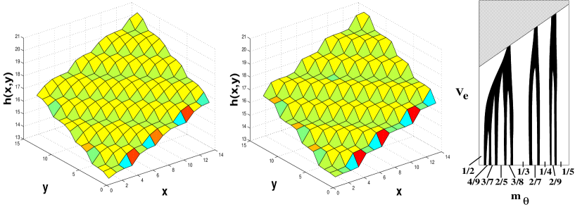
Figure 2: (left (a) and middle (b)) Plots of the averaged interface defined by the locus of zeroes of the magnetization for two different values of $v_{e}=.1$ (left) and $.0125$. The orientation of the interface is ($2/7,2/7$). Note that for small smaller $v_{e}$ the interface is more sharply defined. (right (c) ) A portion of the dynamical phase diagram for a one dimensional interface taken from Ref.pt showing locked (white regions), fluctuating (black regions) and de-pinned (hatched region) phases. Note that an interface with orientation close to (and to the right of) $2/7$ would pass through regions where the most probable orientation shifts to ($1/4$) as the $v_{e}$ is increased.

Mean field results:  When spatial flucutations of the interface are neglected, the velocity of the interface $v_{f}$, defined as the locus of all the points where the magnetization $S({\bf r},t)$ changes sign, is given by the solution of $v_{f}=v_{\infty}{\rm sign}(v_{f}-v_{e})$ at late timesprl . There are two regimes: (a) for small $v_{e}<v_{\infty}$ the interface is pinned by the field and its position coincides with the plane over which the field $\phi$ changes sign so that $v_{f}=v_{e}$ and (b) for $v_{e}>v_{\infty}$, the interface depins and grows with its orientation dependent intrinsic velocity $v_{\infty}$. These mean field results are independent of dimensionality and should hold for Ising systems in any dimensions. We show, indeed, that this is true and the depinning transition, predicted by the mean field calculation persists in $3-d$ (see Fig.1).

Simulation details: Our system consists of $N_{x}(=14)\times N_{y}(=14)\times N_{z}(=30)$ Ising spins arranged in a simple cubic latticelanbin interacting ferromagnetically with their nearest neighbors. The boundary conditions for this system has to be specified with some care since we need to describe, in general, oblique interfaces with arbitrary orientations. We are interested in the low temperature, high field limit, however, which greatly simplifies this task. In this limit, only a few layers of spins immediately adjacent to the interface have any nontrivial dynamics, spins far away from the interface being frozen in the direction of the local external field $H$. We use shifted periodic boundary conditions ensuring that the periodic image of each spin has the same value of $H$ (see Fig 1.). In the ${\bf z}$ direction we have open boundary conditions the exact nature of which is irrelevant as the spins at the two extremeties are, in any case, frozen to the values fixed by the sign of $H$.

A typical run consists of equilibrating the spins in a given $H$, updating $H$ according to the value of $v_{e}$ measured in units of lattice parameter per Monte Carlo step (MCS) and computing the non-uniform magnetization. The value of the magnetization is stored for each time step till the interface traverses the length of the sample. This process is typically repeated $10^{3}$ times and the averaged time dependent magnetization profile is obtained. To obtain the location of the interface the averaged magnetization $S({\bf r},t)$ is fitted to a general hyperbolic tangent profile. The locus of zeroes is the interface. The probability distribution of slopes of this interface is then computed using finite differences and is further averaged over $10^{2}$ independent runs. Therefore, although our system size of $5880$ spins is modest, the scale of our computations is not; a run with a single parameter value needs to be repeated many times to gather sufficient statistics.

Results and Discussion: We begin our discussion of results by considering first the velocity of the interface $v_{f}$ as a function of $v_{e}$. We obtain this from the slope of a plot of the position of the center of mass of the interface as a function of time. Our results for two different orientations of $\hat{\bf n}$ are shown in Fig. 1 (right panel). The depinning transition and saturation of $v_{f}$ to a orientation dependent value of $v_{\infty}$ is clearly visible. The saturation value $v_{\infty}$ depends on the density of steps which, in turn, is a function of the interfacial orientation. Compared to the two dimensional case of Refs.prl ; pt , however, this transition appears to be less sharp. This is, in fact, a finite size effectprl ; lanbin ; the sharp transition is recovered only in the large time limit which is difficult to achieve for our modest system size. Note that the transition is broader for the faster moving interface for which the observation time is shorter.

We concentrate next on the interfacial structure of the pinned interface. The average orientation of the interface is given by the unit vector $\hat{\bf n}$ which may be parametrized by the angles $\theta$ and $\phi$ as shown in Fig. 1 (left panel). We find it more convenient to define the slopes $m_{\theta}=\tan(\theta)$ and $m_{\phi}=\tan(\phi)$. The structure of the interface averaged over many runs is shown in Fig.2 (a) and (b) for two different velocities and for $m_{\theta}=m_{\phi}=2/7$. It is clear from these pictures that the velocity strongly influences the structure, smoothening it on the average. In order to understand better this smoothening process, we compute the probability distribution of the local and instantaneous slope using a resolution window of $5\times 5$ spins. Within this window, the local slope is determined at every intance of time and the data is used to build up the joint probability distribution $P(m_{\theta},m_{\phi})$.

The joint probability distribution $P(m_{\theta},m_{\phi})$ as well as the projected distributions $P(m_{\theta})$ and $P(m_{\phi})$ are plotted in Fig.3 for three different $v_{e}$. In order to understand the sequence of the transitions, we refer to a portion of the dynamical phase diagram in the $v_{e}-m_{\theta}$ plane Fig.2(c). In this figure, the white regions represents the lock-in phases where the most probable orientation locks in to the closest rational slope which may be different from the average slope of the interface. The black regions represent incomensurate states where the the most probable slope is nearly equal to the average slope and the interface dynamically fluctuates between nearby orientations. Finally, the gray region for large $v_{e}$ corresponds to the depinned interface. An interface with a slope $m_{\theta}$ close to but smaller than $2/7$ would first lock-in at $2/7$ for small $v_{e}$ and then to $1/4$ and finally depinn as $v_{e}$ increases. In-between these transitions the interface would be incommensurate.

Figure 3: Projected and two dimensional distributions of the local slope of the interface with an average slope close to $m_{\theta}=2/7$ and $m_{\phi}=2/7$ for various values of $v_{e}$. Left panel shows the probability distribution of the slope $P(m_{\theta})$, the middle panel $P(m_{\phi})$ and the right panel the full two dimensional distribution $P(m_{\theta},m_{\phi})$ for $v_{e}=.2$ (a), $.1$ (b), and $.0125$ (c). Note that in (a), the most probable slope is close to the average slope of the interface. As the velocity is lowered, the interface tends to lock in to a rational slope close to $1/4,1/4$, for which the probability shows the strongest peak (b). As the $v_{e}$ is lowered further, the lock-in slope is a higher order fraction $2/7,2/7$ which is closer to the average orientation of the interface. Large fluctuations away from the lock-in slope are, however, present throughout contributing secondary peaks in the probability distribution function.

This sequence of transitions is apparent in the plots of $P(m_{\theta},m_{\phi})$ shown in Fig.3. However, in contrast to the two dimensional situation studyprl , the interface in the three dmensional Ising system has more degrees of freedom. This is evidenced by the presence of multiple local orientations which show up as secondary peaks for small $v_{e}$. Careful observation of the structure of the interface shows that the local slope of the interface continually fluctuates in space and time over a small region of phase space around the average orientation.

What determines the strength of the pinning in any particular orientation? The residence time in any particular orientation depends both on the strength of the pinning as well as on the nearness in configuration space from the average orientation. In the study of the one dimensional interface, the pinning energies could be computed analytically by mapping the one dimensional interface to a sequence of particles in a one dimensional latticebarma ; AEP . This procedure is not possible in the present case. However, the conclusions of this study seems to be valid for each of the two slopes $m_{\theta}$ and $m_{\phi}$ taken separately. A simple ansatz which proceeds to break up the response of the $2-d$ interface with slope $(m_{\theta},m_{\phi})$ as that of two $1-d$ interfaces with slopes $m_{\theta}$ and $m_{\phi}$ succeeds fairly well. The lowest energy orientations correspond to $m_{\theta}$ or $m_{\phi}$ being of the form $1/n$ where $n$ is an integer. So the interface with an initial slope near to $2/7,2/7$ (Fig.3(c)) for the smallest velocity, breaks up into regions with slopes close to $2/7$ with the largest probability corresponding to a slope close to $1/4,1/4$ (Fig. 3(b)) which is the similar to that for the $1-d$ interfaceprl . However, as mentioned before and as is clear from Fig. 3(b). there are considerable weights for nearby slopes where the interface spends a considerable amount of time. These appear as secondary peaks in $P(m_{\theta},m_{\phi})$. If the velocity is increased further, the interface becomes incommensurate and the probability distribution nearly Gaussian with a sharp peak only for the average slope (Fig. 3(a)). Further we have verified with actual computation that the 2-d probability distribution is not given by a product of the 1-d probabilities making fluctuations in $m_{\theta}$ and $m_{\phi}$ highly correlated.

A detailed analytical calculation of the full probability distribution would be useful but is beyond the scope of this work. Future work in this direction would hopefully explain these issues analytically and obtain the full three dimensional phase diagram in the $m_{\theta},m{\phi}$ and $v_{e}$ plane. We hope our studies will be useful in understanding moving interfaces in more realistic systemsacmrss and the growth of colloidal crystals using patterned substratesAMOLF .

- (1) J. B. Hudson, Surface Science: an introduction( John Wiley and sons, New York, 1998).
- (2) Y. Saito, Statistical Physics of Crystal Growth (World Scientific, Singapore 1996).
- (3) A. W. Adamson and A. P. Gast, Physical chemistry of surfaces, (John Wiley and sons, New York, 1997).
- (4) A. Pimpinelli and J. Villain, Physics of crystal growth, (Cambridge University Press, Cambridge, 1998).
- (5) P. M. Chaikin and T. C. Lubensky Principles of condensed matter physics, (Cambridge University Press, 1995).
- (6) A.L.Barabasi and H.E.Stanley Fractal Concepts in Crystal Growth (Cambridge University Press, 1995);
- (7) A. Chaudhuri and S. Sengupta, Physica A, Vol 318, 30 (2003).
- (8) A. Chaudhuri, P.A. Sreeram and S. Sengupta, Phys. Rev. Lett, 89, 176101 (2002).
- (9) A. Chaudhuri, P.A. Sreeram and S. Sengupta, Phase Transitions, 77, 691 (2004).
- (10) M. Kardar, G. Parisi, and Y. C. Zhang, Phys. Rev. Lett. 56, 889 (1986)
- (11) V. L. Pokrovsky and A. L. Talopov, Theory of Incommensurate Crystals, Soviet Science Reviews (Harwood, Zurich, 1985); Y. I. Frenkel and T. Kontorowa, Zh. Eksp. Teor. Fiz. 8, 1340 (1938).
- (12) P. Bak, Rep. Prog. Phys. 45, 587 (1981);W. Selke, in Phase Transitions and Critical Phenomena, edited by C. Domb and J. L. Lebowitz (Academic Press, NewYork, 1993), Vol. 15; B. D. Krack, et. al., Phys. Rev. Lett. 88, 186101 (2002).
- (13) S.N. Majumdar and M. Barma, Phys. Rev. B 44 5306 (1991); Physica (Amsterdam) 177A, 366 (1991).
- (14) D. P. Landau and K. Binder, Monte Carlo simulations in statistical physics, (Cambridge University Press, Cambridge, 2000)
- (15) T.M.Ligget, Interacting Particle Systems (New York: Springer)(1985); N. Rajewsky et al., The asymmetric exclusion process: Comparison of update procedures.
- (16) A. Chaudhuri, S. Sengupta and M. Rao, Phys. Rev. Lett., 95, 266103 (2005).
- (17) J.P. Hoogenboom, D.L.J. Vossen,C. Faivre-Moskalenko, M. Dogterom and A. van Blaaderen, Patterning surfaces with colloidal particles using optical tweezers Appl. Phys. Lett., 80, 4828 (2002).