Matter-wave squeezing and the generation of $SU(1,1)$ and $SU(2)$ coherent-states via Feshbach resonances

Abstract

Pair operators for boson and fermion atoms generate $SU(1,1)$ and $SU(2)$ Lie algebras, respectively. Consequently, the pairing of boson and fermion atoms into diatomic molecules via Feshbach resonances, produces $SU(1,1)$ and $SU(2)$ coherent states, making bosonic pairing the matter-wave equivalent of parametric coupling and fermion pairing equivalent to the Dicke model of quantum optics. We discuss the properties of atomic states generated in the dissociation of molecular Bose-Einstein condensates into boson or fermion constituent atoms. The $SU(2)$ coherent states produced in dissociation into fermions give Poissonian atom-number distributions, whereas the $SU(1,1)$ states generated in dissociation into bosons result in super-poissonian distributions, in analogy to two-photon squeezed states. In contrast, starting from an atomic gas produces coherent number distributions for bosons and super-poissonian distributions for fermions.

I Introduction

The behavior of a gas of non-interacting particles close to the absolute zero of temperature depends solely on their quantum statistics. Whereas fermions obey Pauli exclusion, manifested in the equal-time anticommutation relations of their field operators, bosons are subject to Bose enhancement, implicit in their field operator commutators. For interacting particles, the interaction affects the pair-statistics of fermions and bosons. Pairing models have attracted renewed interest since Feshbach resonances Feshbach ; Inouye98 have been employed to realize molecular Bose-Einstein condensates with fermionic Regal03 ; Greiner03 ; Jochim03 ; Zwierlein03 and bosonic Claussen02 ; Herbig03 ; Durr04 constituent atoms, and the ensuing research of the BEC-BCS crossover Regal04 ; Zwierlein04 ; Bartenstein04 ; Bourdel04 ; Kinast04 ; Chin04 ; Greiner05 ; Zwierlein05 . Recently, some attention was given to the relation between the quantum statistics of the atomic gas in which Feshbach or optical association is performed, and the resulting number-statistics of the atomic and molecular fields generated in the process Miyakawa05 ; MeiserPRA05 ; MeiserPRL05 ; Uys05 . It was shown that, whereas the molecular field produced in boson association will initially be in a Glauber coherent state, $|\alpha\rangle$, defined such that $a|\alpha\rangle=\alpha|\alpha\rangle$ where $a$ is a destruction operator, having constant particle-number fluctuations [i.e., $(\Delta n)^{2}/\langle n\rangle=1$, where $n=a^{\dagger}a$ and $(\Delta n)^{2}=\langle n^{2}\rangle-\langle n\rangle^{2}$], the corresponding number distributions for fermions will be super-Poissonian MeiserPRL05 with $(\Delta n)^{2}$ exceeding $\langle n\rangle$. The coherence of the boson-association field was attributed to collective association, whereas the chaotic number distributions for fermion-association were related to the individual association of fermionic atom pairs.

Here we explain and quantify these differences in the molecular number-statistics in terms of the commutation relations of fermion and boson pair operators. It is well known that pair operators for fermions and bosons generate $SU(2)$ and $SU(1,1)$ algebras, respectively Wodkiewicz85 ; Andreev04 ; Barankov04 . Consequently, the atomic field produced in the dissociation of a molecular BEC into fermion atoms will be in an $SU(2)$ coherent state with Poissonian number distribution, whereas boson atoms thus generated, will be in an $SU(1,1)$ coherent state, corresponding to a squeezed state of the Wigner-Weyl algebra, with a super-Poissonian distribution. Using the simple mapping between $SU(2)$ and $SU(1,1)$ it is shown that for association, $SU(1,1)$ coherent states will initially dominate fermion pairing whereas $SU(2)$ states will be generated for bosons. Boson association (unlike boson dissociation) is not a collective effect since the molecular field can be replaced by a macroscopic c-number, rendering the initial molecule production process perfectly linear. The super-Poissonian statistics of fermion association on the other hand, actually result in from collective behavior of the fermionic association. In particular, it will also show up in the degenerate fermionic case, where all atom pairs ‘emit’ molecules in-phase.

In section II we discuss the dynamical equations for associative pairing of fermionic and bosonic atoms, Sec. III describes the bosonic and fermionic coherent states of the $SU(1,1)$ and $SU(2)$ algebras generated by the angular momentum like operators respectively, Sec. IV discusses the short time dynamics of the dissociation of a molecular BEC into bosonic and fermionic atoms, and Sec. V concludes the paper.

II Dynamical Equations

We begin by considering the dynamical equations for associative pairing of fermionic and bosonic atoms, highlighting similarities and differences resulting in from the underlying pair statistics of $SU(2)$ for fermions and of $SU(1,1)$ for bosons. As shown below, when the atomic motion is slow with respect to other timescales, the atom-molecule pairing Hamiltonians map onto two quantum-optical paradigmatic systems; The pairing of fermion atoms is a matter-wave equivalent of Dicke superradiance Dicke54 , whereas the dissociation into bosonic atoms is analogous to parametric downconversion Walls_Milburn .

II.1 Fermion atoms - $SU(2)$ algebra

Consider the single molecular mode association/dissociation Hamiltonian

$$H=\sum_{{\bf k},\sigma}\epsilon_{\bf k}c_{{\bf k},\sigma}^{\dagger}c_{{\bf k},\sigma}+{\cal E}b^{\dagger}b+g\left(\!b^{\dagger}\sum_{\bf k}c_{{\bf k},\uparrow}c_{-{\bf k},\downarrow}+h.c.\!\right)~{},$$ (1)

where $\epsilon_{\bf k}=\hbar^{2}k^{2}/2m$ is the kinetic energy of an atom with mass $m$, $\cal E$ is the molecular energy, containing kinetic and binding contributions, and $g$ is the atom-molecule coupling strength. The annihilation operators for the atoms, $c_{{\bf k},\sigma}$, obey fermionic anticommutation relations, whereas the molecular annihilation operator $b$ obeys a bosonic commutation relation. The single mode approximation is justified when the molecular dispersion due to the presence of a molecular momentum spread, is slow with respect to any other timescale in the problem. It becomes exact for a molecular BEC, when molecular translation is completely frozen. For simplicity, we have also omitted background non-reactive atom-atom scattering. As will be evident from the discussion below, these interactions can be easily incorporated, as long as they are dominated by $({\bf k}\uparrow,-{\bf k}\downarrow)$ pairing. While this assumption is well-justified for fermions in the BCS state, it is a gross oversimplification for bosons. We thus expect that our results will be restricted to the case where background open-channel interactions are small with respect to closed-channel atom-molecule coupling, i.e., to narrow Feshbach resonances.

For fermionic atomic field operators, the model Hamiltonian (1) can be written using only the atomic $SU(2)$ generators Andreev04 ; Barankov04

$$S_{-}^{\bf k}=c_{{\bf k},\uparrow}c_{-{\bf k},\downarrow}~{},~{}~{}S_{+}^{\bf k}=c_{-{\bf k},\downarrow}^{\dagger}c_{{\bf k},\uparrow}^{\dagger}~{},~{}~{}S_{z}^{\bf k}={1\over 2}\left(-1+c_{{\bf k},\uparrow}^{\dagger}c_{{\bf k},\uparrow}+c_{-{\bf k},\downarrow}^{\dagger}c_{-{\bf k},\downarrow}\right),$$ (2)

obeying the canonical angular-momentum commutation relations

$$[S_{+}^{\bf k},S_{-}^{\bf k}]=2S_{z}^{\bf k}~{},~{}~{}[S_{z}^{\bf k},S_{\pm}^{\bf k}]=\pm S_{\pm}^{\bf k}~{}.$$ (3)

Using Eqs. (2), Hamiltonian (1) may be rewritten as

$$H=\sum_{{\bf k}}\epsilon_{\bf k}\left(2S_{z}^{\bf k}+1\right)+{\cal E}b^{\dagger}b+g\sum_{{\bf k}}\left(b^{\dagger}S_{-}^{\bf k}+S_{+}^{\bf k}b\right),$$ (4)

resulting in the Heisenberg equations of motion,

$$i\dot{S}_{+}^{\bf k} = [S_{+}^{\bf k},H]=-2\epsilon_{\bf k}S_{+}^{\bf k}+2gb^{\dagger}S_{z}^{\bf k},$$

$$i\dot{S}_{-}^{\bf k} = [S_{-}^{\bf k},H]=2\epsilon_{\bf k}S_{-}^{\bf k}-2gS_{z}^{\bf k}b,$$

$$i\dot{S}_{z}^{\bf k} = [S_{z}^{\bf k},H]=g\left(S_{+}^{\bf k}b-b^{\dagger}S_{-}^{\bf k}\right),$$

$$i\dot{b} = [b,H]={\cal E}b+g\sum_{\bf k}S_{-}^{\bf k}~{}.$$ (5)

Defining the Hermitian operators

$$S_{x}^{\bf k}=\frac{S_{+}^{\bf k}+S_{-}^{\bf k}}{2}~{},S_{y}^{\bf k}=\frac{S_{+}^{\bf k}-S_{-}^{\bf k}}{2i}~{},B_{x}=\frac{b+b^{\dagger}}{2}~{},B_{y}=\frac{b-b^{\dagger}}{2i}~{},$$ (6)

equations (5) transform into:

$$\dot{S}_{x}^{\bf k}=-2\epsilon_{\bf k}S_{y}^{\bf k}-2gB_{y}S_{z}^{\bf k}, ~{}~{}\dot{S}_{y}^{\bf k}=2\epsilon_{\bf k}S_{x}^{\bf k}-2gB_{x}S_{z}^{\bf k}, ~{}~{}\dot{S}_{z}^{\bf k}=2g\left(B_{x}S_{y}^{\bf k}+B_{y}S_{x}^{\bf k}\right),$$

$$\dot{B}_{x}={\cal E}B_{y}-g\sum_{\bf k}S_{y}^{\bf k}, ~{}~{}\dot{B}_{y}=-{\cal E}B_{x}-g\sum_{\bf k}S_{x}^{\bf k} ~{}.$$ (7)

System (7) satisfies the conservation of the individual spin angular momenta, with the $SU(2)$ Casimir operators

$${{\bf S}^{{\bf k}}}^{2}=S_{z}^{\bf k}(S_{z}^{\bf k}-1)+S_{+}^{\bf k}S_{-}^{\bf k}=s(s+1)~{},$$ (8)

with $s=1/2$, as well as total number conservation

$$\left(B_{x}^{2}+B_{y}^{2}-1/2\right)+\sum_{{\bf k}}(S_{z}^{\bf k}+1/2)=N/2~{},$$ (9)

where $N=2b^{\dagger}b+\sum_{{\bf k},\sigma}c_{{\bf k},\sigma}^{\dagger}c_{{\bf k},\sigma}$. Defining,

$${\cal S}_{+}^{\bf k}=S_{+}^{\bf k}b~{},~{}{\cal S}_{-}^{\bf k}=b^{\dagger}S_{-}^{\bf k}~{},$$ (10)

the dynamical equations (5) take the form

$$i\dot{\cal S}_{+}^{\bf k} = \Delta_{\bf k}{\cal S}_{+}^{\bf k}+2gb^{\dagger}bS_{z}^{\bf k}+g\sum_{{\bf k}^{\prime}}S_{+}^{\bf k}S_{-}^{{\bf k}^{\prime}}~{},$$

$$i\dot{\cal S}_{-}^{\bf k} = -\Delta_{\bf k}{\cal S}_{-}^{\bf k}-2gb^{\dagger}bS_{z}^{\bf k}-g\sum_{{\bf k}^{\prime}}S_{+}^{{\bf k}^{\prime}}S_{-}^{\bf k}~{},$$

$$i\dot{S}_{z}^{\bf k} = g\left({\cal S}_{+}^{\bf k}-{\cal S}_{-}^{\bf k}\right)~{},$$ (11)

with $\Delta_{\bf k}={\cal E}-2\epsilon_{\bf k}$.

For the degenerate case, $\epsilon_{\bf k}\rightarrow\epsilon$, which yields

$$\Delta_{\bf k}\rightarrow\Delta={\cal E}-2\epsilon~{}.$$ (12)

Hamiltonian (4) is, up to an insignificant $c$-number shift, just the Dicke Hamiltonian Dicke54 and the dynamical equations become

$$i\dot{\cal J}_{+} = \Delta{\cal J}_{+}+2gb^{\dagger}bJ_{z}+gJ_{+}J_{-}~{},$$

$$i\dot{\cal J}_{-} = -\Delta{\cal J}_{-}-2gb^{\dagger}bJ_{z}-gJ_{+}J_{-}~{},$$

$$i\dot{J}_{z} = g\left({\cal J}_{+}-{\cal J}_{-}\right)~{},$$ (13)

where $J_{i}=\sum_{\bf k}S_{i}^{\bf k}~{},{\cal J}_{i}=\sum_{\bf k}{\cal S}_{i}^{\bf k}$. In order to get a closed set of equations for ${\cal J}_{+},{\cal J}_{-}$ and $J_{z}$, we use the $SU(2)$ Casimir operator,

$$J_{z}(J_{z}-1)+J_{+}J_{-}=j(j+1)~{},$$ (14)

and number conservation

$$b^{\dagger}b=\frac{N}{2}-\left(j+J_{z}\right)~{},$$ (15)

where $N=2b^{\dagger}b+\sum_{{\bf k},\sigma}c_{{\bf k},\sigma}^{\dagger}c_{{\bf k},\sigma}$ is the total number of atoms and $j$ is the number of available energy levels (containing at most $4j$ particles, because each level can accommodate ${\bf k}\uparrow,{\bf k}\downarrow,-{\bf k}\uparrow,-{\bf k}\downarrow$ atoms). Substituting Eq. (14) and Eq. (15) into Eqs. (13), we obtain

$$i\dot{\cal J}_{+} = \Delta{\cal J}_{+}-g\left[3J_{z}^{2}-(N-2j)J_{z}-j^{2}-j-J_{z}\right]~{},$$

$$i\dot{\cal J}_{-} = -\Delta{\cal J}_{-}+g\left[3J_{z}^{2}-(N-2j)J_{z}-j^{2}-j-J_{z}\right]~{},$$

$$i\dot{J}_{z} = g\left({\cal J}_{+}-{\cal J}_{-}\right)~{}.$$ (16)

Defining the normalized operators

$${\cal J}_{x}=\frac{{{\cal J}_{+}+{\cal J}_{-}}}{2(N/4)^{3/2}}~{},~{}{\cal J}_{y}=\frac{{{\cal J}_{+}-{\cal J}_{-}}}{{2i(N/4)^{3/2}}}~{},~{}{\cal J}_{z}={J_{z}\over{N/4}}~{},$$ (17)

we finally obtain the dynamical equations

$$\dot{\cal J}_{x} = \Delta{\cal J}_{y}~{},$$ (18)

$$\dot{\cal J}_{y} = -\Delta{\cal J}_{x}+\frac{g\sqrt{N}}{2}\left[3{\cal J}_{z}^{2}-\left(4-2\eta\right){\cal J}_{z}-\eta^{2}\right]-{{2g}\over\sqrt{N}}(\eta+{\cal J}_{z})~{},$$ (19)

$$\dot{\cal J}_{z} = g\sqrt{N}{\cal J}_{y}~{},$$ (20)

where $\eta=4j/N$ denotes the number of quantum states per particle or the inverse phase space density. For a thermal gas $\eta\gg 1$, whereas for a Fermi degenerate gas $\eta=1$. For a filled Fermi sea, $\eta$ attains its minimal value of unity, and Eq. (19) can be replaced by

$$\dot{\cal J}_{y}=-\Delta{\cal J}_{x}-\frac{g\sqrt{N}}{2}\left[(1-{\cal J}_{z})(1+3{\cal J}_{z})\right]-{2g\over\sqrt{N}}(1+{\cal J}_{z})~{}.\\$$ (21)

II.2 Boson Atoms - $SU(1,1)$ algebra

We next consider the coupling of a molecular BEC into bosonic atom pairs. The single molecular mode Hamiltonian reads,

$$H=\sum_{{\bf k},\sigma}\epsilon_{\bf k}a_{\sigma,{\bf k}}^{\dagger}a_{\sigma,{\bf k}}+{\cal E}b^{\dagger}b+g\left(\!b^{\dagger}\sum_{\bf k}a_{1,{\bf k}}a_{2,-{\bf k}}+h.c.\!\right)~{},$$ (22)

where $\epsilon_{\bf k}$, $\cal E$, $g$, and $b$ have the same meaning as in Eq. (1) and the atomic annihilation operators $a_{\sigma,{\bf k}}$, denoting two atom species, now obey bosonic commutation relations.

The pertinent algebra for bosonic atom operators is $SU(1,1)$, because the commutator of $K_{-}^{\bf k}=a_{1,{\bf k}}a_{2,-{\bf k}}$ and $K_{+}^{\bf k}=a_{2,-{\bf k}}^{\dagger}a_{1,{\bf k}}^{\dagger}$ is

$$[K_{+}^{\bf k},K_{-}^{\bf k}]=\left(-1-a_{1,{\bf k}}^{\dagger}a_{1,{\bf k}}-a_{2,-{\bf k}}^{\dagger}a_{2,-{\bf k}}\right)\equiv-2K_{z}^{\bf k}~{},$$ (23)

so that the three generators $K_{+}^{\bf k},K_{-}^{\bf k},K_{z}^{\bf k}$ obey $SU(1,1)$ commutation relations

$$[K_{+}^{\bf k},K_{-}^{\bf k}]=-2K_{z}^{\bf k}~{},~{}[K_{z}^{\bf k},K_{\pm}^{\bf k}]=\pm K_{\pm}^{\bf k}~{},$$ (24)

differing only in the sign of $[K_{+}^{\bf k},K_{-}^{\bf k}]$ from the commutation relation between the $SU(2)$ generators, stipulated in Eq. (3). Hamiltonian (4) is thus replaced by the $SU(1,1)$ Hamiltonian,

$$H=\sum_{{\bf k}}\epsilon_{\bf k}\left(2K_{z}^{\bf k}-1\right)+{\cal E}b^{\dagger}b+g\sum_{{\bf k}}\left(b^{\dagger}K_{-}^{\bf k}+K_{+}^{\bf k}b\right),$$ (25)

leading to the Heisenberg equations of motion,

$$i\dot{K}_{+}^{\bf k} = [K_{+}^{\bf k},H]=-2\epsilon_{\bf k}K_{+}^{\bf k}-2gb^{\dagger}K_{z}^{\bf k}~{},$$

$$i\dot{K}_{-}^{\bf k} = [K_{-}^{\bf k},H]=2\epsilon_{\bf k}K_{-}^{\bf k}+2gK_{z}^{\bf k}b~{},$$

$$i\dot{K}_{z}^{\bf k} = [K_{z}^{\bf k},H]=g\left(K_{+}^{\bf k}b-b^{\dagger}K_{-}^{\bf k}\right)~{},$$

$$i\dot{b} = [b,H]={\cal E}b+g\sum_{\bf k}K_{-}^{\bf k}~{}.$$ (26)

For degenerate atomic energy levels, the boson Hamiltonian (25) is identical to the model Hamiltonian of parametric downconversion Walls_Milburn . Following the same procedure as in the previous section, we obtain for boson degenerate modes,

$$i\dot{\cal K}_{+} = \Delta{\cal K}_{+}-2gb^{\dagger}bK_{z}+gK_{+}K_{-}~{},$$

$$i\dot{\cal K}_{-} = -\Delta{\cal K}_{-}+2gb^{\dagger}bK_{z}-gK_{+}K_{-}~{},$$

$$i\dot{K}_{z} = g\left({\cal K}_{+}-{\cal K}_{-}\right)~{},$$ (27)

where $K_{\pm}=\sum_{\bf k}K_{\pm}^{\bf k}$, $K_{z}=\sum_{\bf k}K_{z}^{\bf k}$, ${\cal K}_{+}=K_{+}b$, and ${\cal K}_{-}=b^{\dagger}K_{-}$. In contrast to the unitary $SU(2)$ case where we had

$$-j\leq\langle J_{z}\rangle\leq-j+\min\{N/2,2j\},$$

reducing to $-j\leq\langle J_{z}\rangle\leq j$ for $N=4j$, we now have

$$k\leq\langle K_{z}\rangle\leq k+N/2,$$

where $4k$ denotes the number of boson atomic modes. However, we can still eliminate $K_{\pm}$ and $b$ by using number conservation and the $SU(1,1)$ Casimir operator,

$$b^{\dagger}b={N\over 2}-(K_{z}-k)~{},$$ (28)

$$K_{z}(K_{z}-1)-K_{+}K_{-}=k(k-1)~{},$$ (29)

resulting in the dynamical equations

$$i\dot{\cal K}_{+} = \Delta{\cal K}_{+}+g\left[3K_{z}^{2}-(N+2k)K_{z}-k^{2}+k-K_{z}\right]~{},$$

$$i\dot{\cal K}_{-} = -\Delta{\cal K}_{-}-g\left[3K_{z}^{2}-(N+2k)K_{z}-k^{2}+k-K_{z}\right]~{},$$

$$i\dot{K}_{z} = g\left({\cal K}_{+}-{\cal K}_{-}\right)~{}.$$ (30)

We define, as we did for fermion atoms,

$${\cal K}_{x}={{{\cal K}_{+}+{\cal K}_{-}}\over{2(N/4)^{3/2}}}~{},~{}{\cal K}_{y}={{{\cal K}_{+}-{\cal K}_{-}}\over{2i(N/4)^{3/2}}}~{},~{}{\cal K}_{z}={K_{z}\over(N/4)}~{},$$ (31)

and using these definitions, the dynamical equations are transformed to the final form

$$\dot{\cal K}_{x} = \Delta{\cal K}_{y}~{},$$

$$\dot{\cal K}_{y} = -\Delta{\cal K}_{x}-\frac{g\sqrt{N}}{2}\left[3{\cal K}_{z}^{2}-\left(4+2\eta\right){\cal K}_{z}-\eta^{2}\right]+{2g\over\sqrt{N}}({\cal K}_{z}-\eta)~{},$$

$$\dot{\cal K}_{z} = {g\sqrt{N}}{\cal K}_{y}~{}.$$ (32)

In order to gain better insight on the relation between the fermion equation (20) and the boson equation (32) we define the number difference operator ${\cal L}_{z}=(2n_{b}-n_{a})/N=1+\eta-{\cal K}_{z}$, whose expectation value, like the expectation value of ${\cal J}_{z}$, corresponds to the atom-molecule population imbalance. With this definition, we have

$$3{\cal K}_{z}^{2}-\left(4+2\eta\right){\cal K}_{z}-\eta^{2}=3{\cal L}_{z}^{2}-\left(2+4\eta\right){\cal L}_{z}-1~{},$$ (33)

$${\cal K}_{z}-\eta=1-{\cal L}_{z}~{},$$ (34)

and the dynamical equations (32) assume the form

$$\dot{\cal K}_{x} = \Delta{\cal K}_{y}~{},$$

$$\dot{\cal K}_{y} = -\Delta{\cal K}_{x}-\frac{g\sqrt{N}}{2}\left(3{\cal L}_{z}+1\right)\left({\cal L}_{z}-1\right)+{2g\over\sqrt{N}}\left[(4k-1){\cal L}_{z}+1\right]~{},$$

$$\dot{\cal L}_{z} = -g\sqrt{N}{\cal K}_{y}~{}.$$ (35)

The two atomic-modes case with Hamiltonian

$$H=\epsilon\left(a_{1}^{\dagger}a_{1}+a_{2}^{\dagger}a_{2}\right)+{\cal E}b^{\dagger}b+g\left(b^{\dagger}a_{1}a_{2}+a_{2}^{\dagger}a_{1}^{\dagger}b\right)$$ (36)

is obtained from Eqs. (35) by substituting $k=1/2$ (because the minimum value of $K_{z}$, obtained where no atoms are present, is $1/2$). It is easily verified that the resulting equations of motion for ${\cal K}_{x},{\cal K}_{y},{\cal L}_{z}$ are identical up to the sign of $g$, with the fermion equations for ${\cal J}_{x},{\cal J}_{y},{\cal J}_{z}$ when $\eta=1$. Noting that ${\cal J}_{z}$ for $\eta=1$ and ${\cal L}_{z}$ have inverse interpretation (i.e. the former equals $(n_{a}-2n_{b})/N$ and the latter is $(2n_{b}-n_{a})/N$) we see that the dynamics of degenerate fermion association maps into two-mode boson dissociation and vice versa.

III Coherent States

Having developed the time-dependent many-body formalism and established the connection with the quantum-optical paradigms, we turn to the investigation of the dissociation of a molecular BEC consisting either of fermionic or bosonic constituent atoms. For sufficiently short times, we neglect molecular fluctuations and treat the molecular field $b$ as an undepleted pump, replacing it by the $c$-number $\sqrt{N/2}$. The resulting Hamiltonian for fermion (boson) atoms under this approximation, thus consists of linear sums of operators generating the $SU(2)$ ($SU(1,1)$) algebra. Consequently, generalized coherent matter states of the pertinent Lie algebras Wodkiewicz85 , can be dynamically generated in the dissociation of molecular BECs. In this section we briefly discuss the properties of $SU(2)$ ($SU(1,1)$) coherent states generated in the dissociation of a molecular BEC into fermion (boson) atoms.

III.1 $SU(2)$ Coherent states

The generalized coherent states associated with the unitary representations of the $SU(2)$ Lie algebra, are parametrized by the two polar (Euler) angles $\theta$ and $\phi$ corresponding to rotations of the fully stretched atomic vacuum state $|j,-j\rangle$ (where $|j,m\rangle$ denote the usual mutual eigenstates of the Casimir operator ${\bf J}^{2}$ and of the number difference operator $J_{z}$, i.e., ${\bf J}^{2}|j,m\rangle=j(j+1)|j,m\rangle$, $J_{z}|j,m\rangle=m|j,m\rangle$ with $m=-j,\dots,j$) about the $J_{x}$ and $J_{z}$ axes, respectively:

$$|\theta,\phi\rangle\equiv\exp\left(-i\phi J_{z}\right)\exp\left(-i\theta J_{x}\right)|j,-j\rangle=\exp\left(\alpha J_{+}-\alpha^{*}J_{-}\right)|j,-j\rangle~{},$$ (37)

with $\alpha=(\theta/2)\exp(-i\phi)$ SU2_coherent . Definition (37) results in the familiar expansion of $SU(2)$ coherent states in terms of number (Fock) states

$$|\theta,\phi\rangle = \left[1+\tan^{2}\left({\theta\over 2}\right)\right]^{-j}\sum_{m=-j}^{j}\left[\tan\left({\theta\over 2}\right)\exp(-i\phi)\right]^{j+m}\left(\begin{array}[]{c}2j\\ j+m\end{array}\right)^{1/2}|j,m\rangle\ ~{}.$$ (40)

Using either Eq. (37) or Eq. (40) it is easily verified that

$$\langle J_{x}\rangle = j\sin\theta\cos\phi,$$ (41)

$$\langle J_{y}\rangle = j\sin\theta\sin\phi,$$ (42)

$$\langle J_{z}\rangle = j\cos\theta,$$ (43)

so that the expectation values of $\bf J$ are restricted to the Bloch sphere of radius $j$, as depicted in Fig. 1. The coherent state variance of these operators is

$$\Delta J_{x}^{2} = {j\over 2}\left(1-\sin^{2}\theta\cos^{2}\phi\right)~{},$$ (44)

$$\Delta J_{y}^{2} = {j\over 2}\left(1-\sin^{2}\theta\sin^{2}\phi\right)~{},$$ (45)

$$\Delta J_{z}^{2} = {j\over 2}\sin^{2}\theta~{}.$$ (46)

The total variance of coherent states is thus also bound because $|\Delta{\bf J}|^{2}=\langle{\bf J}^{2}\rangle-\langle{\bf J}\rangle^{2}=j(j+1)-j^{2}=j$. The commutation relations (3), lead to the uncertainty relations

$$\Delta J_{i}\Delta J_{j}\geq{1\over 2}|c_{ij}^{k}\langle J_{k}\rangle|,$$ (47)

where $c_{ij}^{k}=\epsilon_{ij}^{k}$ are the $SU(2)$ structure constants. In particular, for $J_{x}$ and $J_{y}$ we have

$$\Delta J_{x}\Delta J_{y}\geq{1\over 2}|\langle J_{z}\rangle|,$$ (48)

In Fig. 1 we plot the expectation values of ${\bf J}/j=(u,v,w)$ for $SU(2)$ coherent states, as well as the $\Delta J_{x}$ and $\Delta J_{y}$ variance of ten such states. Coherent states for which inequality (48) is an equality are referred to as ’intelligent states’ or ’ideal coherent states’. From Eqs. (44), (45), and (43) we obtain that $SU(2)$ intelligent states are found for $\phi=0,\pi/2,\pi,3\pi/2$ and arbitrary $\theta$, as depicted by dashed curves in Fig. 1. A subset of the intelligent states are the minimum uncertainty states with $\phi=0,\pi/2,\pi,3\pi/2$ and $\theta=\pi/2$ (denoted by magenta ellipsoids in Fig. 1), for which the r.h.s. of Eq. (48) is minimized, with $\Delta J_{x}\Delta J_{y}=0$. While the states with $\theta=0$ and $\phi$ arbitrary (yellow disks) are also intelligent, their value of $\Delta J_{x}\Delta J_{y}=j/2$ is in fact maximal and larger than $\Delta J_{x}\Delta J_{y}=j/4$ obtained for the non-intelligent states denoted by cyan disks.

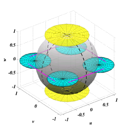
Figure 1: Bloch sphere (shaded shell) and coherent states of $SU(2)$. Dashed black curves mark intelligent coherent states. Ellipses denote $\Delta J_{x}$ and $\Delta J_{y}$ variance for ten coherent states: the atomic and molecular vacuum states (yellow), four non-intelligent states (cyan) and the four squeezed, minimum uncertainty states (magenta).

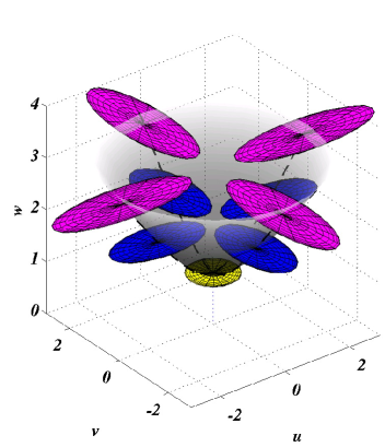
Figure 2: Surface of motion of $\langle{\bf K}\rangle=(u,v,w)$ (shaded paraboloid) and coherent states of $SU(1,1)$. Dashed black curves mark intelligent coherent states. Ellipses denote the $\Delta K_{x}$ and $\Delta K_{y}$ variances for nine intelligent coherent states. Whereas the atomic vacuum (yellow ellipse) is a minimum uncertainty state with equal variance in the ${\cal K}_{x}$ and ${\cal K}_{y}$ directions, other intelligent states (magenta,blue) are squeezed.

III.2 SU(1,1) Coherent states

The mutual eigenstates of the $SU(1,1)$ Casimir operator (29) and of $K_{z}$ form the basis set:

$$\left[K_{z}^{2}-K_{x}^{2}-K_{y}^{2}\right]|k,n\rangle=k(k-1)|k,n\rangle,$$ (49)

$$K_{z}|k,n\rangle=(k+n)|k,n\rangle,$$ (50)

with $n=0,1,\dots,N/2$. In analogy to Eq. (37), $SU(1,1)$ coherent states are obtained as

$$|\theta,\phi\rangle\equiv\exp\left(\beta K_{+}-\beta^{*}K_{-}\right)|k,0\rangle~{},$$ (51)

with $\beta=-(\theta/2)\exp(-i\phi)$ Barut . Power-series expansion of the exponents in Eq. (51) gives the $SU(1,1)$ coherent states in terms of the number states $|k,n\rangle$,

$$|\theta,\phi\rangle=\left[1-\tanh^{2}\left({\theta\over 2}\right)\right]^{k}\sum_{n=0}^{N/2}\left[-\tanh\left({\theta\over 2}\right)\exp(-i\phi)\right]^{n}\left(\frac{\Gamma(n+2k)}{n!\Gamma(2k)}\right)^{1/2}|k,n\rangle~{}.$$ (52)

Consequently, the expectation values of $\bf K$ are

$$\langle K_{x}\rangle = k\sinh\theta\cos\phi,$$ (53)

$$\langle K_{y}\rangle = k\sinh\theta\sin\phi,$$ (54)

$$\langle K_{z}\rangle = k\cosh\theta,$$ (55)

so that the motion of the vector $\langle{\bf K}\rangle$ is restricted to the paraboloid $\langle K_{z}\rangle^{2}-\langle K_{x}\rangle^{2}-\langle K_{y}\rangle^{2}=k^{2}$ (see Fig.2), as could be expected from the $SU(1,1)$ Casimir in Eq. (29). The variance of the $SU(1,1)$ generators for the coherent states (52) are given by

$$\Delta K_{x}^{2} = {M\over 2}\left(1+\sinh^{2}\theta\cos^{2}\phi\right)~{},$$ (56)

$$\Delta K_{y}^{2} = {M\over 2}\left(1+\sinh^{2}\theta\sin^{2}\phi\right)~{},$$ (57)

$$\Delta K_{z}^{2} = {M\over 2}\sinh^{2}\theta~{}.$$ (58)

Due to the possibility of multiple occupation in any single mode, neither the expectation values nor the variance of the $\bf K$ operators are bound. Since the structure constants of the two algebras differ only in sign, the uncertainty relations of $SU(1,1)$ are the same as for $SU(2)$, e.g.,

$$\Delta K_{x}\Delta K_{y}\geq{1\over 2}|\langle K_{z}\rangle|,$$ (59)

and we can define intelligent and minimum-uncertainty states as we did for $SU(2)$ in the previous subsection.In Fig 2 we plot the expectation values of $\bf K$ for $SU(2)$ coherent states, as well as the $\Delta K_{x}$ and $\Delta K_{y}$ variance of nine such states. It is clear from Eqs. (56),(57), and (55) that the intelligent states will be obtained for $\phi=0,\pi/2,\pi,3\pi/2$ and arbitrary $\theta$.

III.3 Generalized Squeezing

As is clear from Eqs. (48) and (59), the minimum fluctuation product of these two observables, depends on the expectation value of the remaining generator:

$$\Delta X_{i}^{2}\leq{1\over 2}|c_{ij}^{k}\langle{\hat{X}}_{k}\rangle|, ~{}{\rm and}~{} \Delta X_{j}^{2}\geq{1\over 2}|c_{ij}^{k}\langle{\hat{X}}_{k}\rangle|.$$ (60)

Generalized squeezed states of Lie algebras generated by $\{{\hat{X}}_{i}\}_{i=1,2,3}$ are defined as those states for which the variance in one observable has been reduced at the expense of another Wodkiewicz85 .

It is clear from Eqs. (41)-(46) that starting from a fermionic atomic vacuum and inducing a rotation about the $J_{x}$ axis (e.g., by choosing $\Delta=0$ and $g=g^{*}$), the variance in $J_{y}$ will be squeezed at the expense of $J_{x}$ fluctuations (see Fig. 1) because $1-\sin^{2}\theta\leq|\cos\theta|$ for all $\theta$. Similarly, rotating about the $J_{y}$ axis (e.g., by choosing $\Delta=0$ and $g=-g^{*}$) will result in generalized squeezing of $\Delta J_{x}$. The same is also true for rotations of a boson atomic vacuum, as seen from Eqs. (53)-(58). However, the way to attain generalized squeezing for fermions and bosons is quite different. Whereas with fermion atoms, squeezing in $J_{x}$ is obtained by reduction of its fluctuations, keeping a fixed $J_{y}$ variance (thereby reducing the product $\Delta J_{x}\Delta J_{y}=|J_{z}|/2$), the same goal is attained for boson atoms by increasing the variance of $K_{y}$ (thereby increasing $\Delta K_{x}\Delta K_{y}=|K_{z}|/2$)and keeping $K_{x}$ fluctuations fixed.

IV Short Time Dynamics

Since the atomic vacuum state (yellow disk in Figs. 1 and 2) is a coherent state, the atomic states produced in the dissociation of a molecular BEC will initially be coherent states of $SU(1,1)$ if the constituent atoms are bosons or of $SU(2)$ when the constituent atoms are fermions. There should thus be a significant difference in the short-time dynamics and in the initial fluctuations between the two cases. For bosons, one expects exponential amplification of atom-number and atom number fluctuations, whereas fermion number growth is more moderate and fluctuations remain bound. Physically, the source of these differences is in the underlying mechanisms of Bose-stimulation of dissociating boson pairs, leading to the dynamical instability of the atomic vacuum, and Pauli blocking of dissociating fermion pairs.

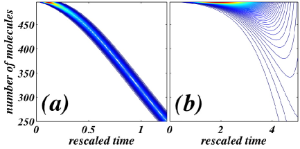
Figure 3: (color online) Number distributions as a function of rescaled time in the dissociation of $500$ molecules into fermion (a) and boson (b) constituent atoms.

In order to verify the formation of such coherent states and generalized squeezing, we have carried out many-particle simulations of molecular BEC dissociation into either fermionic or bosonic constituent atoms. For sufficiently short propagation times the molecular field is to a good approximation undepleted, and the generalized operators ${\cal J}_{i},{\cal K}_{i}$ coincide, up to an insignificant $c$-number, with the $SU$ generators $J_{i},K_{i}$. The atomic states during the initial stage of dissociation are thus approximately $SU(2)$ and $SU(1,1)$ coherent states respectively for fermion and boson constituents. In what follows, we shall numerically investigate to what extent do the generalized coherent states and squeezed fluctuations depicted in section III for an undepleted pump approximation, carry through to the operators ${\cal J}_{i},{\cal K}_{i}$, which account for pump depletion and fluctuations. In Fig. 3, we plot the atom-number distribution as a function of the rescaled time $\tau=g\sqrt{N}t$. The dissociation into fermion constituents shown in Fig. 3a, exhibits a Poissonian atom-number distribution with bound fluctuations as expected from Eqs. (43) and (46). Dissociation into boson constituents however, results in a super-Poissonian number distribution with an exponential growth of fluctuations as predicted in (55) and (58).

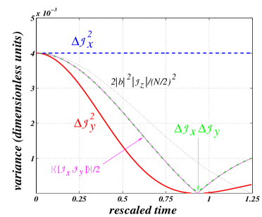
Figure 4: (color online) Quadrature variances $\Delta{\cal J}_{x}^{2}$ (dashed blue line), $\Delta{\cal J}_{y}^{2}$ (solid red line), and $\Delta{\cal J}_{x}\Delta{\cal J}_{y}$ (dash-dotted green line) as a function of the rescaled time $g\sqrt{N}t$, in the dissociation of a molecular BEC made of fermion-dimers. Pump phase is $\varphi=0$. The solid magenta line denotes the uncertainty limit $|\langle\left[{\cal J}_{x},{\cal J}_{y}\right]\rangle|/2$ which can be approximated at early times to be $2|b|^{2}|{\cal J}_{z}|/(N/2)^{2}$ (dotted black curve).

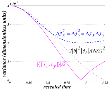
Figure 5: (color online) Same as Fig. 3, with pump phase $\varphi=\pi/4$. Quadrature variances $\Delta{\cal J}_{x}^{2}$, $\Delta{\cal J}_{y}^{2}$, $\Delta{\cal J}_{x}\Delta{\cal J}_{y}$ are all equal and greater than the uncertainty limit $|\langle\left[{\cal J}_{x},{\cal J}_{y}\right]\rangle|/2$ or its short-time approximation $2|b|^{2}|{\cal J}_{z}|/(N/2)^{2}$ (dotted black curve).

Generalized $SU(2)$ squeezing and its extension into the depleted-pump regime is illustrated in Fig. 4 and Fig. 5 where the variance in ${\cal J}_{x}$ and ${\cal J}_{y}$ in the dynamical evolution of the (fermion) atomic vacuum state, are plotted as a function of time. In Fig. 4, the phase of the association pump is $\varphi=0$, corresponding to rotation about the $u$ axis of the Bloch sphere of Fig. 1, i.e., $\phi=0$. The coalescence of the variance product $\Delta{\cal J}_{x}\Delta{\cal J}_{y}$ with the expectation value of the commutator $\langle[{\cal J}_{x},{\cal J}_{y}]\rangle$ demonstrates that the generated $SU(2)$ coherent state is indeed intelligent. Squeezing of the $\Delta{\cal J}_{y}$ variance while keeping a fixed $\Delta{\cal J}_{x}$ is observed, in agreement with the undepleted pump prediction. This reduction of ${\cal J}_{y}$ fluctuations eventually results in the expected minimum uncertainty state with $\Delta{\cal J}_{x}\Delta{\cal J}_{y}\approx 0$. In comparison, the evolution of variances for a $\varphi=\pi/4$ phase of the pump (corresponding to rotation along the $\phi=\pi/4$ circle on the Bloch sphere of Fig. 1) is shown in Fig. 5. The $SU(2)$ coherent states produced during this evolution, are non-intelligent, with equal $\Delta{\cal J}_{x}$ and $\Delta{\cal J}_{y}$ variances whose product is larger than the uncertainty limit.

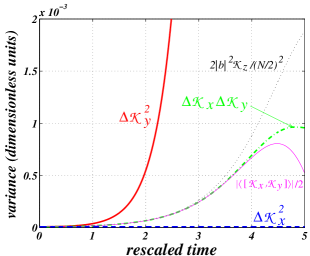
Figure 6: (color online) Quadrature variances $\Delta{\cal K}_{x}^{2}$ (dashed blue curve), $\Delta{\cal K}_{y}^{2}$ (solid red curve), and $\Delta{\cal K}_{x}\Delta{\cal K}_{y}$ (dash-dotted green curve) as a function of the rescaled time $g\sqrt{N}t$, in the dissociation of a molecular BEC made of boson-dimers. Pump phase is $\varphi=0$. The solid magenta curve denotes the uncertainty limit $|\langle\left[{\cal K}_{x},{\cal K}_{y}\right]\rangle|/2$ which coincides with $4|b|^{2}|{\cal K}_{z}|/(N/2)^{2}$ (dotted black curve) at early times where molecular depletion is negligible.

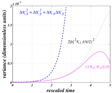
Figure 7: (color online) Same as Fig. 4, with pump phase $\varphi=\pi/4$. Quadrature variances $\Delta{\cal K}_{x}^{2}$, $\Delta{\cal K}_{y}^{2}$, $\Delta{\cal K}_{x}\Delta{\cal K}_{y}$ are all equal and greater than the uncertainty limit $|\langle\left[{\cal K}_{x},{\cal K}_{y}\right]\rangle|/2$ or its short-time approximation $2|b|^{2}|{\cal K}_{z}|/(N/2)^{2}$ (dotted black curve).

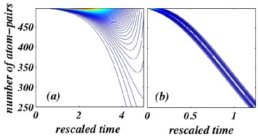
Figure 8: (color online) Number distributions as a function of rescaled time for the association of quantum degenerate gases of fermions (a) and bosons (b) with $N=1000$.

The time evolution of variances in the propagation of the atomic vacuum state for boson atoms, with $\varphi=0,\pi/4$, is shown respectively in Fig. 6 and Fig. 7. Unlike the fermion case where fluctuations are bound, we observed rapid increase in the $\Delta{\cal K}_{y}$ variance with a fixed $\Delta{\cal K}_{x}$, corresponding to motion on the $\phi=0$ parabola in Fig. 2. While the variance product $\Delta{\cal K}_{x}\Delta{\cal K}_{y}$ grows exponentially with time, its initial evolution traces the uncertainty limit $|\langle[{\cal K}_{x},{\cal K}_{y}]\rangle/2$ indicating that the produced states are indeed $SU(1,1)$ intelligent coherent states. Here too, propagation with a zero phase of the pump leads to the expected generalized squeezing. For $\varphi=\pi/4$ however, there is no squeezing as both $\Delta{\cal K}_{x}$ and $\Delta{\cal K}_{y}$ fluctuations are equal and exponentially growing. The $SU(1,1)$ coherent states produced are non-intelligent because the variance product $\Delta{\cal K}_{x}\Delta{\cal K}_{y}$ is larger than the uncertainty limit.

The agreement between the numerically-exact variance dynamics of Figs. 4-7 and the undepleted pump pictures of Fig. 1 and Fig. 2, demonstrates that the different collective dynamics predicted for fermion and boson constituent atoms can indeed be interpreted in terms of fluctuations of dynamical variables quadratic in the atomic creation or annihilation operators. The reduction of fluctuations of these variables is related to the formation of coherent states of the $SU(2)$ and $SU(1,1)$ Lie algebras. The same qualitative picture seems to apply to the depleted pump regime.

Finally, the mapping between fermion and boson dynamics, manifested in the equivalence of Eqs. (18)-(20) with $\eta=1$ and Eqs. (35) with $k=1/2$, is illustrated in Fig. 8 where atom number distributions are plotted as a function of time throughout the association of a Fermi (Fig. 8a) and Bose (Fig. 8b) atomic quantum gas. Fermion association is mapped onto boson dissociation (Fig. 3b) while boson association coincides with fermion dissociation (Fig. 3a), generating similar coherent states.

V Summary and Conclusions

We have established a connection between the collective behavior in boson and fermion pairing via Feshbach resonances and the generation of coherent states of the $SU(1,1)$ and $SU(2)$ Lie algebras. This relation provides a new viewpoint on the quantum statistics of atom-molecule quantum gas processes. The equivalence of molecular BEC dissociation with the Dicke model for fermion atoms Dicke54 and with parametric downconversion for boson atoms Walls_Milburn , known for some time in the quantum optics literature, is put into context as these two quantum systems are paradigmatic examples of the aforementioned algebras. The well known squeezing of fluctuations in dynamical variables linear in the atomic creation or annihilation operators (e.g. quadrature squeezing) during the dissociation into boson constituents, may be viewed as generalized $SU(1,1)$ squeezing of pair fluctuations, quadratic in the atomic creation and annihilation operators. Similarly, the coherent evolution during dissociation into fermion atoms corresponds to the generation of a minimum uncertainty $SU(2)$ coherent state. Our numerical simulations indicate that the same qualitative picture applies to the fluctuation of operators that account for molecular pump depletion. The presentation of the atom-molecule system in terms of these generators offers a link between the fermion- and boson-constituent atom cases due to the close relation and direct mapping between the underlying Lie algebras.

- (1) H. Feshbach, Ann. Phys. 19, 287 (1962); H. Feshbach, Theoretical Nuclear Physics, (Wiley, New York, NY, 1992).
- (2) S. Inouye, M. R. Andrews, J. Stenger, H.-J. Miesner, D. M. Staper-Kurn, and W. Ketterle, Nature (London) 392, 151 (1998).
- (3) C. A. Regal, C. Ticknor, J. L. Bohn, and D. S. Jin, Nature (London) 424, 47 (2003).
- (4) M. Greiner, C. A. Regal, and D. S. Jin, Nature (London) 426, 537 (2003).
- (5) S. Jochim, M. Bartenstein, A. Altmeyer, G. Hendl, S. Riedl, C. Chin, J. Hecker Denschlag, R. Grimm, Science 302, 2101 (2003).
- (6) M. W. Zwierlein, Z. Hadzibabic, S. Gupta, W. Ketterle, Phys. Rev. Lett. 91, 250401 (2003).
- (7) N. R. Claussen, E. A. Donley, S. T. Thompson, C. E. Wieman, Phys. Rev. Lett. 89, 010401 (2002).
- (8) J. Herbig, T. Krämer, M. Mark, T. Weber, C. Chin, H.-C. Nägerl and R. Grimm, Science 301, 1510 (2003).
- (9) S. Dürr, T. Volz, A. Marte and G Rempe, Phys. Rev. Lett. 92, 020406 (2004).
- (10) C. A. Regal, M. Greiner and D. S. Jin, Phys. Rev. Lett. 92, 040403 (2004).
- (11) M. W. Zwierlein, C. A. Stan, C. H. Schunck, S. M. F. Raupach, A. J. Kerman, W. Ketterle, Phys. Rev. Lett. 92, 120403 (2004).
- (12) M. Bartenstein, A. Altmeyer, S. Riedl, S. Jochim, C. Chin, J. Hecker Denschlag and R. Grimm, Phys. Rev. Lett. 92, 120401 (2004).
- (13) T. Bourdel, L. Khaykovich, J. Cubizolles, J. Zhang, F. Chevy, M. Teichmann, L. Tarruell, S. J. J. M. F. Kokkelmans and C. Salomon, Phys. Rev. Lett. 93, 050401 (2004).
- (14) J. Kinast, S. L. Hemmer, M. E. Gehm, A. Turlapov and J. E. Thomas, Phys. Rev. Lett. 92, 150402 (2004).
- (15) C. Chin, M. Bartenstein, A. Altmeyer S. Riedl S. Jochim, J. Hecker Denschlag, R. Grimm, Science 305, 1128 (2004).
- (16) M. Greiner, C. A. Regal and D. S. Jin, Phys. Rev. Lett. 94, 070403 (2005).
- (17) M. W. Zwierlein, C. H. Schunck, C. A. Stan, S. M. F. Raupach and W. Ketterle, Phys. Rev. Lett. 94, 180401 (2005).
- (18) T. Miyakawa and P. Meystre, Phys. Rev. A 71, 033624 (2005).
- (19) D. Meiser, P. Meystre and C. P. Search, Phys. Rev. A 71, 033621 (2005).
- (20) D. Meiser and P. Meystre, Phys. Rev. Lett. 94, 093001 (2005).
- (21) H. Uys, T. Miyakawa, D. Meiser and P. Meystre, Phys. Rev. A 72, 053616 (2005).
- (22) K. Wodkiewicz and J. H. Eberly, J. Opt. Soc. Am. B 2, 458 (1985).
- (23) A. V. Andreev, V. Gurarie and L. Radzihovsky, Phys. Rev. Lett. 93, 130402 (2004).
- (24) R. A. Barankov and L. S. Levitov, Phys. Rev. Lett. 93, 130403 (2004).
- (25) R. H. Dicke, Phys. Rev. 93, 99-110 (1954).
- (26) D.F. Walls and G.J. Milburn, Quantum Optics, (Springer- Verlag, 1995), Chapter 5; C. A. Holmes, G. J. Milburn. D. F. Walls, Phys. Rev. A39, 2493 (1989).
- (27) F. T. Arecchi, E. Courtens, R. Gilmore, and H. Thomas, Phys. Rev. A 6, 2211 (1972); A. M. Perelomov, Commun. Math. Phys. 26, 222 (1972); A. M. Perelomov, Usp. Fiz. Nauk 123, 23 (1977) [Sov. Phys. Usp. 20, 703 (1977)].
- (28) A. 0. Barut and R. Ra̧czka, Theory of Group Representation and Applications, (Polish Scientific Publishers, Warsaw, 1977).