First order transition in a three dimensional disordered system

Abstract

We present the first detailed numerical study in three dimensions of a first-order phase transition that remains first-order in the presence of quenched disorder (specifically, the ferromagnetic/paramagnetic transition of the site-diluted four states Potts model). A tricritical point, which lies surprisingly near to the pure-system limit and is studied by means of Finite-Size Scaling, separates the first-order and second-order parts of the critical line. This investigation has been made possible by a new definition of the disorder average that avoids the diverging-variance probability distributions that plague the standard approach. Entropy, rather than free energy, is the basic object in this approach that exploits a recently introduced microcanonical Monte Carlo method.

The combination of phase coexistence and chemical disorder plays a major role, for instance, in colossal magnetoresistance oxides MANGA . In these situations one faces a fairly general question: which are the effects of quenched disorder GIORGIO on systems that undergo a first-order phase transition in the ideal limit of a pure sample? For $D\!=\!3$ systems, $D$ being the space dimension, we only know that disorder somehow smoothes the transition. More is known in $D\!=\!2$, where the effects of disorder are so strong that the slightest concentration of impurities switches the transition from first-order to second-order Aize89 ; Card90 ; UNIVERSALIDAD2D .

An useful physical picture in $D\!=\!3$ is provided by the Cardy-Jacobsen conjecture Card90 . Consider a ferromagnetic system undergoing a first order phase transition for a pure sample. Let $T$ be the temperature while $p$ is the concentration of magnetic sites. A transition line, $T_{\mathrm{c}}(p)$ separates the ferromagnetic and the paramagnetic phases in the $(T,p)$ plane. In $D\!=\!3$ a critical concentration is expected to exist, $1>p_{\mathrm{t}}>0$, such that the phase transition is of the first-order for $p>p_{\mathrm{t}}$ and of the second order for $p<p_{\mathrm{t}}$ (at $p_{\mathrm{t}}$ one has a tricritical point). When $p$ approaches $p_{\mathrm{t}}$ from above, the latent-heat and the surface tension vanish while the correlation-length $\xi(T_{\mathrm{c}}(p))$ diverges. The Universality Class is expected to be related with that of the Random Field Ising Model (RFIM). However, the Cardy-Jacobsen conjecture relies on a mapping between two still unsolved models (in $D\!=\!3$), the (large $Q$) disordered Potts model WU and the RFIM.

Numerical simulation is an important tool for theoretical investigations in $D\!=\!3$. In this way, large portions of the transition line $T_{\mathrm{c}}(p)$ were found to be second order Ball00 ; Chat01 ; Chat05 . However, the study of the tricritical point as well as that of the first-order part of the transition line seemed hopeless. The problem comes from the long-tailed probability distribution functions (PDF) encountered at $T_{\mathrm{c}}(p)$, when comparing the specific-heat or the magnetic susceptibility of different samples Chat05 . Long tailed PDFs follows from the standard definition of the quenched free-energy at temperature $T$ as the average of the samples’ free-energy at the same $T$ GIORGIO , which is dominated by rare events . Furthermore, the simulation of a sample of linear size $L$ with previous methods is intrinsically hard even for a pure system (see NEUSHAGER ). In fact, previous work Chat01 ; Chat05 was limited to $L\leq 25$.

Here, we study for the first time the tricritical point separating the first and the second order pieces of the transition line. Furthermore, we characterize a first order transition that remains so in the presence of quenched disorder. This has been made possible by two alternative methods of performing the sample average that avoid long-tailed PDFs, reproduce the correct thermodynamic limit, and provide complementary information. Essential for this study has been the capability of studying directly the entropy, using a recently proposed microcanonical Monte Carlo method Mart07 combined with a cluster algorithm SW . We studied systems of size up to $L\!=\!128$, which allowed a neat Finite-Size Scaling investigation of the elusive tricritical point.

Specifically, we consider the site diluted $Q\!=\!4$ Potts model with periodic boundary conditions. The spins $\sigma_{i}\!=\!1,\ldots,Q$ occupy the nodes of a cubic lattice with probability $p$. We consider nearest neighbor interaction:

$${\cal H}^{\mathrm{spin}}=-\sum_{<i,j>}\epsilon_{i}\epsilon_{j}\delta_{\sigma_{i}\sigma_{j}}\,.$$ (1)

The $\epsilon_{i}$ are quenched occupation variables, ($\epsilon_{i}\!=\!0$ or 1 with probability $1-p$ and $p$ respectively) . The pure system, $p\!=\!1$, undergoes a first order phase transition Chat05 ; Mart07 which is generally regarded as very strong.

We introduce a real-valued conjugated momentum per occupied site, $\pi_{i}$ Mart07 . The total Hamiltonian is ${\cal H}\!=\!{\cal H}^{\mathrm{spin}}+\sum_{i}\epsilon_{i}\pi_{i}^{2}/2$ (the internal energy density will be $e\!=\!{\cal H}/N$ ). In the canonical ensemble, $\langle e\rangle_{T}\!=\!1/(2T)+\langle{\cal H}^{\mathrm{spin}}/N\rangle_{T}$. We consider instead the microcanonical ensemble for the extended model $\{\sigma_{i},\pi_{i}\}$ at fixed $e$, and integrate out the $\{\pi_{i}\}$ to obtain a Fluctuation-Dissipation formalism. The basic quantity is a function of $e$ and the spins, $\hat{\beta}\!=\!(N-2)/(Ne-{\cal H}^{\mathrm{spin}})\,$. Its microcanonical mean value $\beta_{\{\epsilon\}}(e)\!=\!\langle\hat{\beta}\rangle_{e}$ is the $e$-derivative of the entropy per spin, $s(e)$, for that particular sample $\{\epsilon\}$.

Connection with the canonical formalism is made by solving the equation $\beta_{\{\epsilon\}}(e)-1/T\!=\!0$, that yields the internal energy as a function of temperature. Thermodynamic stability requires $\beta_{\{\epsilon\}}(e)$ to be a decreasing function of $e$. Yet, at phase coexistence and for finite $N$, it is not (see Fig. 1 and Ref. Mart07 ): the equation $\beta_{\{\epsilon\}}(e)-1/T\!=\!0$ has several roots. For $T=T_{\mathrm{c}}$, we name respectively $e_{\mathrm{d}}$ and $e_{\mathrm{o}}$ the rightmost and leftmost solutions, that correspond to the energy densities of the coexisting disordered and ordered phases. The critical temperature is fixed by Maxwell construction: the $e$-integral of $\beta_{\{\epsilon\}}(e)-1/T_{\mathrm{c}}$ from $e_{\mathrm{d}}$ to $e_{\mathrm{o}}$ vanishes . The surface-tension, $\Sigma$, is $L^{D-1}/2$ times the integral of the positive part of $\beta_{\{\epsilon\}}(e)-1/T_{\mathrm{c}}$ for $e_{\mathrm{o}}<e<e_{\mathrm{d}}$.

For a disordered system, one analyzes the set of functions $\beta_{\{\epsilon\}}(e)$ corresponding to a large enough number of samples. There are two natural possibilities. On one hand, one can use the Maxwell construction for each sample, extracting $T_{\mathrm{c}}$, $e_{\mathrm{d}}$, $e_{\mathrm{o}}$ and $\Sigma$ and considering afterwards their sample average or even their PDF, Fig. 2. The second alternative is to compute the sample-average $\beta(e)=\overline{\beta_{\{\epsilon\}}(e)}$, and then perform on it the Maxwell construction (i.e. take the sample average of $s(e)$, rather than the average of the free-energy at fixed $T$).

We have empirically found that the two sample-averaging are equivalent in the first-order piece of the critical line. This is hardly surprising, because the internal energy as a function of $T$ is a self-averaging quantity for all temperatures but the critical one. Therefore, also $e_{\mathrm{d}}$, $e_{\mathrm{o}}$ and $T_{\mathrm{c}}$ are self-averaging properties in the first-order piece of the critical line. The first method offers more information but it is computationally more demanding (it requires high accuracy for each sample). The method featuring $\beta(e)$ can be used as well in the second-order part of the critical line, nevertheless its merit in that region are yet to be researched.

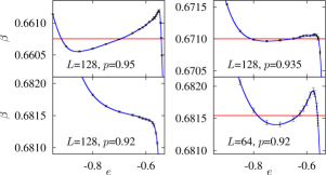
Figure 1: (color online). Sample-averaged $e$-derivative of the entropy, $\beta(e)$, for several lattice sizes, $L$, and spins concentrations, $p$. Metastability requires a non-decreasing $\beta(e)$. The horizontal line marks the critical (inverse) temperature $1/T_{\mathrm{c}}$, obtained through Maxwell’s construction. At fixed $L$ the surface tension increases for growing $p$. Note that, for fixed dilution, a seemingly first order transition ($L=64$, bottom-right), may actually be of the second order if studied on larger lattices ($L=128$, bottom-left).

We have investigated the phase transition for several $p$ values in the range $0.75\leq p\leq 1$. As a rule, we found that at fixed $p$ the latent heat is a monotonically decreasing function of $L$, Fig. 3. For each $p$ value, we simulated $L=16$, $32$, $64$ and $128$ (for a given $p$, we did not consider larger lattices once the latent heat vanished). For all pairs ($L$,$p$) we simulated 128 samples. Besides, some intermediate $L$ values were added for the Finite Size Scaling study below (see Fig. 4), and we have raised to 512 the number of samples for ($L=16,32$,  $p=0.86,0.875$).

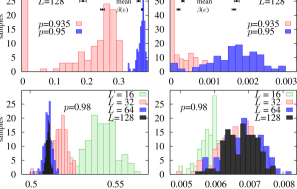
Figure 2: (color online). Histograms for the sample-dependent latent-heat $\upDelta_{\{\epsilon\}}e=e_{\mathrm{d}}-e_{\mathrm{o}}$ (left) and surface-tension (right). In the top panels we show results in the largest lattice, where two very close spin concentrations behaves very differently. The three types of drawn horizontal lines (indicating central value and statistical error) correspond, from top to bottom, to the median, the mean and the value obtained from $\beta(e)$. In the lower panels we show the histograms for $p=0.98$ and several $L$ (mind the difference in the horizontal scales with the upper part). The latent-heat is self-averaging while the surface tension is not.

We used a Swendsen-Wang (SW) version of the microcanonical cluster method Mart07 . For disordered systems, SW updates properly loosely connected regions ISDIL and does not require painful parameter tunings. For each sample, we simulated at least 20 $e$ values in the range $-1.2<e<-0.5$. The values of $e$ were decreased sequentially, to make use of the thermalization effort at the previous energy density. The microcanonical cluster method, which is not rejection-free, depends on a tunable parameter, $\kappa$. In order to maximize the acceptance of the SW attempt (SWA), $\kappa$ should be chosen as close as possible to $\beta_{\{\epsilon\}}(e)$. After every $e$ change, we performed cycles consisting of $10^{3}$ Metropolis steps, $\kappa$ refreshing, then $10^{3}$ SWA, and a new $\kappa$ refreshing. The cycling was stopped, and $\kappa$ fixed, when the SWA acceptance exceeded $60\%$. Afterwards we performed 2—$4\times 10^{5}$ SWA, taking measurements every 2 SWA. In addition, we performed thermalization checks that included comparisons of hot and cold starts or even mixed configurations (bandsMart07 ).

Our results for the latent-heat, $\upDelta e=e_{\mathrm{d}}-e_{\mathrm{o}}$, and the surface tension are in Fig. 3. The apparent location of the tricritical point (i.e. the $p$ where both $\upDelta e$ and $\Sigma$ vanish) shifts to upper $p$ for growing $L$ rather fast. For lattice sizes comparable with those of previous work, $L=16$, we obtain $p_{\mathrm{t}}^{L=16}\approx 0.75$, at a sizeable distance from $p\!=\!1$, but the estimate of $p_{\mathrm{t}}$ increases very fast with $L$.

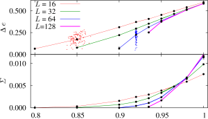
Figure 3: (color online). Top: Latent heat as obtained from $\beta(e)$ vs. spins concentration for several lattice sizes (lines are linear interpolations). Data for $p=1$ and $L\!=\!128$ were taken from Ref. Mart07 . To illustrate the sample dispersion, we plot as well the scatter-plot of ($N/L^{D}$, $\upDelta_{\{\epsilon\}}e$) for the 128 samples at $L\!=\!16$ $p\!=\!0.85$ and $L\!=\!64$ $p\!=\!0.92$. Bottom: as top part, for the surface tension.

The PDFs for $\upDelta e$ and $\Sigma$, Fig. 2, display an interesting $L$ evolution. When the $\beta(e)$ changes behavior from non-monotonic ($L=64$, Fig. 1, bottom-right) to monotonic ($L=128$, Fig. 1, bottom-left), the two PDFs becomes enormously wide, see top panels in Fig 2. This arises because for many $L=128$ samples, the curve $\beta_{\{\epsilon\}}(e)$ is becoming flat, or even monotonically decreasing (i.e. $\upDelta e\!=\!\Sigma=0$), while no such behavior was seen for $L\!=\!64$. Only for $p\!=\!0.98$, the width of the PDFs for $\upDelta e$ scales as $L^{-D/2}$, as expected for a self-averaging quantity, Fig. 2–bottom-left. The surface-tension is not self-averaging, Fig. 2–bottom-right.

From Figs. 1, 2 and 3 one cannot rule out that $p_{\mathrm{t}}=1$: a disordered first-order transition would not exist. Fortunately we can solve this dilemma by considering the correlation-length, obtained from the sample-averaged correlation function,

$$C(r)=L^{-D}\overline{\sum_{x}\epsilon_{x}\epsilon_{x+r}\left\langle\delta_{\sigma_{x},\sigma_{x+r}}-Q^{-1}\right\rangle_{e}}\ ,$$ (2)

as $\xi^{2}(e)=[-1+\widehat{C}(0,0,0)/\widehat{C}(2\pi/L,0,0)]/[2\sin\pi/L]$, where $\widehat{C}$ is the Fourier transform of $C(r)$  COOPER ; AMIT .

We take the correlation-length in units of the lattice size at $e_{\mathrm{d}},e_{\mathrm{o}}$ as obtained from $\beta(e)$ (a jackknife method AMIT takes care of the statistical correlations). For all $p<p_{\mathrm{t}}$, one expects that both $\xi(e_{\mathrm{d}})/L$ and $\xi(e_{\mathrm{o}})/L$ tend to non-vanishing and different limits for large $L$. On the other hand, for $p>p_{\mathrm{t}}$, $\xi(e_{\mathrm{d}})/L$ is of order $1/L$, while $\xi(e_{\mathrm{o}})/L\sim L^{D/2}$. For a fixed $L$, upon increasing $p$, the behavior goes from second-order like to first-order (see Fig 1). Hence, a Finite-Size Scaling approach AMIT is needed.

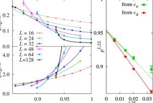
Figure 4: (color online). Left: Correlation length in units of the lattice size, at phase-coexistence for the paramagnetic (top) and ordered (bottom) phases , as a function of spin concentration for several $L$ (lines are cubic spline interpolations for data at fixed $L$). Right: Spin concentration where $\xi/L$ (data from left panel) coincide for lattices $L$ and $2L$ versus $1/L^{x}$, see Eqs.(3,4). Lines are a joint fit for $x$, $p_{\mathrm{t}}$, $A_{\mathrm{d}}$ and $A_{\mathrm{o}}$.

Consider the curves of $\xi(e_{\mathrm{d}})/L$ versus $p$, for different $L$, Fig. 4 (left-top). There is a unique concentration, $p^{L,2L}$, where the correlation length in units of the lattice size coincides for lattices $L$ and $2L$. One has 

$$p^{L,2L}\approx p_{\mathrm{t}}+A_{\mathrm{d}}L^{-x}\,,$$ (3)

An analogous result holds for $\xi(e_{\mathrm{o}})/L$. Since $A_{\mathrm{d}}$ and $A_{\mathrm{o}}$ are rather different, see Fig. 4—right, a joint fit of all data yields an accurate estimate for the location of the tricritical point:

$$p_{\mathrm{t}}=0.954(3),\ x=1.23(9),\ \frac{\chi^{2}}{\mathrm{dof}}=\frac{4.23}{3}\,,$$ (4)

Of course, due to higher-order scaling corrections, Eq.(3) should be used only for lattices larger than some $L^{\mathrm{min}}$ ON-RP2 . The fit $\chi^{2}$ was acceptable taking $L^{\mathrm{min}}_{\mathrm{o}}=16$ and $L^{\mathrm{min}}_{\mathrm{d}}=12$ (for the sake of clarity we do not display data for $L=12$ in the figures). We thus conclude that $p=0.98$ is definitively in the first-order part of the critical line.

We now look at $\xi/L$ at $p^{L,2L}$, Fig 4. Consider $\xi(e_{\mathrm{d}})/L$ ($\xi(e_{\mathrm{o}})/L$) as a function of $(L,p)$, in the region $p<p_{\mathrm{t}}$. The salient features are: (i) for fixed $L$, $\xi(e_{\mathrm{d}})/L$ is a decreasing function of $p$ ($\xi(e_{\mathrm{o}})/L$ is increasing); (ii) for fixed $p$, $\xi(e_{\mathrm{d}})/L$ has a minimum ($\xi(e_{\mathrm{o}})/L$ has a maximum), at a crossover length scale, $L_{\mathrm{co}}(p)$, that separates the first-order like behavior from the second order one; (iii) at the crossing point $p^{L,2L}$ we have $L<L_{\mathrm{co}}(p^{L,2L})<2L$; (iv) at least within the range of our simulations, $L_{\mathrm{co}}(p)$ is a growing function of $p$. A standard scaling argument, combined with (i)—(iv), yields that $\xi(e_{\mathrm{d}})/L$ at $p^{L,2L}$ is of order $1/L_{\mathrm{co}}$ ($\xi(e_{\mathrm{o}})/L\sim L^{D/2}_{\mathrm{co}}$). If $L_{\mathrm{co}}(p)$ diverges at $p_{\mathrm{t}}$, $\xi(e_{\mathrm{d}})/L$ at $p^{L,2L}$ should tend to zero for large $L$, which is indeed consistent with our data.

In this work, we have performed for the first time a detailed study of a disordered first-order transition in $D\!=\!3$, by site-diluting the $Q\!=\!4$ Potts model, a system suffering a prototypically strong first-order transition. A fairly small degree of dilution smooths the transition to the point of becoming second order, at a tricritical point, $p_{\mathrm{t}}$. A delicate Finite-Size Scaling analysis is needed to firmly conclude that $p_{\mathrm{t}}<1$. We thus claim that (quenched) disordered first-order transitions do exist in $D\!=\!3$, although quenched disorder is astonishing effective in smoothing the transition (we speculate that the percolative mechanism for colossal magnetoresistance proposed in MANGA could be fairly common in $D\!=\!3$). We also observe that, for a given $p<p_{\mathrm{t}}$, a crossover length scale $L_{\mathrm{co}}(p)$ exists such that for $L<L_{\mathrm{co}}(p)$ the behavior is first order like. The asymptotic second-order behavior appears only for $L>L_{\mathrm{co}}(p)$. Our data are consistent with a divergence of $L_{\mathrm{co}}(p)$ at $p_{\mathrm{t}}$. The successful location of the tricritical point has been made possible by new definitions of the quenched average that avoids long-tailed PDF Chat05 . It was crucial in this approach a recently introduced microcanonical Monte Carlo method that features the entropy density rather than the free energy Mart07 .

This work has been partially supported by MEC through contracts No. FIS2004-01399, FIS2006-08533-C03, FIS2007-60977 and by CAM and BSCH. Computer time was obtained at BIFI, UCM, UEX and, mainly, in the Mare Nostrum. The authors thankfully acknowledge the computer resources and technical expertise provided by the Barcelona Supercomputing Center.

References

- (1) E. Dagotto, Science 309, 258 (2005); J. Burgy et al., Phys. Rev. Lett. 87, 277202 (2001); ibid 92, 097202 (2004); C. Sen, G. Alvarez and E. Dagotto, Phys. Rev. Lett. 98, 127202 (2007).
- (2) See e.g. G. Parisi Field Theory, Disorder and Simulations. World Scientific 1994.
- (3) M. Aizenman and J. Wehr, Phys. Rev. Lett. 62, 2503 (1989); K. Hui and A.N. Berker ibid 62, 2507 (1989).
- (4) J. Cardy and J.L. Jacobsen, Phys. Rev. Lett. 79, 4063 (1997); Nucl. Phys. B, 515, 701 (1998).
- (5) C. Chatelain and B. Berche, Phys. Rev. Lett. 80, 1670 (1998); Phys. Rev E 58, R6899 (1998); ibid 60, 3853 (1999).
- (6) F.Y. Wu, Rev. Mod. Phys. 54, 235 (1982).
- (7) C. Chatelain, B. Berche, W. Janke, and P.-E. Berche, Phys. Rev. E 64, 036120 (2001).
- (8) C. Chatelain, B. Berche, W. Janke, and P.-E. Berche, Nucl. Phys. B 719, 275 (2005).
- (9) H. G. Ballesteros, L. A. Fernández, V. Martin-Mayor, A. Muñoz Sudupe, G. Parisi and J. J. Ruiz-Lorenzo. Phys. Rev. B 61, 3215 (2000).
- (10) M.S.S. Challa, D.P. Landau, and K. Binder, Phys. Rev. B 34, 1841 (1986); J. Lee and J.M. Kosterlitz, Phys. Rev. Lett. 65, 137 (1990).
- (11) J.T. Chayes, L. Chayes, D.S. Fischer and T. Spencer, Phys. Rev. Lett. 57, 2999 (1986); A. Maiorano, V. Martin-Mayor, J.J. Ruiz-Lorenzo and A. Tarancon, Phys. Rev. B 76, 064435 (2007).
- (12) T. Nehaus and J.S. Hager, J. of Stat. Phys. 113, 47 (2003).
- (13) V. Martin-Mayor, Phys. Rev. Lett. 98, 137207 (2007).
- (14) R.H. Swendsen and J.S. Wang, Phys. Rev. Lett. 58, 86 (1987).
- (15) D. Stauffer and A. Aharony in Introduction to the percolation theory. (Taylor and Francis, London 1984).
- (16) H.G. Ballesteros et al., Nucl. Phys. B 512, 681 (1998); Phys. Rev. B 58, 2740 (1998).
- (17) F. Cooper, B, Freedman and D. Preston, Nucl. Phys. 210, 210 (1982).
- (18) D. Amit and V. Martin-Mayor, Field Theory, the Renormalization Group, and Critical Phenomena, World-Scientific Singapore 2005.
- (19) H.G. Ballesteros, L.A. Fernandez, V. Martin-Mayor and A. Muñoz Sudupe, Phys. Lett, B 378, 207 (1996); ibid 387, 125 (1996).