FDTD Computation of Human Eye Exposure to Ultra-wideband Electromagnetic Pulses

Abstract

With an increase in the application of ultra-wideband (UWB) electromagnetic pulses in the communications industry, radar, biotechnology and medicine, comes an interest in UWB exposure safety standards. Despite an increase of the scientific research on bioeffects of exposure to non-ionizing UWB pulses, characterization of those effects is far from complete. A numerical computational approach, such as a finite-difference time domain (FDTD) method, is required to visualize and understand the complexity of broadband electromagnetic interactions. The FDTD method has almost no limits in the description of the geometrical and dispersive properties of the simulated material, it is numerically robust and appropriate for current computer technology. In this paper, a complete calculation of exposure of the human eye to UWB electromagnetic pulses in the frequency range of 3.1-10.6, 22-29, and 57-64 GHz is performed. Computation in this frequency range required a geometrical resolution of the eye of $\rm 0.1\>mm$ and an arbitrary precision in the description of its dielectric properties in terms of the Debye model. New results show that the interaction of UWB pulses with the eye tissues exhibits the same properties as the interaction of the continuous electromagnetic waves (CW) with the frequencies from the pulse’s frequency spectrum. It is also shown that under the same exposure conditions the exposure to UWB pulses is from one to many orders of magnitude safer than the exposure to CW.

1 Introduction

While a large number of experiments have been performed in an attempt to provide an insight into the biological effects of the electromagnetic fields (Barnes and Greenebaum 2006, Miller et al 2002, Polk and Postow 1995), the bioeffects of non-ionizing ultra-wideband (UWB) electromagnetic (EM) pulses have not been studied in as much detail as the effects of continuous-wave (CW) radiation. Nevertheless, as the interest for the application of UWB electromagnetic pulses increases, particularly in the communications industry and medicine, so does the interest to understand their bioeffects (Zastrow et al 2007, Ji et al 2006, Hu et al 2005, Schoenbach et al 2004). Only recently was the work in the UWB field in the United States declassified (Taylor 1995), and only in 2002 were UWB pulses approved by the Federal Communications Commission in the U.S. for “applications such as radar imaging of objects buried under the ground or behind walls and short-range, high-speed data transmissions” (FCC 2002).

A computational approach to the exposure of biological tissues to non-ionizing UWB radiation is more involved than the computation of exposure to CW radiation. In addition to a realistic description of the geometry, the physical properties of exposed biological material have to be known over a broad frequency range. The computation has to be numerically robust and appropriate for the computer technology of today. The finite difference-time domain (FDTD) method, introduced by Kane Yee in the 1960s (Yee 1966) and extensively developed in the 1990s (Sadiku 1992, Kunz and Luebbers 1993, Sullivan 2000, Taflove and Hagness 2000), is a well known numerical method that satisfies these conditions.

The response of a biological system to an EM pulse relates to the extent of conversion of EM pulse energy into mechanical or thermal energy as the pulse propagates through the material. Calculating the electric and magnetic fields around and inside the exposed material and combining these with the electromagnetic properties of the exposed material, the specific absorption rate, total deposited energy, and induced current inside the sample can be calculated. Finally, the interaction mechanism between the electromagnetic radiation and biological material can be modeled and understood. It is possible that the bioeffects of short EM pulses are qualitatively different from those of narrow-band radio frequencies. If, for example, the specific absorption rate standards defined for continuous radio frequency by the American National Standard Institute (ANSI 1992) or by the International Commission on Non-Ionizing Radiation Protection (ICNIRP 1998) are applied to the short UWB pulses, their meaning loses its clarity. Because of the pulses’ short duration and as a result of the non-uniform power absorption, the deposition power and the induced current densities are large and can exceed locally even the highest allowed power limit of 4 W/kg (Simicevic 2007). At the same time, the energy from the exposure to an UWB pulse is too small to induce an increase in the temperature of the exposed sample due to, compared to CW, the much lower energy density of the UWB pulse.

We have already applied the FDTD method to calculate the EM fields inside biological samples exposed to nanopulses in a GTEM cell (Simicevic and Haynie 2005, Simicevic 2005). We included in the calculation the geometry and the physical properties of the samples to the fullest extent and applied a full three-dimensional computation, but have restricted the calculation to one sample (blood) and the frequency range up to $\rm 15\;GHz$.

In this paper, the effects of the exposure of a human eye to UWB radiation in the frequency range of up to $\rm 90\;GHz$ are calculated using the same three-dimensional FDTD computer code described and validated in the previous works (Simicevic and Haynie 2005, Simicevic 2005). The shape and the physical properties of the eye are described as accurately as allowed by the existing data. The computational space of $\rm 30\;mm$ $\times$ $\rm 26\;mm$ $\times$ $\rm 26\;mm$ was divided into $\rm\sim 2.0\times 10^{7}$ cells and the computation was performed at the Louisiana Optical Initiative (LONI) cluster of supercomputers. The eye was exposed to the UWB pulses from three different frequency regions: $\rm 3.1-10.6\;GHz$ (authorized for communications and radar imaging), $\rm 22-29\;GHz$ (authorized for vehicle radars), and $\rm 57-64\;GHz$ (authorized for unlicensed use) (FCC 2002).

What follows is a detailed description of the computation: geometrical and physical properties of the eye, the properties of the UWB pulses, the details of the computation and data representation, and the results.

2 The Shape and the Size of a Human Eye

The shape and the size of a human eye, an example of which is shown in Figure 1, varies from one individual to another and changes with age. While the theoretical eye models put the emphasis mostly on the optical properties of the eye (Norrby et al 2007, de AlmeidaI and Carvalho 2007, Siedlecki et al 2004, Lotmar 1971), they can as well be used in radiation protection (Charles and Brown 1975).

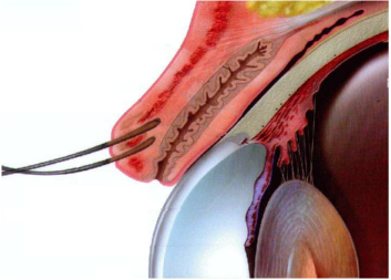
Figure 1: Schematics of the human eye.

For the application in the FDTD computing, the shape of the human eye was discretized by means of Yee cells, cubes of an edge length $\Delta x$ (Yee 1966). The two-dimensional shape of the eye shown in Figure 1 was normalized to the dimensions of the existing theoretical eye models, the pixels belonging to different eye tissues were retrieved by image processing software, and, because of rotational symmetry, rotation around the proper axis of rotation was performed to create the three dimensional model of the eye. To account for as small structures of the eye as, for example, the thickness of the cornea (only $\rm\sim 0.6-0.7\;mm$ in size), and still be able to perform the computation in a reasonable time, the lengths of the Yee cell were chosen to be $\rm\Delta x=\Delta y=\Delta z=0.1\;mm$ The computation was performed inside the computational space of $\rm 30\;mm$ $\times$ $\rm 26\;mm$ $\times$ $\rm 26\;mm$ in size discretized by $\rm\sim 2.0\times 10^{7}$ cells. The front part of the eye constructed from Yee cells is shown in Figure 2. To make Figure 2 readable, 16 Yee cells used in the computation are presented as one cell in the figure.

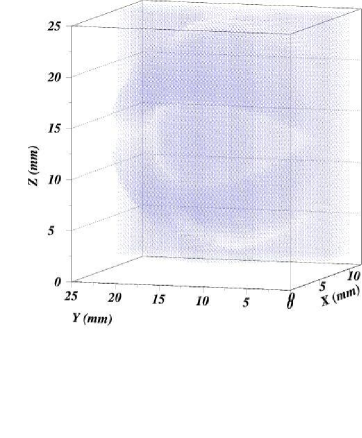
Figure 2: Front of the human eye discretized by means of Yee cells. One cell in the figure represents 16 Yee cells used in the computation.

During the process of discretization of the human eye, the structures of the eye were separated into the tissues of known dielectric properties: sclera, vitreous humour, lens cortex, cornea, lens nucleus, muscles, and blood. The eye was embedded in the bone, muscle and skin tissue (wet and dry). When dealing with UWB radiation it was crucial to have a proper description of the dielectric properties of the exposed tissues over the entire frequency range. They were taken from the established references (Gabriel 1996, Gabriel C et al 1996, Gabriel S et al 1996).

From the relation between the size of a Yee cell $\Delta x$ and the maximum frequency $f_{max}$ allowed in the FDTD computation (Kunz and Luebbers 1993, Taflove and Hagness 2000)

$$\Delta x\simeq{v\over{10\;f_{max}}},$$ (1)

where $v$ is the speed of light in the material, the Yee cube edge length of $\rm\Delta x=0.1\;mm$ may be used to model exposure to the wave frequency of up to $\rm 90\;GHz$. This value is far greater than the frequency range of the UWB pulses used in the calculation. We have achieved an optimal agreement between geometrical description of the eye and the computational requirements of the FDTD method.

3 Shape of the UWB Pulses

The eye was exposed to vertically polarized EM pulses, each covering one of three different frequency regions: $\rm 3.1-10.6\;GHz$, $\rm 22-29\;GHz$, and $\rm 57-64\;GHz$. The shape of the pulse is obtained by the inverse Fourier transformation of the uniform spectral density of frequency width $\rm\Delta f$ around the central frequency $\rm f_{c}$ of the frequency region. In the time domain, this transform is described by the function

$$E=E_{0}{\sin[\pi\Delta f(t-t_{0})]\over{\pi\Delta f(t-t_{0})}}\cos[2\pi f_{c}(t-t_{0})]e^{-{(t-t_{0})^{2}\over{2\sigma^{2}}}},$$ (2)

where $E_{0}$ is the pulse amplitude, $t_{0}$ is the time shift of the pulse, and $\rm\sigma$ is the pulse width. The exponential term $\rm e^{-{(t-t_{0})^{2}\over{2\sigma^{2}}}}$ allows for a smooth rise and fall of the pulse having, at the same time, a small effect on the pulse spectral density. The numerical value of the parameter $t_{0}$ was the same for all the frequency regions, $t_{0}=3\sigma$. For the frequency region of $\rm 3.1-10.6\;GHz$: $\rm\sigma=166.7\;ps$, $\rm\Delta f=7.5\;GHz$ and $\rm f_{c}=6.85\;GHz$, for the frequency region of $\rm 22-29\;GHz$: $\rm\sigma=66.7\;ps$, $\rm\Delta f=7\;GHz$ and $\rm f_{c}=25.5\;GHz$; and for the frequency region of $\rm 57-64\;GHz$: $\rm\sigma=66.7\;ps$, $\rm\Delta f=7\;GHz$ and $\rm f_{c}=60.5\;GHz$. The shapes and the frequency spectra of the pulses are plotted in Figure 3.

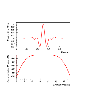
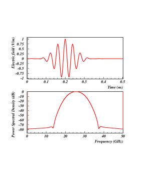
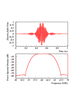
Figure 3: Shapes and frequency spectra of the UWB pulses described by Equation 2. The amplitudes are normalized to $\rm 1\;V/m$. From the left are the shape and the spectrum for the pulse in the frequency region of $\rm 3.1-10.6\;GHz$, pulse in the region of $\rm 22-29\;GHz$, and pulse in the region of $\rm 54-67\;GHz$.

Understanding the propagation of a UWB pulse is more demanding than understanding the propagation of a continuous EM wave. For some pulse frequencies the exposed sample looks like a conductor while for others it looks like a dielectric. The amount of the conduction currents compared to the displacement currents changes over the frequency spectrum of the EM pulse. In this paper we have restricted ourselves to studying the propagation of the pulses with almost uniform power spectra in the frequency range imposed by the FCC rules.

4 Dielectric Properties of the Exposed Eye Tissue

Electromagnetic properties of a tissue are normally expressed in terms of frequency-dependent dielectric properties and conductivity. When dealing with an UWB electromagnetic pulse, it is crucial that these properties are properly described over a large frequency range. One of the most accepted models describing the dielectric properties of a tissue is the Cole-Cole model. The references (Gabriel 1996, Gabriel C et al 1996, Gabriel S et al 1996)) provide the four-term Cole-Cole parametrization of the dielectric properties of the ocular tissue used in the present work

$$\varepsilon(\omega)=\varepsilon_{\infty}+\sum_{k=1}^{4}{\Delta\varepsilon_{k}\over{1+(i\omega\tau_{k})^{1-\alpha_{k}}}}+{\sigma\over i\omega\varepsilon_{0}}.$$ (3)

In this equation $i=\sqrt{-1}$, $\varepsilon_{\infty}$ is the permittivity in the terahertz frequency range, $\Delta\varepsilon_{k}$ are the changes in permittivity in a specified frequency range, $\tau_{k}$ are the relaxation times, $\sigma$ is the ionic conductivity, and $\alpha_{k}$ are the coefficients specific for the Cole-Cole model. They constitute up to 14 real parameters of a fitting procedure.

Application of the Cole-Cole model is problematic for FDTD. It requires time consuming numerical integration techniques and makes computation unacceptably slow. If, instead of a Cole-Cole parametrization, the Debye model

$$\varepsilon(\omega)=\varepsilon_{\infty}+\sum_{k=1}^{N}{\Delta\varepsilon_{k}\over{1+i\omega\tau_{k}}}+{\sigma\over i\omega\varepsilon_{0}}$$ (4)

is used, the computation time can be reduced by an order of magnitude using very efficient piecewise-linear recursive convolution (PLRC) method (Luebbers et al 1990, 1991, Luebbers and Hunsberger 1992, Kunz and Luebbers 1993, Taflove and Hagness 2000). But, it is also important that the Debye model provides an equally accurate description of the physical properties of a biological tissue.

In his thesis, G. R. Lugo (Lugo 2006) used an accurate, robust and efficient vector fitting technique (VECTFIT) (Gustavsen and Semlyen 1999) to replace the Cole-Cole parametrization by a multi-term Debye parametrization with no loss in the precision. His procedure is used in this paper. While the accuracy of the Debye parameterization increases with the number of terms, so does the computational time and the requirement on the memory, and an optimal number of terms has to be selected. It was found that in the frequency region considered in this paper the accuracy of the three-term Debye model

$$\varepsilon(\omega)=\varepsilon_{\infty}+{{\varepsilon_{s1}-\varepsilon_{\infty}}\over{1+i\omega\tau_{1}}}+{{\varepsilon_{s2}-\varepsilon_{\infty}}\over{1+i\omega\tau_{2}}}+{{\varepsilon_{s3}-\varepsilon_{\infty}}\over{1+i\omega\tau_{3}}}$$ (5)

is approximately the same as the accuracy of the corresponding Cole-Cole model. The parameters of the three-term Debye model for the tissue used in the calculation are presented in Table 1 and the comparison between the two models is shown in Figure 4.

Material	$\varepsilon_{\infty}$	$\varepsilon_{s1}$	$\varepsilon_{s2}$	$\varepsilon_{s3}$	$\tau_{1}(s)$	$\tau_{2}(s)$	$\tau_{3}(s)$	$\sigma(S/m)$
Blood	6.5	50.7	16.2	9835.	$7.95\;10^{-12}$	$4.08\;10^{-10}$	$7.35\;10^{-8}$	0.7
Bone Cortical	3.2	7.7	3.4	137.	$1.01\;10^{-11}$	$2.07\;10^{-10}$	$2.11\;10^{-8}$	0.02
Cornea	6.3	44.2	22.9	6122.	$7.73\;10^{-12}$	$4.75\;10^{-10}$	$5.59\;10^{-8}$	0.4
Lens Cortex	5.9	37.9	8.7	3873.	$7.57\;10^{-12}$	$3.33\;10^{-10}$	$5.96\;10^{-8}$	0.3
Lens Nucleus	4.3	29.1	9.9	996.	$8.34\;10^{-12}$	$4.33\;10^{-10}$	$3.24\;10^{-8}$	0.2
Muscle	6.5	45.2	11.9	5018.	$7.00\;10^{-12}$	$3.71\;10^{-10}$	$6.60\;10^{-8}$	0.2
Sclera	6.3	45.3	13.5	6912.	$7.61\;10^{-12}$	$3.86\;10^{-10}$	$7.07\;10^{-8}$	0.5
Skin Wet	5.9	36.0	21.1	1417.	$7.75\;10^{-12}$	$4.85\;10^{-10}$	$2.70\;10^{-8}$	0.0
Vitreous Humour	4.2	65.1	$3.6\;10^{7}$	-	$7.32\;10^{-12}$	$2.14\;10^{-4}$	-	1.5

Table 1: Debye parameters for the tissues used in the computation. Static conductivity $\sigma$ is from Reference (Gabriel C et al 1996).

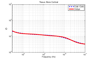
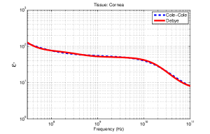
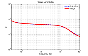
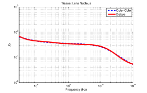
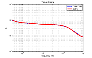
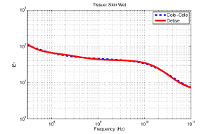
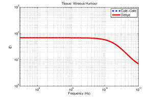
Figure 4: Comparison of the relative permittivity of the tissues used in the computation parametrized by the Debye model (Equation 5; red solid line) and the Cole-Cole model (Equation 3; blue dashed line). Parametrization covers frequency range from 30 MHz to 100 GHz.

5 Field Calculation and Data Representation

The quantities required to understanding the mechanisms and the consequences of the interaction between the electromagnetic radiation and biological tissue are obtained from the the values of electric and magnetic field components inside the tissue. Those components are accurate on the level of our knowledge of the physical properties of the exposed material. While the rapid developments in computer technology allow for the improvement of the geometrical description and for a longer exposure time calculation, for a reliable output, the knowledge of the physical properties of the material must be complete and correct. This is particularly important when simulating the interaction of UWB radiation with biological material.

A qualitative understanding of the penetration of an EM pulse into the eye can already be achieved from the animated sequences of the pulse propagation. For the case of the propagation of the UWB pulses used in this paper, the complete animation can be accessed on-line (Simicevic 2007). Only selected snapshots of the intensity of the pulse penetrating the eye, shown in Figures 5, 6, and 7, can be presented in this paper.

To understand the dosimetric implication from the exposure of a tissue to an electromagnetic pulse, or to model the interaction mechanism, a quantitative approach is needed. It mostly relates to the extent of conversion of EM pulse energy into mechanical or thermal energy inside the tissue. A detailed study is presented in the next section.

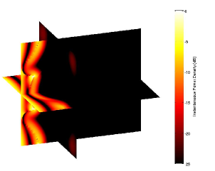
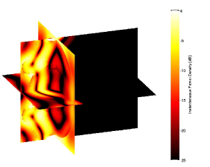
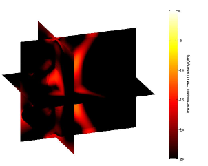
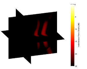
Figure 5: Four different stages of penetration of EM pulse, in the frequency region of $\rm 3.1-10.6\;GHz$, into the eye. The contours represent the instantaneous power density in decibels. Brighter regions correspond to higher power density.

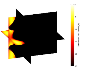
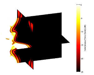
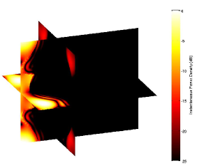
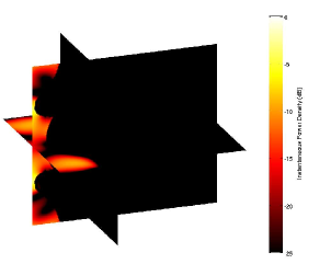
Figure 6: Four different stages of penetration of EM pulse, in the frequency region of $\rm 22-29\;GHz$, into the eye. The contours represent the instantaneous power density in decibels. Brighter regions correspond to higher power density.

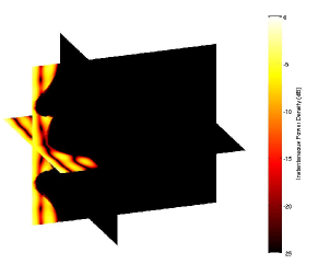
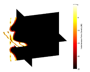
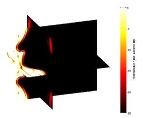
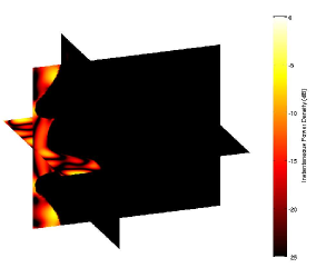
Figure 7: Four different stages of penetration of EM pulse, in the frequency region of $\rm 57-64\;GHz$, into the eye. The contours represent the instantaneous power density in decibels. Brighter regions correspond to higher power density.

6 Computation of Energy Dissipation for an Electromagnetic Pulse

If an electromagnetic pulse propagates through biological material, the energy will be dissipated inside the material. The conversion of electromagnetic energy into mechanical or thermal energy inside a volume $V$ is computed using equation (Jackson 1999)

$$P=\int_{V}\vec{J}\cdot\vec{E}\;dV.$$ (6)

$P$ is deposited energy per unit time, and $\vec{J}$ and $\vec{E}$ are, respectively, the current density and electric field inside the material. In the case of dispersive media, like the eye tissue, using Equation 6 is not trivial. First, the equation assumes a continuous distribution of charges and currents, which is not the case for the EM pulse propagation through tissue. Second, the current $\vec{J}$ consists of the conduction or ionic currents and of the displacement currents, which have to be correctly resolved (Jackson 1999).

To properly calculate the amount of the absorbed energy inside the eye tissue, one first eliminates the current $\vec{J}$ in Equation 6 using the Ampere-Maxwell law (Jackson 1999). The deposited energy per unit time is then expressed as a function of the EM fields inside the material

$$P=-\int_{V}\left[\vec{\nabla}\cdot(\vec{E}\times\vec{H})+\vec{E}\cdot{\partial\vec{D}\over\partial t}+\vec{H}\cdot{\partial\vec{B}\over\partial t}\right]\;dV.$$ (7)

$\vec{D}$ in this formula represents the electric displacement and $\vec{B}$ the magnetic induction. Volume integration covers the volume of the exposed object.

Equation 6 consists of the term $\vec{E}\times\vec{H}$, representing the energy flux density, and the term $\vec{E}\cdot{\partial\vec{D}\over\partial t}+\vec{H}\cdot{\partial\vec{B}\over\partial t}$, representing the total electromagnetic energy density. In the case of linear lossless non-dispersive media, the second term is interpreted as the difference of internal energy per unit volume with or without the presence of the EM field. In the case of linear dispersive media with losses, the case in this paper, such an interpretation is not trivial (Landau and Lifshitz 1960). In addition, the dispersion causes temporally non-local connection between $\vec{D}$ and $\vec{E}$

$$\vec{D}(\vec{r},t)=\varepsilon_{0}\varepsilon_{\infty}\vec{E}(\vec{r},t)+\varepsilon_{0}\int_{0}^{t}\chi(\tau)\vec{E}(\vec{r},t-\tau)\;d\tau.$$ (8)

Here $\varepsilon_{0}$ is permittivity of the free space, $\varepsilon_{\infty}$ the permittivity at infinite frequency, and $\chi(\tau)$ is the susceptibility (Fourier transform of complex relative permittivity). This makes a direct calculation of total internal electromagnetic energy very difficult.

In this paper, the dissipation of electromagnetic energy was calculated using the energy flux density. It was shown (Landau and Lifshitz 1960) that the formula for the energy flux density or Poynting vector $\vec{S}$

$$\vec{S}=\vec{E}\times\vec{H},$$ (9)

is valid for variable fields even if dispersion is present. It is obvious that the difference of the energy flux entering a volume $V$ and the flux exiting the same volume represents the amount of the energy dissipated inside the volume. In the case of UWB radiation, this energy is obtained by integrating the Poynting vector over the pulse duration $T$ and the impact area $\vec{A}$ enclosing the volume

$$E=\int_{T}\left[\oint_{A}\vec{S}\cdot d\vec{a}\right]dt.$$ (10)

Due to the absorption, this energy is ultimately converted into heat (Landau and Lifshitz 1960). As a basic volume of interest we have chosen the Yee cell and performed numerical integration of Equation 10 as

$$E=\sum_{Pulse\;duration}\left[\sum_{Yee\;cell\;area}\vec{S}\cdot\Delta\vec{a}\right]\Delta t.$$ (11)

$\Delta\vec{a}$ is an element of the Yee cell area and $\Delta t$ is the time step in the FDTD computation. Due to the offset in the location of the electric and magnetic field components relative to each other, and relative to the position of the Poynting vector, the value of the Poynting vector is obtained by using the average values of the adjacent field components. As an example, with the notation from Figure 8, the $S_{x}$ component of the Poynting vector $\vec{S}$ at a position $(I,J,K)$ and time $t$ is calculated as

$$S_{x}(I,J,K)={{E_{y}(I,J,K)+E_{y}(I,J,K\!+\!1)}\over 2}$$

$$\times{{H_{z}(I,J,K)+H_{z}(I,J,K\!+\!1)+H_{z}(I\!-\!1,J,K)+H_{z}(I\!-\!1,J,K\!+\!1)}\over 4}$$

$$-{{E_{z}(I,J,K)+E_{z}(I,J\!+\!1,K)}\over 2}$$

$$\times{{H_{y}(I,J,K)+H_{y}(I,J\!+\!1,K)+H_{y}(I\!-\!1,J,K)+H_{y}(I\!-\!1,J\!+\!1,K)}\over 4}.$$ (12)

Components $S_{y}$ and $S_{z}$ are calculated in a similar way.

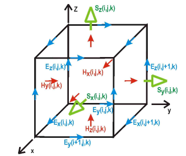
Figure 8: The placement and labeling of the EM fields and Poynting vector components in the Yee cell, adapted from Reference (Kunz and Luebbers 1993).

The numerical accuracy of Equation 11 was tested for the case of an EM pulse propagating through empty space where the deposited energy inside the Yee cell should be $0$. In the worst case, the accuracy of the method, measured as the deviation from $0$, was found to be less than 0.02 %, a negligible error compared, for example, to the accuracy of the dielectric properties of tissues.

Numerical computation of the absorbed energy was also validated by comparing the results obtained using Equation 11 with those obtained by analytical solution. For a normal incidence of an EM wave on a infinite conducting surface of a dielectric constant $\varepsilon=\varepsilon_{R}-i\varepsilon_{I}$, the transmitted energy flux or transmittance can be calculated as

$$T=1-{{(\sqrt{\varepsilon}_{R}-1)^{2}+\varepsilon_{I}}\over{(\sqrt{\varepsilon}_{R}+1)^{2}+\varepsilon_{I}}}$$ (13)

The dielectric constant for a muscle at a frequency of $\rm 7\;GHz$, the mid frequency of $\rm 3.1-10.6\;GHz$ range pulse, is $\varepsilon=46.9-i16.6$. For this dielectric constant, Equation 13 gives for the transmittance a value of $35\%$. Equation 11 gives for the transmittance of a $\rm 3.1-10.6\;GHz$ range UWB pulse $33\%$. This is as good as expected agreement taking into consideration that the absorbed energy is computed only to the depth of $\rm 20\;mm$ and that the transmittance of the UWB pulse was compared to transmittance of a plane wave having the pulse’s mid frequency.

7 Dissipation of Electromagnetic Pulse Energy Inside the Eye

The penetration of the EM pulses into a human eye is shown in Figures 9 and 10. As expected, the penetration depth decreases as the pulse’s frequency spectrum increases. In the case of the pulse in the lowest frequency range, as shown in Figure 9, significant energy penetrates about $\rm 10\;mm$ into the eye where it is, as a result of the complex eye structures, relatively nonhomogeneously absorbed. Surprisingly significant contribution to energy absorption modulation comes from, in computation, typically neglected structures as, for example, the iris. Also, unexpectedly, most of the energy in the cornea is absorbed next to the eye lids. The $\rm 22-29\;GHz$ range UWB pulse significantly penetrates into the eye only $\rm 2-3\;mm$ (Figure 10). Most of the energy is absorbed by the cornea with the energy absorption hot spots again immediately above or below the eye lids. The $\rm 57-64\;GHz$ range UWB pulse is almost entirely and uniformly absorbed by the cornea. While the energy absorption data exist for the entire eye volume, only selected data can be presented in this paper.

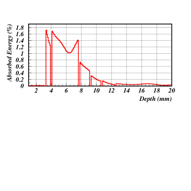
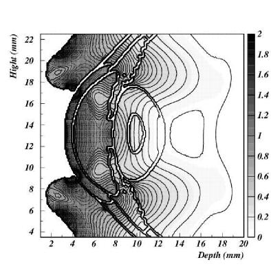
Figure 9: Contour plot of the density of the energy absorption across the vertical cross section of the eye in percentage of the total available energy for the $\rm 3.1-10.6\;GHz$ range UWB pulse. Distribution of the absorbed energy along the mid-line is shown in the top figure. From left to right separate regions corespond to cornea, anterior chamber, lens cortex, lens nucleus, lens cortex (again), and vitreous humor.

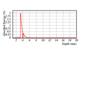
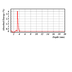
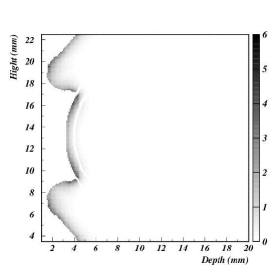
Figure 10: Contour plots of the density of the energy absorption across the vertical cross section of the eye in percentage of the total available energy for the $\rm 22-29\;GHz$ (left) and $\rm 57-64\;GHz$ (right) frequency range UWB pulses. Distributions of the absorbed energy along the mid-line are shown on the top. From left to right separate regions corespond to cornea and anterior chamber.

Most of the experimental work on the effects of eye exposure to electromagnetic radiation in the frequency range covered in this paper was performed using continuous waves. We will compare the results of the UWB pulse propagation with the results of the CW, restricting ourselves to the frequencies above $\rm 10\;GHz$. Above $\rm 10\;GHz$ experimental results exist for the exposure to $\rm 35\;GHz$ waves (Rosenthal et al 1977, Chalfin et al 2002) and $\rm 60\;GHz$ waves (Kues et al 1999, Kojima et al 2005). A short but detailed summary of the experiments, including the experimental apparatus, organic material, cellular environment, and possible electromagnetic interaction mechanisms can be found in Miller et al (2002).

Searching for any abnormal effects resulting from the eye exposure to UWB radiation, the computed distribution of the absorbed energy in the case of UWB exposure was compared to the energy distribution in the case of CW. As shown in Figure 11, no difference in the amount of absorbed energy was found when the $\rm 57-64\;GHz$ frequency range UWB pulse was compared to $\rm 60\;GHz$ CW, or when the $\rm 22-29\;GHz$ frequency range UWB pulse was compared to $\rm 22.5\;GHz$ CW, both corresponding to mid-frequency of the pulses spectra. When $3\rm 5\;GHz$ CW was compared to a $\rm 22-29\;GHz$ frequency range pulse (bottom of Figure 11), as expected, the pulse penetrated deeper into the eye due to its lower frequency spectrum. No extraordinary effects outside the consequences from the Fourier decomposition of the UWB pulse were observed. Two factors played a role in the energy dissipation of the UWB electromagnetic radiation: the frequency spectrum of the pulse and the dielectric properties of the exposed biological material at those frequencies.

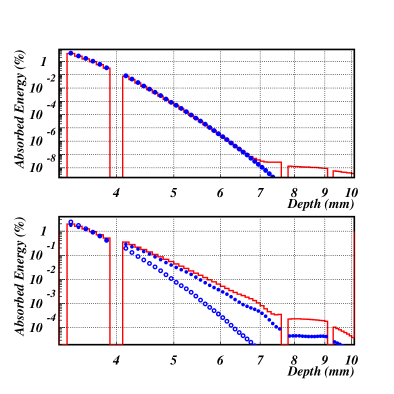
Figure 11: Top: comparison of the absorbed energy after exposure to $\rm 57-64\;GHz$ frequency range UWB pulse (red line) and after exposure to $\rm 60\;GHz$ CW (blue circles). Bottom: comparison of the absorbed energy after exposure to $\rm 22-29\;GHz$ frequency range UWB pulse (red line) and after exposure to $\rm 22.5\;GHz$ (filled blue circles) and $\rm 35\;GHz$ CW (hollow blue circles). From left to right separate regions corespond to cornea, anterior chamber, lens cortex, and lens nucleus.

The consequences of this study is summarized in the Table 2. As was shown, the energy in the material exposed to UWB electromagnetic radiation was absorbed in the same way as in the material exposed to a CW in the coresponding pulse frequency spectrum. The absorbed energy in the tissues was, in both cases, and in the same way, proportional to the total available EM energy.

The total available energy in the case of CW can be easily calculated from the Poynting vector

$$S={c\varepsilon_{0}\over 2}E_{0}^{2},$$ (14)

where $c$ is the speed of light, $\varepsilon_{0}$ the vacuum permittivity, and $E_{0}$ the CW electric field amplitude. The energy of the UWB pulse can be easily obtained by integration

$$S=c\varepsilon_{0}\int_{T}E(t)^{2}dt$$ (15)

over the pulse time duration $T$. $E(t)$ is the electric field at the time $t$. It is easy to see that, for the same field amplitude, the energy carried by the short EM pulses depends on the pulse repetition rate and it is always much smaller than the energy carried by the CW. The results are summarized in Table 2. Assuming the same exposure time, for the pulse repetition rate of 1MHz, the energy absorbed by the exposed material will be $\sim$ 0.01 % of the corresponding CW exposure, for the maximum repetition rate of  1 GHz, the energy absorbed will be $\sim$ 10 % of the coresponding CW energy. Any possible absorbed-dose-related health effects as a results of the exposure to UWB will be therefore reduced by one to many orders of magnitude compared to the health effects caused by the exposure to CW. To quote from Miller et al (2002): “ We want to close this section with a more general observation on the effects of UWB pulses. When we first started this work, there was speculation that even one UWB pulse might have serious effects on biological organisms. So far, we have exposed animals to over a quarter of a billion UWB pulses, and we have never seen any acute effects.”

Pulse Frequency Range (GHz)	RepRate: 1 MHz	RepRate: 1 GHz
$3.1-10.6$	0.011 %	11%
$22-29$	0.009 %	9 %
$57-64$	0.009 %	9 %

Table 2: Energy carried by the UWB pulse as a percentage of the energy carried by the CW of the same field amplitude, and in the same time interval. In one case $10^{6}$ and in the other $10^{9}$ pulses were generated in one second.

8 Conclusion

In this paper, we have performed full three dimensional FDTD calculations of the penetration of UWB electromagnetic pulses, authorized by the FCC for communications, radar imaging, and vehicle radars, into a human eye. Calculations included as detailed geometrical description of the eye as necessary and as accurate description of the physical properties of the eye tissue as allowed by existing data. The spatial resolution of $\rm 0.1\;mm$ side length of the Yee cell allowed reliable calculation of up to $\rm\sim 90\;GHz$ in frequency range in the dielectric.

To minimize the computation time, the electromagnetic interaction with dielectric material was modeled using the Piecewise-Linear Recursive Convolution method (PLRC) for Debye media. Dielectric properties of the eye tissues in the frequency range $\rm\leq 100\;GHz$ were formulated in terms of the Debye parametrization with the same accuracy as the accepted Cole-Cole parametrization.

The energy absorbed after the UWB exposure was evaluated over the entire eye volume and compared to the energy absorbed after the exposure to continuous electromagnetic waves. The energy in the material exposed to UWB electromagnetic radiation was absorbed in the same way as in the material exposed to a CW in the coresponding pulse frequency spectrum. We have found that, assuming the same field amplitude and the same exposure time, any possible dose dependent health effects as a results of the exposure to UWB radiation will be reduced by one to many orders of magnitude compared to the health effects caused by the exposure to CW. This finding is in agreement with the experiments carried out at the US Air Force Research Laboratory at Brooks (Miller et al 2002).

We can conclude that, based on the research described in this paper, any future applications of UWB pulses, for the purposes and in the frequency range approved by the FCC, pose less health risk compared to those applications being carried by the continuous electromagnetic radiation.

References

References

- [1]
- [2] [] Barnes F S and Greenebaum B eds. 2006 Handbook of Biological Effects of Electromagnetic Fields - third edition Boca Raton: CRC Press LLC.
- [3] [] Chalfin S, D’Andrea J A, Comeau P D, Belt M E and Hatcher D J 2002 Health Physics 83 83
- [4] [] Charles M W and Brown N 1975 Phys. Med. Biol. 20 202
- [5] [] de AlmeidaI M S and Carvalho L A 2007 Braz. J. Phys. 37 378
- [6] [] Federal Communications Commission 2002, News Release NRET0203, http://www.fcc.gov
- [7] [] Gabriel C 1996 Preprint AL/OE-TR-1996-0037, Armstrong Laboratory Brooks AFB
- [8] [] Gabriel C, Gabriel S, and Corthout E 1996 Phys. Med. Biol. 41 2231
- [9] [] Gabriel S, Lau R W and Gabriel C 1996 Phys. Med. Biol. 41 2251
- [10] [] Gustavsen B and Semlyen A 1999 IEEE Trans. Power Delivery 14 1052
- [11] [] Hu Q, Viswanadham S, Joshi R P, Schoenbach K H, Beebe S J and Blackmore P F 2005 Phys. Rev. E 71 031914
- [12] [] ICNIRP 1998 Health Physics 74 494
- [13] [] IEEE Standards Coordinating Committee 28 on Non-Ionizing Radiation Hazards: Standard for safety levels with respect to human exposure to radio frequency electromagnetic fields, 3 kHz to 300 GHz (ANSI/IEEE C95.1-1991), The Institute of Electrical and Electronics Engineers, New York; 1992.
- [14] [] Jackson J D 1999 Classical Electrodynamics New York:John Willey & Sons Inc.
- [15] [] Ji Z, Hagness S C, Booske J H, Mathur S, and Meltz M 2006 IEEE Transactions on Biomedical Engineering 53 780
- [16] [] Kojima M, Yamashiro Y, Hanazawa M, Sasaki H, Wake K, Watanabe S, Taki M, Kamimura Y and Sasaki K 2005 Proceedings of the XXVIIIth URSI General Assembly in New Delhi K02.9(470)
- [17] [] Kues H, D’Anna S A, Osiander R, Green W R and Monahan J C 1999 Bioelectromagnetics 20 463
- [18] [] Kunz K and Luebbers R 1993 The Finite Difference Time Domain Method for Electromagnetics Boca Raton: CRC Press LLC.
- [19] [] Landau L D and Lifshitz 1960 Electrodynamics of Continuous Media Reading: Addison-Wesley Inc.
- [20] [] Lotmar W 1971 J. Opt. Soc. Am. 61 1522
- [21] [] Luebbers R J, Hunsberger F, Kunz K S, Standler R B, and Schneider M 1990 IEEE Trans. Electromagn. Compat. 32 222
- [22] [] Luebbers R J, Hunsberger F, and Kunz K S 1991 IEEE Trans. Antennas Propagat. 39 29
- [23] [] Luebbers R J and Hunsberger F 1992 IEEE Trans. Antennas Propagat. 40 1297
- [24] [] Lugo G R N 2006 Modelos dispersivos para analisis de la propagacion de campos electromagneticos en tejidos biologicos Master thesis, Universidad Autonoma de Nuova Leon, Mexico
- [25] [] Miller R L, Murphy M R and Merritt J H 2002 Proceding of the 2nd International Workshop on Biological Effects of EMFs Rhodes, Greece; 2002:468-477.
- [26] [] Norrby S, Piers P, Campbell C and van der Mooren M 2007 Applied Optics accepted for publication
- [27] [] Polk C and Postow E eds. 1995 Handbook of Biological Effects of Electromagnetic Fields - second edition Boca Raton: CRC Press LLC.
- [28] [] Rosenthal S W, Birenbaum L, Kaplan I T, Metlay W, Snyder W Z and Zaret M M 1977 HEW Publication (FDA) 77-8010 110
- [29] [] Sadiku M N O 1992 Numerical Techniques in Electromagnetics Boca Raton: CRC Press LLC.
- [30] [] Schoenbach K H, Joshi R P, Kolb J F, Chen N, Stacey M, Blackmore P F, Buescher E S, and Beebe S J 2004 Proceedings of the IEEE 92 1122
- [31] [] Siedlecki D, Kasprzak H and Pierscionek B K 2004 Optics Letters 29 1197
- [32] [] Simicevic N and Haynie D T 2005 Phys. Med. Biol. 50 347
- [33] [] Simicevic N 2005 Phys. Med. Biol. 50 5041
- [34] [] Simicevic N 2007 Health Physics. The Radiation Safety Journal 92 574
- [35] [] Simicevic N 2007 http://caps.phys.latech.edu/neven/pmb/
- [36] [] Sullivan, D M 2000 Electromagnetic Simulation Using the FDTD Method New York: Institute of Electrical and Electronics Engineers.
- [37] [] Taylor J D ed. 1995 Introduction to Ultra-Wideband Radar Systems Boca Raton: CRC Press LLC.
- [38] [] Taflove A and Hagness S C 2000 Computational Electrodynamics: The Finite-Difference Time-Domain Method, 2nd ed. Norwood: Artech House.
- [39] [] Yee K S 1966 IEEE Trans. Antennas Propagat. AP-14 302
- [40] [] Zastrow E, Davis S K and Hagness S C 2007 Microwave and Optical Technology Letters 49 221
- [41]