Photometric redshift error estimators

Abstract

Photometric redshift (photo-z) estimates are playing an increasingly important role in extragalactic astronomy and cosmology. Crucial to many photo-z applications is the accurate quantification of photometric redshift errors and their distributions, including identification of likely catastrophic failures in photo-z estimates. We consider several methods of estimating photo-z errors and propose new training-set based error estimators based on spectroscopic training set data. Using data from the Sloan Digital Sky Survey and simulations of the Dark Energy Survey as examples, we show that this method provides a robust, relatively unbiased estimate of photo-z errors. We show that culling objects with large, accurately estimated photo-z errors from a sample can reduce the incidence of catastrophic photo-z failures.

1. Introduction

While spectroscopic redshifts have now been measured for over one million galaxies, in recent years digital sky surveys have obtained multi-band imaging for over a hundred million galaxies. Deep, wide-area surveys planned for the next decade will increase the number of galaxies with multi-band photometry to a few billion. Over the last decade, substantial effort has gone into developing photometric redshift (photo-z) techniques, which use multi-band photometry to estimate approximate galaxy redshifts (Connolly et al. 1995; Bolzonella et al. 2000; Benitez 2000; Collister & Lahav 2004; Wadadekar 2005). For many applications in extragalactic astronomy and cosmology, the precision achieved by photometric redshifts is sufficient, provided one can accurately characterize the uncertainties in the photo-z estimates, i.e., the photo-z errors. A number of recent papers have considered the effects of photo-z errors on cosmological probes including baryon acoustic oscillation (Zhan & Knox 2006), weak lensing tomography (Huterer et al. 2006; Ma et al. 2006), supernovae (Huterer et al. 2004) and galaxy clusters (Huterer et al. 2004; Lima & Hu 2007).

A number of methods have been proposed to characterize photometric redshift errors to date. They can be roughly divided into two categories: methods based on estimating statistical errors in template fitting, e.g., the $\chi^{2}$ method and its Bayesian counterparts (Bolzonella et al. 2000; Benitez 2000); and methods that explicitly propagate errors in the input parameters, typically magnitudes or colors, through the photo-z estimator (e.g., Brunner et al. 1999; Hsieh et al. 2005; Collister & Lahav 2004).

The error in a photometric redshift estimate $z_{\rm phot}$  is simply the difference between the photo-z estimate and the true (hereafter, spectroscopic) redshift, $\Delta z=$$z_{\rm phot}$$-$$z_{\rm spec}$. In practice, the errors for the vast majority of objects in a deep photometric sample are unknown, since the spectroscopic redshifts are not measured. Our goal is to devise an estimator of $\Delta z$ that has desirable statistical properties, e.g., minimum bias and variance, based on whatever information is at hand. Given a photo-z estimate, an error estimator should give the range of redshifts over which the true redshift will be found at some confidence level.

In most cases, spectroscopic redshifts are available for a small subset of the photometric sample. Such spectroscopic samples are often used as training sets for empirical or machine-based learning photo-z estimators. In this paper, we develop methods of photo-z error estimation that are based on the use of spectroscopic training sets to accurately characterize the error distribution. We show that training-set based error estimators outperform other commonly used methods when a representative training set is available and that they are competitive even when the training set is not fully representative of the photometric sample. In cases where the magnitude errors are not well determined, we show that the relative advantages of the new training-set based methods are further increased.

This paper is organized as follows. In §2, we describe the data sets that we use in this work. In §3, we introduce the training-set based error estimators and their implementations, as well as their advantages and disadvantages. For comparison, we review the traditional error estimators in §4 and highlight the key differences between them and the training-set based error estimators. We show in §5 that the over-all photo-z scatter and outlier fraction can be significantly improved by culling objects with high estimated photo-z errors, possibly leading to improved results in analyses that rely on photo-z’s. Finally, we offer concluding remarks in §6.

2. Test Methods and Data

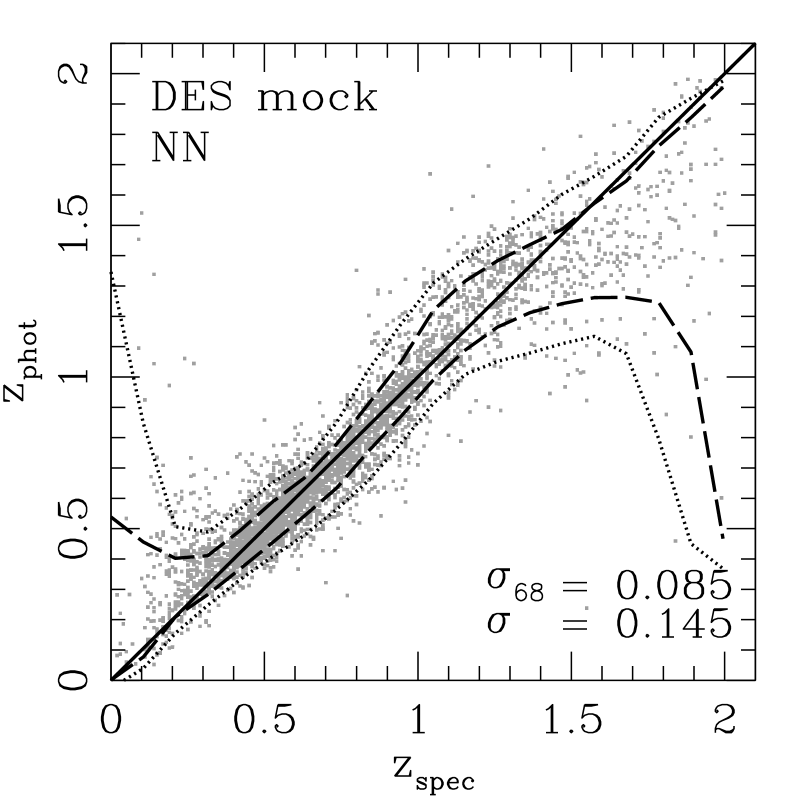
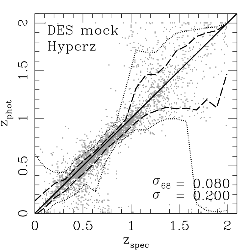
Figure 1.— Photometric versus spectroscopic redshift for the DES mock catalog photometric set, calculated using the Neural Network (top panel) and Hyperz (bottom panel) methods. The dashed and dotted curves enclose 68% and 95% of the points in each $z_{\rm spec}$  bin. In the lower right of each panel, $\sigma$ is the rms photo-z scatter averaged over all $N$ objects in the photometric set , $\sigma^{2}=(1/N)\Sigma_{i=1}^{N}(\Delta z^{i})^{2}$, and $\sigma_{68}$ is the range containing 68% of the validation set objects in the distribution of $\Delta z$. The Hyperz photo-z’s for the DES mock catalog are calculated with $z_{\rm max}$ set to 2.

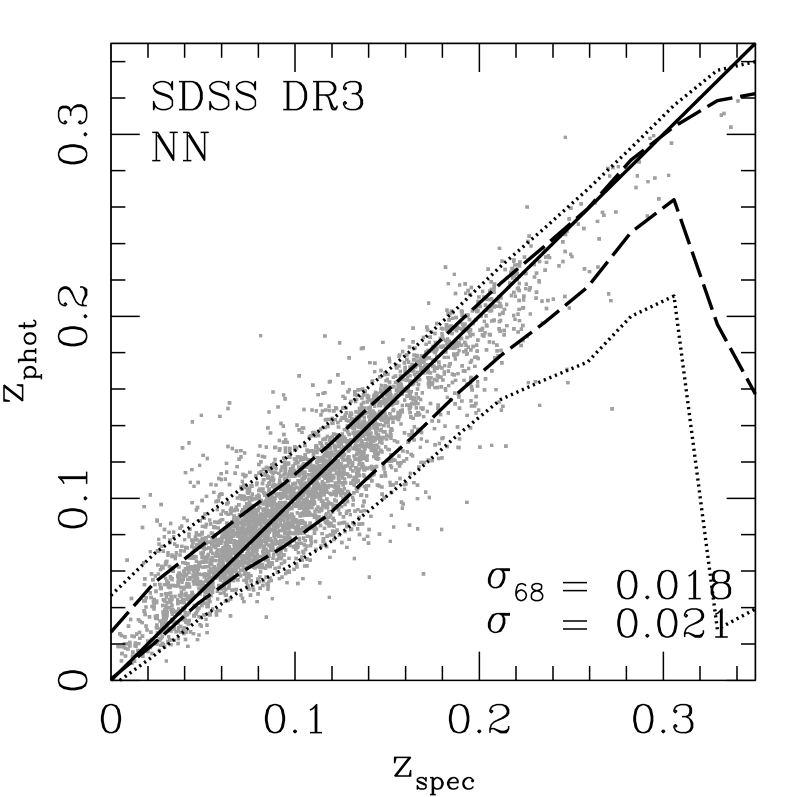
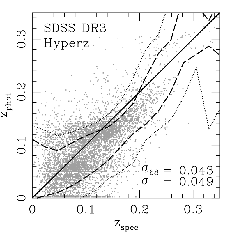
Figure 2.— Photo-z versus spectroscopic redshift for the SDSS DR3 photometric set calculated using the Neural Network (top panel) and Hyperz (bottom panel). The Hyperz photo-z’s for the SDSS catalog are calculated with $z_{\rm max}$ set to 0.4.

In order to fairly compare the qualities of various photometric redshift error estimators, we have compiled two galaxy photometric catalogs. Each catalog consists of spectroscopic redshifts, magnitudes in several chosen filter passbands, and magnitude errors.

The first catalog is a simulated data set created to resemble observations of the proposed Dark Energy Survey (DES) (The Dark Energy Survey Collaboration 2005). The DES is a 5000 square degree survey in 5 optical passbands ($grizY$) with a magnitude limit of $i\approx 24$, to be carried out using a new camera on the CTIO 4-meter telescope. The goal of the survey is to measure the equation of state of dark energy using several techniques: clusters, weak lensing, angular galaxy clustering (baryon acoustic oscillations), and supernovae. Since DES will observe $\sim 300$ million galaxies, the redshifts must be obtained using photometric methods. The DES optical survey will be complemented in the near-infrared by the VISTA Hemisphere Survey, an ESO Public Survey on the VISTA 4-meter telescope that will cover the survey area in $J,H$, and $Ks$. While the color information provided by $grizYJHKs$ photometry leads to improved photo-z estimates compared to optical-only imaging, for simplicity and purposes of illustration the mock catalog we use here contains only $griz$ magnitudes.

The simulated DES catalog contains 200,000 galaxies with $z<2$ and with $20<i<24$. The magnitude and redshift distributions are derived from the galaxy luminosity function measurements of Lin et al. (1999) and Poli et al. (2003), while the galaxy SED type distribution is obtained from measurements of the HDF-N/GOODS field (Capak et al. 2004; Wirth et al. 2004; Cowie et al. 2004). The galaxy colors are generated using the four Coleman et al. (1980) templates–E, Sbc, Scd, Im–extended to the UV and NIR using synthetic templates from Bruzual & Charlot (1993). To improve the sampling and coverage of color space, we create additional templates by interpolating between adjacent templates or by extrapolating from the E and Im templates.

The second test catalog we use is based on the Sloan Digital Sky Survey (SDSS) Data Release 3 (Abazajian et al. 2003). Although this catalog has been superceded by later data releases (Adelman-McCarthy et al. 2007), for which we have published a photo-z catalog (Oyaizu et al. 2007), it nevertheless provides a useful testbed for studies of photo-z errors. This SDSS catalog contains spectroscopic redshifts and magnitudes in $ugriz$ passbands for $292,964$ galaxies from the main spectroscopic sample, which is flux-limited to $r<17.77$. Because this sample is confined to low redshift, $z\lesssim 0.3$, most of the strong features of galaxy spectra targeted by photometric redshift estimators fall within the wavelength range covered by the filters. A notable exception is the Lyman alpha emitters at $z>2.5$. However, the fraction of these high redshift objects in our sample is too small to have measurable effects on our results.

We calculate photometric redshifts for these catalogs using two methods, a Neural Network (NN) method and the $\chi^{2}$ based spectral template fitting package Hyperz (Bolzonella et al. 2000). The NN technique is a training-set method based on fitting a parametrized function, represented by a feed-forward multilayer perceptron (FFMP) neural network, to the redshift-magnitude relation embodied in a spectroscopic training set. The implementation is the same as the one described in Oyaizu et al. (2007) for the SDSS DR6 photo-z catalog, except that the network configurations are different: here we use a 4:15:15:15:1 network for the DES catalog and a 5:15:15:15:1 network for the SDSS catalog. Figures 1 and 2 show the resulting photometric redshifts plotted against spectroscopic redshifts for all catalogs used in this study.

We split the DES and SDSS catalogs into three independent catalogs each, labeled training, validation, and photometric sets. The sizes of these sets are 50,000, 50,000, and 100,000 for the DES and 100,000, 92,964, and 100,000 for the SDSS. Except where noted below (§3.3), these subsets are drawn at random from the photometric samples, i.e., they are each statistically representative of the full samples. When the photo-z’s are determined using the NN training-set method, we use the training and validation sets to determine the mapping from magnitudes to redshifts and magnitudes to redshift errors. The resulting mapping is then applied to the photometric set for comparison of the training-set error estimator against other error estimation methods. Splitting the catalogs ensures that the training-set error methods are not given unfair advantage with respect to the other error estimators. When we estimate photo-z’s and photo-z errors using template methods, we apply the methods directly to the photometric set.

3. Error estimates using training sets

Training set based photo-z estimators (e.g., Connolly et al. 1995; Csabai et al. 2003; Collister & Lahav 2004) use a spectroscopic training set, typically a subset of the photometric sample, to derive a functional relation between redshift and photometric observables (e.g., magnitudes) which is then applied to the photometric sample of interest. In the same spirit, we can also use a training set to derive an estimate of the photo-z error, that is, a relation between photo-z error and some photometric observables. Note that the error estimator does not need to make use of the same observables as the photo-z estimator. In fact, we stress that the empirical photo-z error estimators are independent of the method used to estimate photometric redshifts themselves: training-set based error estimators can be applied to either empirical (training set) or template-based photo-z estimates. The assumption underlying the training-set based error estimator is that there is a functional relationship between some set of photometric observables and photo-z error and that this relationship for the training set data is reasonably representative of the relationship for the photometric sample as a whole.

In the following subsections, we describe and test two basic techniques that use a spectroscopic training set to estimate photo-z errors. Both techniques are based on the simple observation that objects with similar magnitudes in a photometric survey tend to have similar photometric errors, and such magnitude errors are typically the largest contributors to photometric redshift error. Therefore, objects with similar multi-band magnitudes will tend to have similar photo-z errors. Moreover, such neighbors in magnitude space, having similar colors, usually (but not always) correspond to galaxies with similar SEDs. Photo-z errors depend strongly on SED type, since the quality of photo-z estimates is related to the presence of strong and broad spectral features. We can therefore group objects in a spectroscopic training set according to their magnitudes and determine the photo-z error as a function of the magnitudes using the training set. For each object in the photometric set, we then find the objects in the training set that are near it in magnitude-space and associate some weighted mean of the measured errors for these training-set neighbors to it. The two methods introduced below differ in the method of grouping the galaxies.

Figure 3.— Upper panels: Estimated error vs empirical error for a) DES photometric set using Kd-tree error estimate, b) SDSS using Kd-tree, c) DES using Nearest Neighbor error (NNE) estimate, and d) SDSS using NNE. In all four cases, the neural network method was used to estimate the photo-z’s. Lower panels: Corresponding distributions of $(z_{\rm phot}-z_{\rm spec})/\sigma_{\rm est}$, where $\sigma_{\rm est}$ is the photo-z error estimate for each galaxy. Solid histograms show the distributions, dashed curves are Gaussian fits to the distributions.

3.1. Kd-tree Error Estimator

The first photo-z error method we consider uses a Kd-tree algorithm to bin training-set objects in magnitude space. A Kd-tree (short for K-dimensional tree) is a general data organization and classification algorithm that is suited for efficiently partitioning data points in multi-dimensional parameter spaces. In our implementation, the training set is partitioned into two bins at the median value of the first photometric parameter (which we choose to be $u$ mag for SDSS, $g$ for DES). For each bin, the objects within the bin are further partitioned at the median of the second parameter (here $g$ for SDSS, $r$ for DES), resulting in $2^{2}=4$ bins. This process is continued for the photometric parameters of interest (here the 5 magnitudes for SDSS and 4 for DES). We then return to the first parameter, partition each bin at the median of the first parameter for that bin, cycle again through the parameters, and continue subdividing until the number of objects in a bin becomes sufficiently small. Once the partitioning is completed, we calculate the 68% width of the error distribution centered about $z_{\rm phot}-z_{\rm spec}=0$ for each bin and declare that to be the photo-z error estimate for objects in the photometric sample that fall within that bin.

Because the Kd-tree bins are always partitioned at the median value of the object distribution in some parameter, the number of training-set objects per bin, $N_{b}$, is nearly constant from bin to bin. This constancy ensures a nearly uniform shot-noise uncertainty ($\propto 1/\sqrt{N_{b}}$) on the estimates of the photo-z errors. While this statistical uncertainty is minimized by having many objects per bin, large bins are “non-local” in multi-magnitude space, and the training-set based error estimator is predicated on the locality assumption that similar magnitudes imply similar errors. Therefore, the optimal bin size should be as small as possible (or smaller than the scale over which the error distribution changes appreciably) but large enough that the shot-noise error is not large compared to the error induced by non-locality of the bin. For the training set samples we consider here, we find that $N_{b}\simeq 100$ objects per bin is nearly optimal. The size of the training set can also change the locality of the nearest $N_{b}$ neighbors, and in general, the required locality depends on the first derivative of the redshift-magnitude relationship. Because such relationships are dependent on numerous factors, such as filter choice, selection function, and magnitude errors, we cannot provide a general requirement for the training set size. We note, however, that in both DES mock and SDSS catalogs, we find virtually no improvement in error estimator quality when the training set size is larger than 20,000 galaxies.

Figures 3a and 3b show the results of applying the Kd-tree error estimator to the DES and SDSS photometric sets. In these cases, the neural network (NN) method was used for the photo-z estimates. The photo-z errors are estimated using a Kd-tree with 512 bins for the DES catalog and 1024 bins for the SDSS catalog, corresponding to $N_{b}\simeq 97$ training-set objects per bin in each case. The top panels of Figure 3 show the photo-z error estimates vs. the measured or “empirical” errors. In order to compute the empirical error, we first sort the galaxies according to their estimated error. Next, we bin the galaxies into bins of 100 objects starting from the galaxy with the smallest estimated error, and call the average estimated error of the galaxies within a bin the “estimated error” of the bin, which is plotted on the vertical axis of Figure 3. Finally, we compute the 68% width of the $|z_{\rm phot}-z_{\rm spec}|/\sigma_{\rm est}$ distrubtion of each bin, and call it the “empirical error” of the bin. The assumption here is that if the error estimator is working properly, those objects with similar estimated error should follow similar underlying error distributions, and the underlying distribution should have a width that is well-approximated by the estimated error. As the figure shows, the estimated Kd-tree error correlates well with the true error, with almost no apparent bias and relatively small scatter.

The solid histograms in the lower panels of Figure 3 show the corresponding distributions of $(z_{\rm phot}-z_{\rm spec})/\sigma_{\rm est}$, where $\sigma_{\rm est}$ is the Kd-tree error estimate. The dashed curves in these panels show Gaussian fits to the error distributions; we also indicate the best-fit Gaussian means ($\mu_{\rm Gauss}$) and standard deviations ($\sigma_{\rm Gauss}$) as well as the $\sigma_{68}$ widths (about zero) of the distributions (not the fits). The fits give equal weight to each bin of the distributions and ignore objects for which $\sigma_{\rm est}=0$. There is no a priori reason for these error distributions to be Gaussian. Nevertheless, for the Kd-tree error estimator, the error distributions are very close to Gaussians, except for small tails seen for both the DES and SDSS catalogs. The tails are signatures of catastrophic photo-z failures: due to photometric errors, an intrinsically underluminous, red galaxy at low redshift, for example, may “scatter into” a bin mostly populated (in the training set) by intrinsically luminous, blue galaxies at much higher redshift. In such degenerate cases, the photo-z error is large, and the Kd-tree error underestimates the true error: in this example, the Kd-tree error assigned to the red galaxy interloper would be dominated by the small errors of the blue galaxies in that bin. With a sufficiently large training set, one could hope to identify such problematic bins in magnitude space, since the photo-z error distributions in the training set for those bins would show anomalous tails.

A disadvantage of the Kd-tree method is the fact that the estimated error is discrete. There can only be as many different error estimates as there are Kd-tree bins, and this limits the resolution of the estimated photo-z errors, especially for objects with large photo-z errors as seen by the lack of high Kd-tree estimated errors in Figure 3. This problem can in principle be alleviated by using more Kd-tree bins. However, as noted above, for fixed training set size, the number of bins is limited by the requirement that each bin should contain enough training-set objects to determine the error with small shot-noise uncertainty.

3.2. Nearest Neighbor Error estimator

While the Kd-tree error estimator was seen to have good statistical properties, we have found that a Nearest Neighbor Error (NNE) estimator performs even better. Note that the NNE has in principle nothing to do with Neural Networks (NN), and the readers should be careful not to confuse the similar acronyms. In this method, for each object in the photometric set, we estimate the photo-z error by using the 68% spread of the error distribution of its $N_{\rm nei}$ nearest neighbors in the training set. Here, nearness in magnitude space is defined using the Euclidean metric: given two objects with two sets of measured magnitudes ${\textbf{m}_{1}}$ and ${\textbf{m}_{2}}$, we define the distance between them by

$$D^{2}=|{\bf m_{1}}-{\bf m_{2}}|^{2}=\sum_{\mu=1}^{N_{m}}(m_{1}^{\mu}-m_{2}^{\mu})^{2}~{},$$ (1)

where $N_{m}$ denotes the number of magnitudes (different passbands) measured for each object. In contrast to the Kd-tree method, in NNE each object in the photometric set defines its own “bin.”

The choice of the number of nearest neighbors ($N_{\rm nei}$) to use is analogous to the choice of the number of bins in the Kd-tree error estimate. We prefer to keep the number of neighbors constant for all objects in the photometric set, since the shot noise of the resulting error estimate is then fixed. As with the Kd-tree method, one should choose $N_{\rm nei}$ large enough to keep the shot noise of the estimate under control but small enough so that the error estimate remains relatively local in magnitude space. For the samples we have tested in this analysis, we again find that $N_{nei}\simeq 100$ training-set neighbors is nearly optimal.

The upper panels of Figures 3c and 3d show the results of applying the NNE estimation method to the DES and SDSS catalogs. The discreteness that was a concern for the Kd-tree error estimate is not present in the NNE method. Moreover, the NNE error displays tighter correlation with the empirical error, because a nearest-neighbor bin for a photometric object is almost always more local in magnitude space than a Kd-tree bin for the same object. The lower panels of the same Figures show that the error distributions are reasonably well fit by Gaussians, with widths that are within 5% of the expected width $\sigma_{\rm Gauss}=1$. Non-Gaussian tails similar to those seen in the Kd-tree error distributions are also present in the NNE error distributions, for the same reasons.

Figure 4.— Left: Estimated Error vs. empirical error for NNE applied to the DES catalog with Hyperz photo-z’s. Right: Error distribution for the same data.

As noted above, the NNE and the Kd-tree error methods can be used in conjunction with any photo-z estimator, either training-set or template-based, provided there exists a subset of the photometric sample with spectroscopic redshifts. As an illustration, we use the Hyperz template fitting method to calculate photometric redshifts for the full DES mock catalog (shown in the lower panel of Fig. 1). We then use 50,000 objects from the DES catalog as a training set for NNE and calculate photo-z errors for the remaining photometric objects. Figure 4 shows the estimated vs. empirical error (left panel) and the error distribution (right panel) for this example. The NNE error estimate works well, though as before it results in an underestimate when the errors are very large ($\Delta z>0.25$). The error distribution is not as well fit by a Gaussian in this case; this is not surprising, since the photo-z estimate in this case has a net bias of $\sim 23\%$. However, the error estimator is able to account for the bias and is still able to predict the error to within 12% in $\sigma_{\rm Gauss}$. This ability to include the bias in the error estimates makes the training set error estimate approach particularly powerful compared to methods based on magnitude error propagation (see §4.2).

In our implementation of the NNE, computation of the NNE is expensive compared to the Kd-tree method. In the naive implementation, computation time to find the nearest objects scales as $N_{\rm T}N_{\rm P}$, where $N_{\rm T}$ and $N_{\rm P}$ are the number of objects in the training set and the photometric set, respectively (see, e.g., Press et al. 1992). In contrast, the Kd-tree method scales as $N_{\rm P}\log N_{\rm T}$. For most training-set photo-z methods, including the Neural Network, the computation time scales as $N_{\rm P}$. Therefore, for a sizeable training set ($N_{\rm T}\sim 10,000$ objects), the NNE computation dominates the time involved in estimating the photo-z’s and their errors. Fortunately, the method is trivially parallelizable, because the NNE calculation of one object in the photometric set is independent of all the other objects in the same set. Taking advantage of this parallelization, the NNE estimator has been successfully applied to a data set as large as the SDSS DR6 (Adelman-McCarthy et al. 2007) containing more than 78 million galaxies with Neural Net photo-z’s.(Oyaizu et al. 2007). In addition, tree-structured nearest neighbor search methods, such as the Cover-Tree (Baygelzimer et al. 2006), can be used to improve the computation time to $O(N_{\rm P}\log N_{\rm T})$, essentially eliminating the difference between the Kd-tree and NNE methods.

3.3. Non-representative training set

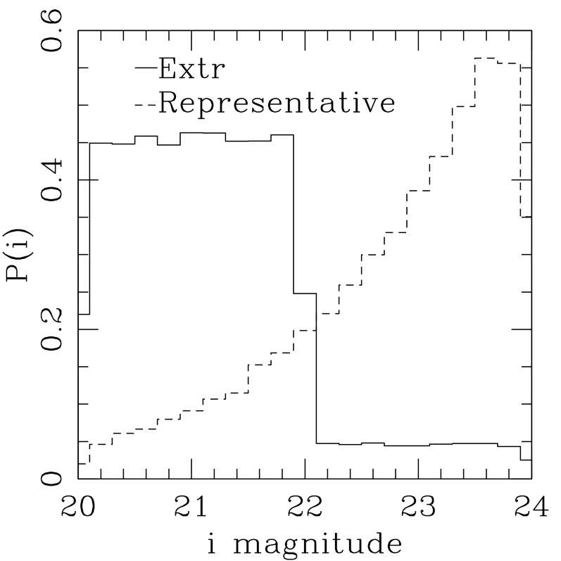
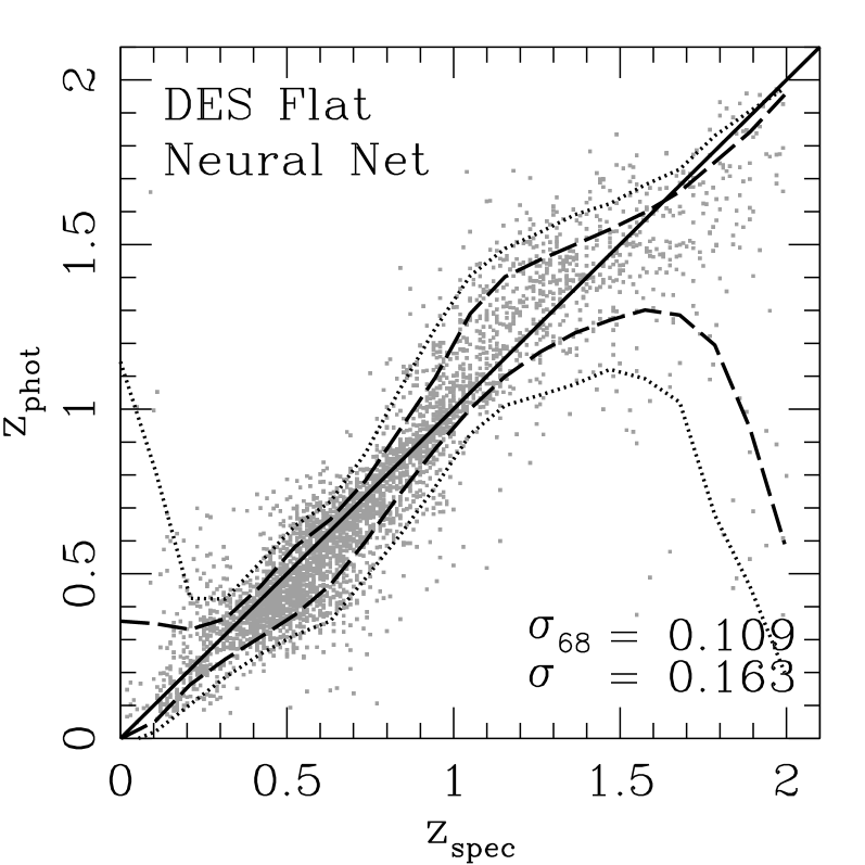
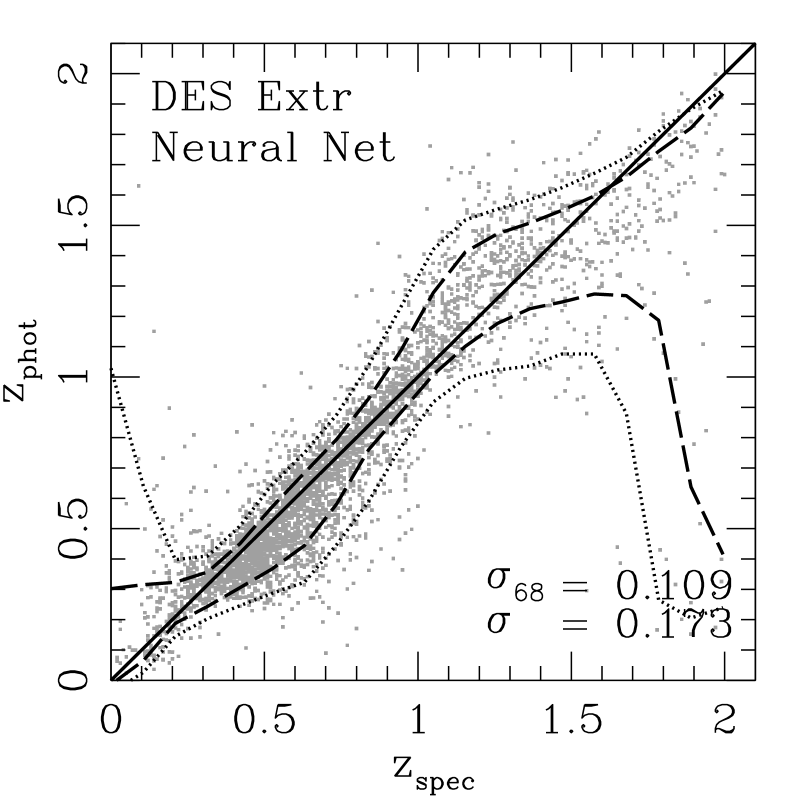
Figure 5.— Top row: $i$-magnitude distribution for the Flat and Extr non-representative training sets. The representative $i$-magnitude distribution is plotted in dashed lines for comparison. Bottom row: The Neural Network $z_{\rm phot}$ vs $z_{\rm spec}$ of the DES mock photometric set calculated using DES Flat training set (left panel) and DES Extr training set (right panel).

Figure 6.— Top row: NNE error vs empirical error calculated using two non-representative training sets. Bottom row: Error residual distributions.

The training-set based error estimators we have introduced rely on the spectroscopic training set to characterize the errors of the photometric set. Hence, the quality of the error estimate depends in principle on the degree to which the training set is a representative subsample of the photometric set. Since spectroscopic samples often are not simply random subsets of the parent photometric samples from which they are drawn, one might have concerns about the robustness of these error estimates. Here, we consider cases of non-representative training sets and show that the training-set error estimators perform satisfactorily provided the training set covers the full magnitude range of the photometric sample.

In order to illustrate the issue, we have constructed two non-representative training sets using the DES catalog generator. One training set (labelled Flat) has a flat $i$-magnitude distribution at $i<24$ instead of the increasing distribution characteristic of a flux-limited sample; bright (faint) objects are over- (under-)represented compared to the photometric sample. The second training set (labelled Extr) has an $i$-magnitude distribution highly skewed to bright magnitudes, $i<22$, since a spectroscopic set typically does not go as faint as the corresponding photometric sample. Both training sets have flat redshift and SED type distributions, differing from those of the fiducial DES mock catalog. The $i$-magnitude distributions, as well as the $z_{\rm phot}$ vs $z_{\rm spec}$ plots, are shown in Figure 5. Each training set contains 50,000 galaxies. We used the training sets to derive Neural Network photo-z solutions, which were then used to estimate photo-z’s for the DES mock photometric catalog. Photo-z errors were estimated using the NNE method, again using the same non-representative training sets in each case. In Fig. 6, we show the estimated vs. empirical error (top panels) and the error distributions (bottom panels) for the two cases. We see that the NNE error method estimates the errors correctly at the $\sim 10\%$ level while maintaining Gaussianity in both cases. In the case of the Flat training set, the error accuracy degradation is less than 1% compared to the representative training case. Given the fact that the Neural Network photo-z quality is itself degraded by $\sim 10\%$ compared to the representative case in scatter, these results show that the NNE error estimator is robust against differing distributions of the training and photometric sets.

A possible approach to the issue of non-representative training sets would be to resample or weight the training-set objects to obtain a distribution that matches the distribution of photometric observables (magnitudes, colors, etc.) of the photometric sample. In the case of the DES catalog and the two non-representative training sets used above, this resampling results in a marginal improvement in the error estimate at the $\sim 2\%$ level in both $\sigma_{68}$ and $\sigma_{\rm Gauss}$. We plan to offer further discussions and test results in subsequent articles, currently in preparation (Lima et al. 2008; Cunha et al. 2008).

4. Comparison with other error estimators

Other photo-z error estimators have been proposed in the literature. Two commonly used estimators are the $\chi^{2}$ error in template fitting methods, such as Hyperz (Bolzonella et al. 2000), and the propagation of magnitude errors that is found in, for example, ANNz (Collister & Lahav 2004). In this section, we discuss the performance of these error estimators and consider the advantages and disadvantages of our training-set based error estimators compared to these methods.

4.1. $\chi^{2}$ error estimate

Figure 7.— Left: $\chi^{2}$ estimated error vs empirical error for the DES mock catalog, using the Hyperz photo-z estimator. Right: $\chi^{2}$ error residual distribution, along with Gaussian fit. For the comparable training-set error, see Fig. 4.

Template-fitting photo-z methods often use $\chi^{2}$ minimization to determine the best-fit $z_{\rm phot}$ and spectral type. The quantity to be minimized is

$$\chi^{2}=\sum_{k=1}^{N_{\rm m}}\left[\frac{F_{\rm obs}^{k}-a\cdot F_{\rm temp}^{k}(z)}{\sigma_{F}^{k}}\right]^{2},$$ (2)

where $F_{\rm obs}^{k}$ is the observed flux in passband $k$, $\sigma_{\rm F}^{k}$ is the corresponding uncertainty in the flux, $F_{\rm temp}^{k}(z)$ is the flux of a template SED redshifted to a given $z$, $a$ is a normalization factor, and $N_{\rm m}$ is the number of passbands in which measurements are available. This statistic is minimized over redshift and over the set of template SEDs.

When a model being fit to data is linear in the fit parameters, the probability distribution for the $\chi^{2}$ statistic is the chi-square probability distribution for $\nu$ degrees of freedom, $P(\chi^{2}|\nu)$ (Press et al. 1992). Given the value of $\chi^{2}=\chi^{2}_{\rm min}$ that minimizes Eq. 2, the corresponding $P(\chi_{\rm min}^{2}|\nu)$ gives the probability that the observed $\chi^{2}$ for a correct model should be less than $\chi^{2}_{\rm min}$. This probability can be used to calculate redshift confidence intervals. Given a confidence level $\alpha$ ($0<\alpha<1$), define the quantity $\Delta_{\chi^{2}}$ such that (Avni 1976)

$$P(\chi^{2}\leq\Delta_{\chi^{2}}|\nu)=\alpha.$$ (3)

The level-$\alpha$ $z_{\rm phot}$ confidence interval is given by the set of all redshifts for which

$$\chi^{2}(z)-\chi^{2}_{\rm min}\leq\Delta_{\chi^{2}}~{},$$ (4)

where $\chi^{2}(z)$ is minimized over spectral type and the coefficient $a$. That is, $\Delta_{\chi^{2}}$ is simply the increment in $\chi^{2}$ required to cover the region of parameter space with redshift confidence $\alpha$. Here, we are interested in comparing the 68% confidence interval of the photometric redshift, so we set the parameter $\alpha=0.68$.

In Figure 7, we show the $\chi^{2}$-estimated error vs. empirical error and the residual error distribution for the Hyperz photo-z estimator applied to the DES mock catalog. The $\chi^{2}$ error underestimates the true error by about a factor of two. Furthermore, the distribution of the error residual divided by the estimated error is decidedly non-Gaussian, exhibiting strong tails. We attribute the underestimate to the fact that the chi-square distribution is not a realistic description of the true photo-z error distribution, given the relatively strong degeneracies present in the catalog. In a test using an artificial mock catalog containing only early-type galaxies, in which the degeneracy between redshift and galaxy SED type is removed, we found that the $\chi^{2}$ estimator was accurate at the $\sim 30$% level. In addition, the model used in the $\chi^{2}$ error estimator assumes that the fitting function, $F_{\rm temp}^{k}(z)$, is linear in the fitting parameters, namely the redshift. In reality, the template fitting functions are highly non-linear, and therefore it is not surprising that the $\chi^{2}$ error estimator does not robustly predict the correct errors.

We also tried to compute $\chi^{2}$ errors for Hyperz applied to the SDSS catalog, but we were not able to obtain sensible estimates. We found no discernible correlation between the $\chi^{2}$ errors and the true errors of the photo-z estimate. We discuss this issue further at the end of section 4.2.

4.2. Error estimate from Magnitude Derivative (MDE)

Figure 8.— Left: MDE error vs empirical error for the DES mock catalog, using the NN photo-z estimate. Right: Error residual distribution for MDE error for the DES mock catalog. For comparison with the training-set error estimators, see Figs. 3a,c.

The basic assumption underlying photo-z estimates is that there is a one-to-one mapping from photometric observables, e.g., magnitudes, to redshift. In training-set photo-z methods, this mapping is given by an explicit, usually analytic, function of magnitudes $m^{\mu}$ and fit coefficients $c_{\rm k}$,

$$z_{\rm phot}=z_{\rm phot}(c_{\rm k},m^{\mu})~{},$$ (5)

where the $c_{\rm k}$ are determined from the spectroscopic training set by minimizing a score function, a measure of the error residuals of the photo-z estimates. To first order, we can propagate the coefficient errors $\sigma_{c_{k}}$ and the magnitude errors $\sigma_{m}$ to the photo-z errors $\sigma_{z}$ as

$$\sigma_{z}^{2}=\sum_{k=1}^{N_{c}}\left(\frac{\partial z_{\rm phot}}{\partial c_{k}}\right)^{2}\sigma_{c_{k}}^{2}+\sum_{\mu=1}^{N_{m}}\left(\frac{\partial z_{\rm phot}}{\partial m^{\mu}}\right)^{2}\sigma_{m^{\mu}}^{2}~{}.$$ (6)

If the training set is sufficiently large (say, $\sim 10,000$ objects), the photo-z errors due to errors in the model fit coefficients are typically negligible compared to those arising from magnitude error propagation. Therefore we will concentrate on the latter and define the Magnitude Derivative error (MDE) as the second term in Eqn. 6 (Collister & Lahav 2004). For polynomial fitting and NN photo-z methods, analytic expressions for the derivatives (see, e.g., Bishop (1995) for the case of NN) can be used. However, we may also calculate these derivatives by finite difference, in which case MDE can be applied to any photo-z estimation method, including template fits.

Figure 8 shows the performance of the MDE error calculation for the DES mock catalog using neural network photo-z’s. MDE errors underestimate the true error by approximately 40% for this case. Although the error residuals are nearly Gaussian, the tails of the error distribution are more pronounced than the tails for the NNE error, signaling the failure of MDE to correctly identify catastrophic photo-z errors.

Collister & Lahav (2004) identify a second source of error in neural network photo-z’s: in the training process, the score function typically has many local minima with similar values. As a result, networks that start the minimization process at different initial values for the fit coefficients can end up in different local minima, resulting in slightly different photo-z estimates for the same input magnitudes. The variance in photo-z estimates due to this effect is an additional contribution to the photo-z error. By retraining our networks with different initial conditions, we find that the contribution of such an effect to the photo-z error is small ($<1\%$ of MDE) for our two catalogs, not enough to account for the underestimate of the MDE errors when applied to neural network photo-z estimates.

The $\chi^{2}$ and MDE error estimators are both predicated on the accuracy of the quoted magnitude errors. However, photometric errors are often difficult to estimate accurately (e.g., Scranton et al. 2005). The problem is further exacerbated if the magnitude errors in different passbands are correlated with each other, thereby violating the assumptions made in the $\chi^{2}$ fit and in magnitude error propagation. Because of these difficulties, the MDE errors applied to the NN photo-z estimates for the SDSS catalog are only weakly correlated with the true errors, similar to the case of $\chi^{2}$ error applied to the SDSS. A key advantage of the training-set based error estimators is that they do not depend on the measured magnitude errors.

5. Reducing Catastrophic Outliers: Culling objects by estimated error

Figure 9.— Top: Reduction in photo-z scatter $\sigma$ when objects with large estimated photo-z errors are culled from the sample, using two photo-z estimators, NN and Hyperz, and four error estimators, NNE, Kd-tree, MDE, and $\chi^{2}$. Horizontal axis is the the fraction of objects culled from the DES catalog. Bottom: Reduction in outlier fraction when objects are culled by estimated photo-z error. For the DES catalog, the outlier fraction is defined as the fraction of objects with $|z_{\rm phot}-z_{\rm spec}|>0.3$.

Figure 10.— Same as Fig. 9, but for the SDSS catalog. Here the outlier fraction is the fraction of objects with $|z_{\rm phot}-z_{\rm spec}|>0.05$.

In certain analyses, one would like to remove objects with very erroneous, so called catastrophic, photo-z estimates from a sample. If the estimated photo-z errors are reliable, then objects with large estimated errors can be used to identify catastrophic photo-z failures. Removing such objects from a sample can reduce the scatter and bias in photo-z estimates.

In this study, we define objects with catastrophic errors as those for which $|z_{\rm phot}-z_{\rm spec}|$ is large compared to the photo-z scatter, $\sigma$. Specifically, we define catastrophic errors to be $|z_{\rm phot}-z_{\rm spec}|>0.3$ for the DES catalog and $|z_{\rm phot}-z_{\rm spec}|>0.05$ for the SDSS, corresponding to approximately 2.5 times the scatter for the NN photo-z estimate for each survey. We define the outlier fraction to be the fraction of objects in a photometric sample with catastrophic errors. We sort the photometric catalogs by the galaxies’ estimated photo-z errors and track the changes in $\sigma$ and in the outlier fraction as we successively remove objects with smaller and smaller estimated error.

In Figure 9, we show the dependence of the photo-z scatter, $\sigma$, and the outlier fraction on the fraction of objects culled from the sample based on the estimated error. We show results for the four different error estimators described above (Kd-tree, NNE, $\chi^{2}$, and MDE) for the DES mock catalog. We clearly see that the NNE and the MDE estimators perform the best in reducing scatter and outliers, while the $\chi^{2}$ method fails to adequately separate catastrophic photo-z’s from the well behaved ones. Note that the relatively poor performance of the $\chi^{2}$ method is not due to the fact that the Hyperz photo-z scatter is larger: the NNE error estimate with the Hyperz photo-z performs significantly better.

Figure 10 shows the photo-z scatter and outlier fraction for the SDSS catalog. For this case, MDE and $\chi^{2}$ do not perform as well in reducing scatter and outliers. These error estimators rely on the reported magnitude errors, and as noted above the latter are highly correlated between passbands and are non-Gaussian for the SDSS catalog. In fact, culling objects with high $\chi^{2}$ error results in no improvement of the scatter, a reflection of the fact that the $\chi^{2}$ error for the SDSS catalog is not correlated with the actual error of the Hyperz photo-z estimates.

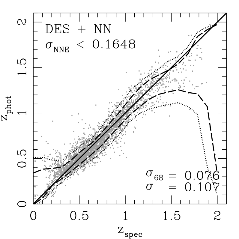
Figure 11.— $z_{\rm phot}$ vs $z_{\rm spec}$ for the DES catalog when the 10% of the objects with largest estimated NNE error (NNE error larger than 0.1648) have been removed. For comparison, see Figure 1.

Figure 11 shows $z_{\rm phot}$ vs. $z_{\rm spec}$ for the DES catalog with NN photo-z’s when 10% of the objects, those with the largest estimated NNE errors, have been removed. Comparing to the results in the upper panel of Fig. 1, this process reduces the photo-z scatter in the remaining objects by $\sim$ 23%. Moreover, most of the catastrophic objects at low redshift are removed, improving the bias and the scatter at those redshifts.

This procedure of removing catastrophic objects changes the selection function of the sample, which in turn changes the redshift distribution. When culling a catalog using an estimated error, one should carefully consider the effects of the reduced sample size as well as the change in the selection function of the objects to be analyzed. Recently, there has been promising work showing that, for the DES mock catalog, the accuracy of galaxy power spectrum measurement can be improved by culling high estimated error galaxies using the MDE estimator (Banerji et al., in prep). The study finds that the improvement in the photo-z scatter outweighs the reduced statistics of the resulting smaller sample of low photo-z error galaxies.

6. Conclusions

In this paper, we have introduced a new approach to estimating photometric redshift errors using a spectroscopic training set. We presented two implementations of the training-set approach, Kd-tree and Nearest Neighbor Error (NNE), and found that NNE is the best error estimator when a representative training set is available. Compared to the $\chi^{2}$ error and the MDE estimators, training-set based error estimators are less sensitive to systematic errors in magnitude error estimates. They incorporate both the bias and scatter of the photo-z’s, important features given the often substantial biases in photo-z estimates. Comparison of NNE and Kd-tree errors with error estimators from the literature shows that these training-set error estimators are in general more accurate and better behaved (in the sense that the error residual distribution is closer to a Gaussian).

Since a fully representative spectroscopic training set is not always available, we explored the impact on these error estimates of non-representative training sets. We found that this does not substantially degrade the accuracy of the training-set error estimates. In fact, we showed that even for training sets with very different magnitude and redshift distributions from the photometric sample, the training-set error estimates remain accurate at the 10% level.

Finally, we demonstrated that one can cull galaxies with large estimated errors from a sample and thereby significantly improve the overall scatter and bias of the photo-z estimates. Because the training-set error estimators are more accurate than other error estimators, and because the photo-z error residuals are nearly Gaussian distributed for these methods, culling objects using NNE or Kd-tree results in greater performance improvement than culling with other error estimators.

7. Acknowledgments

We would like to thank Erin Sheldon for insightful and useful discussions, as well as Dinoj Surendran and Mark SubbaRao for introducing the authors to a fast method of nearest neighbor search using Cover-Trees.

This work was supported in part by the Kavli Institute for Cosmological Physics at the University of Chicago through grants NSF PHY-0114422 and NSF PHY-0551142 and an endowment from the Kavli Foundation and its founder Fred Kavli. HO was additionally supported by the NSF grants AST-0239759, AST-0507666, and AST-0708154 at the University of Chicago. ML was additionally supported by the Department of Energy grant to the University of Chicago and Fermilab. Support for CC is made available through the contract between DOE and Fermi Research Alliance, LLC, contract number DE-AC02-07CH11359.

Funding for the SDSS and SDSS-II has been provided by the Alfred P. Sloan Foundation, the Participating Institutions, the National Science Foundation, the U.S. Department of Energy, the National Aeronautics and Space Administration, the Japanese Monbukagakusho, the Max Planck Society, and the Higher Education Funding Council for England. The SDSS Web Site is http://www.sdss.org/.

The SDSS is managed by the Astrophysical Research Consortium for the Participating Institutions. The Participating Institutions are the American Museum of Natural History, Astrophysical Institute Potsdam, University of Basel, University of Cambridge, Case Western Reserve University, University of Chicago, Drexel University, Fermilab, the Institute for Advanced Study, the Japan Participation Group, Johns Hopkins University, the Joint Institute for Nuclear Astrophysics, the Kavli Institute for Particle Astrophysics and Cosmology, the Korean Scientist Group, the Chinese Academy of Sciences (LAMOST), Los Alamos National Laboratory, the Max-Planck-Institute for Astronomy (MPIA), the Max-Planck-Institute for Astrophysics (MPA), New Mexico State University, Ohio State University, University of Pittsburgh, University of Portsmouth, Princeton University, the United States Naval Observatory, and the University of Washington.

References

- Abazajian et al. (2003) Abazajian, K. et al. 2003, AJ, 126, 2081
- Adelman-McCarthy et al. (2007) Adelman-McCarthy, J. K. et al. 2007, ArXiv e-prints, 707
- Avni (1976) Avni, Y. 1976, ApJ, 210, 642
- Baygelzimer et al. (2006) Baygelzimer, A., Kakade, S., & Langford, J. 2006, Proceedings of the 23rd International Conference on Machine Learning
- Benitez (2000) Benitez, N. 2000, ApJ, 536, 571
- Bishop (1995) Bishop, C. M. 1995, Neural Networks for Pattern Recognition (Oxford University Press)
- Bolzonella et al. (2000) Bolzonella, M., Miralles, J.-M., & Pelló, R. 2000, A&A, 363, 476
- Brunner et al. (1999) Brunner, R. J., Connolly, A. J., & Szalay, A. S. 1999, ApJ, 516, 563
- Bruzual & Charlot (1993) Bruzual, A. G. & Charlot, S. 1993, ApJ, 405, 538
- Capak et al. (2004) Capak, P., Cowie, L. L., Hu, E. M., Barger, A. J., Dickinson, M., Fernandez, E., Giavalisco, M., Komiyama, Y., Kretchmer, C., McNally, C., Miyazaki, S., Okamura, S., & Stern, D. 2004, AJ, 127, 180
- Coleman et al. (1980) Coleman, G. D., Wu, C. C., & Weedman, D. W. 1980, ApJS, 43, 393
- Collister & Lahav (2004) Collister, A. A. & Lahav, O. 2004, PASP, 116, 345
- Connolly et al. (1995) Connolly, A. J., Szalay, A. S., Bershady, M. A., Kinney, A. L., & Calzetti, D. 1995, AJ, 110, 1071
- Cowie et al. (2004) Cowie, L. L., Barger, A. J., Hu, E. M., Capak, P., & Songaila, A. 2004, AJ, 127, 3137
- Csabai et al. (2003) Csabai, I., Budavári, T., Connolly, A. J., Szalay, A. S., Győry, Z., Benítez, N., Annis, J., Brinkmann, J., Eisenstein, D., Fukugita, M., Gunn, J., Kent, S., Lupton, R., Nichol, R. C., & Stoughton, C. 2003, AJ, 125, 580
- Cunha et al. (2008) Cunha, C. et al. 2008, in prep
- Hsieh et al. (2005) Hsieh, B.-C., Yee, H. K. C., Lin, H., & Gladders, M. D. 2005
- Huterer et al. (2004) Huterer, D., Kim, A., Krauss, L. M., & Broderick, T. 2004, ApJ, 615, 595
- Huterer et al. (2006) Huterer, D., Takada, M., Bernstein, G., & Jain, B. 2006, MNRAS, 366, 101
- Lima & Hu (2007) Lima, M. & Hu, W. 2007, ArXiv e-prints, 709
- Lima et al. (2008) Lima, M. et al. 2008, in prep
- Lin et al. (1999) Lin, H., Yee, H. K. C., Carlberg, R. G., Morris, S. L., Sawicki, M., Patton, D. R., Wirth, G., & Shepherd, C. W. 1999, ApJ, 518, 533
- Ma et al. (2006) Ma, Z., Hu, W., & Huterer, D. 2006, ApJ, 636, 21
- Oyaizu et al. (2007) Oyaizu, H., Lima, M., Cunha, C. E., Lin, H., Frieman, J., & Sheldon, E. S. 2007, ArXiv e-prints, 708
- Poli et al. (2003) Poli, F., Giallongo, E., Fontana, A., Menci, N., Zamorani, G., Nonino, M., Saracco, P., Vanzella, E., Donnarumma, I., Salimbeni, S., Cimatti, A., Cristiani, S., Daddi, E., D’Odorico, S., Mignoli, M., Pozzetti, L., & Renzini, A. 2003, ApJ, 593, L1
- Press et al. (1992) Press, W. H., Teukolsky, S. A., Vetterling, W. T., & Flannery, B. P. 1992, Numerical recipes in C. The art of scientific computing (Cambridge: University Press, —c1992, 2nd ed.)
- Scranton et al. (2005) Scranton, R., Connolly, A. J., Szalay, A. S., Lupton, R. H., Johnston, D., Budavari, T., Brinkman, J., & Fukugita, M. 2005, ArXiv Astrophysics e-prints
- The Dark Energy Survey Collaboration (2005) The Dark Energy Survey Collaboration. 2005, ArXiv Astrophysics e-prints
- Wadadekar (2005) Wadadekar, Y. 2005, Publ. Astron. Soc. Pac., 117, 79
- Wirth et al. (2004) Wirth, G. D., Willmer, C. N. A., Amico, P., Chaffee, F. H., Goodrich, R. W., Kwok, S., Lyke, J. E., Mader, J. A., Tran, H. D., Barger, A. J., Cowie, L. L., Capak, P., Coil, A. L., Cooper, M. C., Conrad, A., Davis, M., Faber, S. M., Hu, E. M., Koo, D. C., Le Mignant, D., Newman, J. A., & Songaila, A. 2004, AJ, 127, 3121
- Zhan & Knox (2006) Zhan, H. & Knox, L. 2006, ApJ, 644, 663