Resonant Transmission of a Light Pulse through a Quantum Well

Аннотация

Reflectance, transmittance and absorbance of a symmetric light pulse, the carrying frequency of which is close to the frequency of interband transitions in a quantum well, are calculated. Energy levels of the quantum well are assumed discrete, and two closely located excited levels are taken into account. The theory is applicable for the quantum wells of arbitrary widths when the size quantization is preserved. A distinction of refraction indices of barriers and quantum well is taken into account. In such a case, some additional reflection from the quantum well borders appears which changes essentially a shape of the reflected pulse in comparison to homogeneous medium. The reflection from the borders disappears at some definite ratios of the carrying frequency of the stimulating pulse and quantum well width.

I Введение

The optical characteristics (reflectance, transmittance and absorbance) of a quantum well were calculated 1; 2; 3; 4 for a symmetric light pulse. A narrow quantum well with one excited energy level and a homogeneous medium (when the refraction indices of barriers $\nu_{1}$ and of a quantum well $\nu$ are equal) were considered 4. It was assumed in 2 that $\nu=\nu_{1}$ in a narrow quantum well (QW) with two closely located excited energy levels. A wide QW (the QW’s width is comparable with a light wave length corresponding to the carrying frequency of the light pulse) at $\nu=\nu_{1}$ is considered in 4. A wide QW with one excited energy level at $\nu\neq\nu_{1}$ is considered in 3. It was shown that the heterogeneous medium influenced essentially the shapes of the reflected and transmitted pulses. The reflected pulses undergo the greatest changes.

The present work is devoted to an investigation of the time and spatial dependencies of the reflectance and transmittance of a symmetrical light pulse going through a QW having a narrow doublet of the excited energy levels and under condition $\nu\neq\nu_{1}$. This question is of interest, since the relaxation processes of the system influence a distortion of the reflected and transmitted pulses and the correlation of lifetimes of two excited energy levels. In a homogeneous medium, the reflected pulse depends only on the resonance with the discrete energy levels of the QW. If $\nu\neq\nu_{1}$, an additional reflection from the QW borders appears. An interference of the additional contributions results in an unconventional dependance of the optical characteristics on the QW width.

It is assumed that the contributions of the radiative and nonradiative relaxation mechanisms may be comparable at low temperatures, low impurity doping and perfect QW boundaries. It means that one have to take into account all the orders on the electron - electromagnetic field interaction 5; 6; 7; 8; 9; 10; 11. The estimates 12 show that the preservation of the size quantized energy levels is possible at $kd\geq 1$ ($d$ is the QW width, $k$ is the module of the wave vector of the electromagnetic wave corresponding to the carrying frequency of the light pulse). In such a case one has to take into account a spatial dispersion of waves composing the light pulse12; 13; 14.

A system of a semiconductor QW of type I located in the interval $0\leq z\leq d$ and two semi-infinite barriers is considered. The system is situated in a constant quantizing magnetic field directed perpendicularly to the QW plane $xy$ and providing a discreteness of the energy levels. A stimulating light pulse propagates along the $z$ axis from the side of negative values $z$. The barriers are transparent for the light pulse which is absorbed in the quantum well to initiate the direct interband transitions. The intrinsic semiconductor and zero temperature are assumed.

The final results for two closely spaced energy levels of the electronic system in a quantum well are obtained. Effect of other levels on the optical characteristics may be neglected, if the carrying frequency $\omega_{\,\ell}$ of the light pulse is close to the frequencies $\omega_{1}$ and $\omega_{2}$ of the doublet levels, and other energy levels are fairly distant. It is assumed that the doublet is situated near the minimum of the conduction band, the energy levels may be considered in the effective mass approximation, and the barriers are infinitely high. In particular, the narrow doublet may be realized by a magnetopolaron state 14.

II The Fourier-transforms of electric fields of transmitted and reflected pulses

Let us consider a situation when a symmetric exciting light pulse of a circular polarization propagates through a single quantum well along the $z$ axis from the side of negative values of $z$. Its electric field is as follows

$$\bf{E}_{0}(z,t)\leavevmode\nobreak\ = \leavevmode\nobreak\ \bf{e}_{\ell}E_{0}(z,t)\leavevmode\nobreak\ +\leavevmode\nobreak\ c.c.,$$

$$E_{0}(z,t)\leavevmode\nobreak\ = \leavevmode\nobreak\ E_{0}e^{-i\omega_{\ell}\,p}\Big{\{}\Theta(p)e^{-\gamma_{\ell}\,p/2}$$ (1)

$$+ [1-\Theta(p)]e^{\gamma_{\ell}p/2}\Big{\}}.$$

Here $E_{0}$ is the real amplitude, $p=t-\nu_{1}z/c,\leavevmode\nobreak\ \bf{e}_{\ell}=(\bf{e}_{x}\pm i\bf{e}_{y})/\sqrt{2}$ is the circular polarization vector, $\bf{e}_{x}$ и $\bf{e}_{y}$ are the real unite vectors, $\Theta(p)$ is the Heaviside function, $\omega_{\ell}$ is the carrying frequency of the light pulse, $\gamma_{\ell}$ is the pulse broadening, $c$ is the light velocity in vacuum. The Fourier-transform of (II) is

$$\bf{E}_{0}(z,\omega)=[\bf{e}_{\ell}E_{0}(\omega)+\bf{e}_{\ell}^{*}E_{0}(-\omega)]e^{ik_{1}z},$$

$$E_{0}(\omega)=\frac{E_{0}\leavevmode\nobreak\ \gamma_{\ell}}{(\omega-\omega_{\ell})^{2}+(\gamma_{\ell}/2)^{2}},\leavevmode\nobreak\ \leavevmode\nobreak\ \leavevmode\nobreak\ \leavevmode\nobreak\ k_{1}=\frac{\nu_{1}\omega}{c}.$$ (2)

The electric field at $z\leq 0$ is a sum of the electric fields of the stimulating and reflected pulses. Its Fourier-transform may be represented as

$$\bf{E}^{\ell}(z,\omega)=\bf{E}_{0}(z,\omega)+\Delta\bf{E}^{\ell}(z,\omega),$$

where $\Delta\bf{E}^{\ell}(z,\omega)$ is the electric field of the reflected pulse

$$\Delta\bf{E}^{\ell}(z,\omega)=\bf{e}_{\ell}\Delta E^{\ell}(z,\omega)+\bf{e}_{\ell}^{*}\Delta E^{\ell}(z,-\omega).$$ (3)

The transmitted pulse propagates in the region $z\geq d$. Its Fourier-transform is

$$\bf{E}^{r}(z,\omega)=\bf{e}_{\ell}E^{r}(z,\omega)+\bf{e}_{\ell}^{*}E^{r}(z,-\omega).$$ (4)

The functions $\Delta E^{\ell}(z,\omega)$ and $E^{r}(z,\omega)$ may be considered as the scalar amplitudes of monochromatic waves appearing as a result of the exciting monochromatic wave propagation through the QW. The similar problem has been solved in the case when the interaction of the electronic system with the electromagnetic wave could not be considered as a weak perturbation, as well as at $kd\neq 0$ and $\nu\neq\nu_{1}$ and there were two closely located excited energy levels 15.

It has been shown that

$$\Delta E^{\ell}(z,\omega)=\mathcal{C}_{R}e^{-ik_{1}z},\leavevmode\nobreak\ \leavevmode\nobreak\ \leavevmode\nobreak\ \leavevmode\nobreak\ z\leq 0,$$ (5)

$$E^{r}(z,\omega)=\mathcal{C}_{T}e^{ik_{1}z},\leavevmode\nobreak\ \leavevmode\nobreak\ \leavevmode\nobreak\ z\geq d,$$ (6)

$\mathcal{C}_{R}$ and $\mathcal{C}_{T}$ determine the amplitudes of reflected and transmitted waves, respectively. The following expressions for them are obtained

$$\mathcal{C}_{R} = E_{0}{\rho\over\Delta},$$

$$\mathcal{C}_{T} = 4E_{0}\zeta{1+(-1)^{m_{c}+m_{v}}e^{-ikd}N\over\Delta}e^{-ik_{1}d},$$ (7)

$$\Delta=L-2(\zeta-1)\big{[}(\zeta+1)e^{-ikd}+(-1)^{m_{c}+m_{v}}(\zeta-1)\big{]}N,$$ (8)

$$\rho = 2i(\zeta^{2}-1)\sin(kd)+2\big{[}(\zeta^{2}+1)e^{-ikd}$$ (9)

$$+ (-1)^{m_{c}+m_{v}}(\zeta^{2}-1)\big{]}N.$$

In (II) - (9) we used the designations

$$\zeta = k/k_{1}=\nu/\nu_{1},\leavevmode\nobreak\ \leavevmode\nobreak\ \leavevmode\nobreak\ k=\nu\omega/c,$$

$$L = (\zeta+1)^{2}e^{-ikd}-(\zeta-1)^{2}e^{ikd},$$ (10)

$m_{c}(m_{v})$ is the electron (hole) quantum number of the size quantization. It was assumed that one pair of numbers $m_{c},m_{v}$ corresponded to two direct interband transitions.

The dependance on the variable $\omega$ is determined by the function $N$

$$N=\frac{-i(-1)^{m_{c}+m_{v}}\leavevmode\nobreak\ (\varepsilon^{\prime}/2)\leavevmode\nobreak\ \Omega_{0}\leavevmode\nobreak\ e^{ikd}}{\tilde{\omega}_{1}\tilde{\omega}_{2}+i(\varepsilon/2)\leavevmode\nobreak\ \Omega_{0}}.$$ (11)

The designations

$$\Omega_{0} = \gamma_{r1}\tilde{\omega}_{2}+\gamma_{r2}\tilde{\omega}_{1},$$

$$\tilde{\omega}_{j} = \omega-\omega_{j}+i\gamma_{j}/2,\leavevmode\nobreak\ \leavevmode\nobreak\ \leavevmode\nobreak\ \tilde{\gamma}_{rj}=\varepsilon^{\prime}\gamma_{rj},\leavevmode\nobreak\ \leavevmode\nobreak\ \leavevmode\nobreak\ j=1,2.$$ (12)

are introduced in (11). Here $\omega_{j}$ are the frequencies of interband transitions on the doublet energy levels , $\gamma_{j}$ and $\gamma_{rj}\sim e^{2}/(\hbar c\,\nu)$ are the radiative and nonradiative broadenings of the doublet levels 14.

The function $N$ contains the complex value $\varepsilon=\varepsilon^{\prime}+i\varepsilon^{\prime\prime}$ 3; 13; 15

$$\varepsilon=\int_{0}^{d}dz\Phi(z)\Bigg{\{}\int_{0}^{z}dye^{ik(z-y)}\Phi(y)+\int_{z}^{d}dye^{ik(y-z)}\Phi(y)\Bigg{\}}.$$ (13)

It determines the influence of the spatial dispersion on the radiative broadening $\varepsilon^{\prime}\gamma_{rj}$ and shift $\varepsilon^{\prime\prime}\gamma_{rj}$ of the doublet levels.

Realizing a derivation of (13) we assumed the Lorentz force determined by the external magnetic field exceeded the Coulomb and exchange forces inside of the electron-hole pair, and the dependance of the wave function of the electron-hole pair may be represented by the factor $\Phi(z)$ 15.

III The time dependance of the electric field of reflected and transmitted light pulses

The time dependance of the amplitudes $E^{\ell}(z,\omega)$ and $E^{r}(z,\omega)$ is determined by well known formulas

$$\Delta E^{\ell}(z,t) \equiv \Delta E^{\ell}(s)=\frac{1}{2\pi}\int_{-\infty}^{+\infty}d\omega e^{-i\omega\,s}\Delta E^{\ell}(z,\omega),$$

$$s = t+\nu_{1}z/c,$$ (14)

$$E^{r}(z,t) \equiv E^{r}(p)=\frac{1}{2\pi}\int_{-\infty}^{+\infty}d\omega e^{-i\omega\,p}E^{r}(z,\omega),$$

$$p = t-\nu_{1}z/c.$$ (15)

It is seen from (II) and (8) that the amplitudes $\Delta E^{\ell}(z,\omega)$ and $E^{r}(z,\omega)$ have the identical denominators and, accordingly, identical poles on the complex plane $\omega$. Having used (II), (II)-(9) and (11), we obtain the electric fields in the integral form:

$$E^{r}(p)=\frac{2\zeta E_{0}\,\gamma_{\ell}\exp(-ik_{1}d)}{\pi L}\int_{-\infty}^{+\infty}d\omega$$

$$\times\frac{U(\omega)\exp(-i\omega p)}{[(\omega-\omega_{\ell})^{\,2}+(\gamma_{\ell}/2)^{\,2}](\omega-\Omega_{1})\,(\omega-\Omega_{2})},$$ (16)

$$\Delta E^{\ell}(s)=\frac{E_{0}\,\gamma_{\ell}}{2\pi L}\int_{-\infty}^{+\infty}d\omega$$

$$\times\frac{V(\omega)\exp(-i\omega s)}{[(\omega-\omega_{\ell})^{\,2}+(\gamma_{\ell}/2)^{\,2}](\omega-\Omega_{1})\,(\omega-\Omega_{2})},$$ (17)

where

$$U(\omega)=\tilde{\omega}_{1}\,\tilde{\omega}_{2}-\varepsilon^{\prime\prime}\,\Omega_{0}/2,$$ (18)

$$V(\omega)=a\,\tilde{\omega}_{1}\,\tilde{\omega}_{2}+A\,\Omega_{0}/2.$$ (19)

The designations

$$a=2i(\zeta^{2}-1)\sin(kd),$$ (20)

$$A=ia\,\varepsilon-2i(-1)^{m_{c}+m_{v}}[\zeta^{2}+1+(-1)^{m_{c}+m_{v}}(\zeta^{2}-1)]\,\varepsilon^{\prime}$$ (21)

are introduced in (19). The denominators of integrands of (III) and (III) have four identical poles on the complex plane $\omega$: $\omega=\omega_{\ell}\pm i\gamma_{\ell}/2,\,\omega=\Omega_{1},\,\omega=\Omega_{2}$. The pole in the upper semi-plane $\omega=\omega_{\ell}+i\gamma_{\ell}/2$ defines the time dependance at $p(s)\leq 0$, three remainder poles are at $p(s)\geq 0$. The poles $\Omega_{1}$ and $\Omega_{2}$ have the view

$$\Omega_{1(2)}={1\over 2}\bigg{\{}\omega_{1}+\omega_{2}-(i/2)\,[\gamma_{1}+\gamma_{2}+f(\gamma_{r1}+\gamma_{r2})]$$

$$\pm\Big{[}\big{\{}\omega_{1}-\omega_{2}-(i/2)\,[\gamma_{1}-\gamma_{2}+f(\gamma_{r1}-\gamma_{r2})]\big{\}}^{2}$$

$$-f^{2}\gamma_{r1}\gamma_{r2}\Big{]}^{1/2}\bigg{\}}.$$ (22)

The complex coefficient $f=f_{2}+if_{1}$ enters in $\Omega_{1}$ and $\Omega_{2}$ as combinations $f\,\gamma_{r1}$ and $f\,\gamma_{r2}$,

$$f_{1}=\varepsilon^{\prime\prime}-\frac{(-1)^{m_{c}+m_{v}}\varepsilon^{\prime}(1-\zeta^{2})\sin kd}{1+\zeta^{2}+(-1)^{m_{c}+m_{v}}(1-\zeta^{2})\cos kd},$$ (23)

$$f_{2}=\frac{2\varepsilon^{\prime}\zeta}{1+\zeta^{2}+(-1)^{m_{c}+m_{v}}(1-\zeta^{2})\cos kd}.$$ (24)

The mentioned above four poles determine the resonant contributions at the integration of (III) and (III). There are a row of poles connected with nulls of the function $L$, situated on the lower semi-plane $\omega$. However, these poles are located far away of the real axis, Однако эти полюсы расположены далеко от вещественной оси, and their contributions may be neglected in comparison with the resonant terms.

The time dependance of the electric fields may be represented as

$$E^{r}(p) = (4\zeta E_{0}/L)\{[1-\Theta(p)]J_{1}$$

$$+ (J_{2}+J_{3}+J_{4})\Theta(p)\}\exp(-ik_{1}d),$$

$$\Delta E^{\ell}(s) = (E_{0}/L)\{[1-\Theta(s)]K_{1}+(K_{2}$$ (25)

$$+ K_{3}+K_{4})\Theta(s)\},$$

where

$$J_{1(2)}=\frac{U(\omega_{\ell}\pm i\gamma_{\ell}/2)\exp[-i(\omega_{\ell}\pm i\gamma_{\ell}/2)\,p\,]}{(\omega_{\ell}-\Omega_{1}\pm i\gamma_{\ell}/2)\,(\omega_{\ell}-\Omega_{2}\pm i\gamma_{\ell}/2)},$$ (26)

$$J_{3(4)}=\mp\frac{i\gamma_{\ell}U(\Omega_{1(2)})\exp(-i\Omega_{1(2)}\,p)}{(\Omega_{1}-\Omega_{2})\,[(\omega_{\ell}-\Omega_{1(2)})^{\,2}+(\gamma_{\ell}/2)^{\,2}]}$$ (27)

$$K_{1(2)}=\frac{V(\omega_{\ell}\pm i\gamma_{\ell}/2)\exp[-i(\omega_{\ell}\pm i\gamma_{\ell}/2)\,s\,]}{(\omega_{\ell}-\Omega_{1}\pm i\gamma_{\ell}/2)\,(\omega_{\ell}-\Omega_{2}\pm i\gamma_{\ell}/2)},$$ (28)

$$K_{3(4)}=\mp\frac{i\gamma_{\ell}\,V(\Omega_{1(2)})\exp(-i\Omega_{1(2)}\,s)}{(\Omega_{1}-\Omega_{2})\,[(\omega_{\ell}-\Omega_{1(2)})^{\,2}+(\gamma_{\ell}/2)^{\,2}]}.$$ (29)

After the substitutions $\tilde{\omega}_{1},\tilde{\omega}_{2}$ and $\Omega_{0}$, the functions $U(\omega)$ and $V(\omega)$ have the form

$$U(\omega)=(\omega-\omega_{1}+i\gamma_{1}/2)(\omega-\omega_{2}+i\gamma_{2}/2)-(\varepsilon^{\prime\prime}/2)$$

$$\times[\gamma_{r1}(\omega-\omega_{2}+i\gamma_{2}/2)+\gamma_{r2}(\omega-\omega_{1}+i\gamma_{1}/2)],$$ (30)

$$V(\omega)=a\,(\omega-\omega_{1}+i\gamma_{1}/2)(\omega-\omega_{2}+i\gamma_{2}/2)+(A/2)$$

$$\times[\gamma_{r1}(\omega-\omega_{2}+i\gamma_{2}/2)+\gamma_{r2}(\omega-\omega_{1}+i\gamma_{1}/2)].$$ (31)

Obtaining (III) для $\Omega_{1}$, $\Omega_{2}$ we assumed that $\omega_{\ell}$ was close to the resonant frequencies $\omega_{1}$ and $\omega_{2}$. Therefore the parameters $k$ and $k_{1}$ are $k=\nu\omega_{\ell}/c,\leavevmode\nobreak\ \leavevmode\nobreak\ \leavevmode\nobreak\ k_{1}=\nu_{1}\omega_{\ell}/c$. The analogical approximation was used in 3.

IV Extreme cases

It follows from (III) and (III) that $\Delta E^{\ell}(s)$ may be represented as a sum of two summands which are proportional to $a$ and $A$, respectively. The coefficient $a$ equals 0 in two extreme cases: if $\zeta=1$ (the homogeneous medium approximation), or $kd=0$ (a narrow QW). The second summand equals 0, if $\gamma_{r1}=\gamma_{r2}=0$. Hence, one may conclude that the first summand is stipulated by reflection from the QW boundaries, and the second by the resonance with the QW energy levels.

It is seen from (13), (23) and(24) that in the case $kd=0\leavevmode\nobreak\ \varepsilon^{\prime\prime}=f_{1}=0,\leavevmode\nobreak\ \varepsilon^{\prime}=1,f_{2}=\zeta$ (if $m_{c}+m_{v}$ is an even number) and $f_{2}=1/\zeta$  ($m_{c}+m_{v}$ is an odd number). Thus, in such case $\gamma_{r1}$ и $\gamma_{r21}$ are renormalized by the factor $\zeta$ (or $\zeta^{-1}$), and in the rest the formulas for the fields coincide with the formulas obtained in 2. If $\zeta=1,\leavevmode\nobreak\ kd\neq 0$, (III) and (III) pass into the formulas obtained in 4.

Below a calculation is being provided for the case

$$\gamma_{r1}=\gamma_{r2}=\gamma_{r},\leavevmode\nobreak\ \leavevmode\nobreak\ \gamma_{1}=\gamma_{2}=\gamma.$$

Such equality is possible, for instance, if the doublet is formed by a magnetopolaron when the cyclotron frequency is equal to the longitudinal optical phonon frequency 14. In such limiting case $\Omega_{1(2)}$ (III) equal:

$$\Omega_{01(2)}={1\over 2}\bigg{[}\omega_{1}+\omega_{2}-i(\gamma+f\gamma_{r})\pm\sqrt{(\omega_{1}-\omega_{2})^{2}-f^{2}\gamma_{r}^{2}}\leavevmode\nobreak\ \bigg{]}.$$ (32)

For an homogeneous medium $(\zeta=1)$ it follows from (23) and (24) that $f=\varepsilon$ and $\Omega_{01(2)}$ coincides with the analogical formulas from 4. Thus, a transition to a heterogeneous medium leads to the replacement in the resonant denominators in formulas (26) - (29) the function $\varepsilon$ by the coefficient $f$ which influences now the shift $f_{1}$ and the radiative broadening $f_{2}$ of the doublet energy levels. The analogical situation, as it is seen from (III), takes place and in the general case $\gamma_{r1}\neq\gamma_{r2},\gamma_{r}\neq\gamma_{r}$.

For the sake of convenience of numerical calculations, let us go to the new variables

$$\Omega = \omega_{\ell}-\omega_{1},\leavevmode\nobreak\ \leavevmode\nobreak\ \Delta\omega=\omega_{1}-\omega_{2},\leavevmode\nobreak\ \leavevmode\nobreak\ \beta_{01}=\Omega_{01}-\omega_{1},$$

$$\beta_{02} = \Omega_{02}-\omega_{1},$$ (33)

(with the help of these variables the number of the independent parameters in expressions for optical characteristics diminishes on one), and to introduce also the resonant frequency

$$\Omega_{res}\equiv Re\leavevmode\nobreak\ \beta_{01}={1\over 2}\bigg{[}-\Delta\omega+f_{1}\gamma_{r}+Re\leavevmode\nobreak\ \sqrt{\Delta\omega^{2}-f^{2}\gamma_{r}^{2}}\leavevmode\nobreak\ \bigg{]},$$ (34)

corresponding to the interband resonant transition with the frequency $\omega_{1}$, renormalized by the radiative shift.

In this extreme case, the electric fields take the form

$$E^{r}(p) = (4\zeta E_{0}/L)e^{-i(k_{1}d+\omega_{\ell}p)}\{[1-\Theta(p)\,]J_{01}$$

$$+ (J_{02}+J_{03}+J_{04})\Theta(p)\},$$

$$\Delta E^{\ell}(s) = (4E_{0}/L)e^{-i\omega_{\ell}s}\{[1-\Theta(s)]K_{01}$$ (35)

$$+ (K_{02}+K_{03}+K_{04})\Theta(s)\},$$

$$J_{01(2)}=\frac{\exp(\pm\gamma_{\ell}\,p/2)\leavevmode\nobreak\ U_{0}(\Omega\pm i\gamma_{\ell}/2)}{(\Omega-\beta_{01}\pm i\gamma_{\ell}/2)\,(\Omega-\beta_{02}\pm i\gamma_{\ell}/2)},$$ (36)

$$J_{03(4)}=\mp\frac{i\gamma_{\ell}\exp[i(\Omega-\beta_{01(2)})\,p\,]\leavevmode\nobreak\ U_{0}(\Omega_{01(2)})}{\sqrt{\Delta\omega^{2}-f^{2}\gamma_{r}^{2}}\leavevmode\nobreak\ [(\Omega-\beta_{01(2)})^{\,2}+(\gamma_{\ell}/2)^{\,2}\,]\,},$$ (37)

$$K_{01(2)}=\frac{\exp(\pm\gamma_{\ell}\,s/2)\leavevmode\nobreak\ V_{0}(\Omega\pm i\gamma_{\ell}/2)}{(\Omega-\beta_{01}\pm i\gamma_{\ell}/2)\,(\Omega-\beta_{02}\pm i\gamma_{\ell}/2)},$$ (38)

$$K_{03(4)}=\mp\frac{i\gamma_{\ell}\exp[i(\Omega-\beta_{01(2)})\,s\,]\leavevmode\nobreak\ V_{0}(\Omega_{01(2)})}{\sqrt{\Delta\omega^{2}-f^{2}\gamma_{r}^{2}}\leavevmode\nobreak\ [(\Omega-\beta_{01(2)})^{2}+(\gamma_{\ell}/2)^{2}\,]}.$$ (39)

Instead of (III) and (III) the functions

$$U_{0}(\omega) = (\omega+i\gamma/2)(2\omega+\Delta\omega+i\gamma)$$ (40)

$$- (\varepsilon^{\prime\prime}\gamma_{r}/2)(2\omega+\Delta\omega+i\gamma),$$

$$V_{0}(\omega) = a(\omega+i\gamma/2)\,(\omega+\Delta\omega+i\gamma/2)$$ (41)

$$+ (A\leavevmode\nobreak\ \gamma_{r}/2)(2\omega+\Delta\omega+i\gamma),$$

appear, where $a$ and $A$ are determined in (20), (21).

It is of interest a case when $\gamma_{r1}=\gamma_{r2}=0$,i.e., the interaction of the electromagnetic waves with the electronic system is absent. It may happen for the frequencies faraway from the resonance when the absorption is neglected. In such a case it follows from (III) - (III) that

$$E^{r}(p)=(4\zeta/L)E_{0}(z,t),\leavevmode\nobreak\ \leavevmode\nobreak\ \leavevmode\nobreak\ \Delta E^{\ell}(s)=(a/L)E_{0}(z,t),$$ (42)

where $E_{0}(z,t)$ is the scalar amplitude of the field of the exciting pulse (II). Thus, for an transparent QW the electric fields of transmitted and reflected pulses are proportional to the field of the exciting pulse. The corresponding coefficients depend on $\zeta$ and $kd$.

V Reflection, transition and absorption of the exciting pulse

The energy flux $\bf{S}(p)$, corresponding to the electric field of the exciting pulse, is defined as 13

$$\bf{S}(p)=(\bf{e}_{z}/4\pi)(c\,\nu_{1})(\bf{E}_{0}(z,t))^{2}=\bf{e}_{z}S_{0}\mathcal{P}(p),$$ (43)

where $S_{0}=c\nu_{1}E_{0}^{2}/(2\pi)$, $\bf{e}_{z}$ is the unite vector along the axes $z$. The dimensionless function $\mathcal{P}(p)$ determines the spatial and time dependencies of the energy flux of the exciting pulse,

$$\mathcal{P}(p)={(\bf{E}_{0}(z,t))^{2}\over S_{0}}=\Theta(p)e^{-\gamma_{\ell}p}+[1-\Theta(p)]e^{\gamma_{\ell}p}.$$ (44)

Transmitted (on the right of the QW) and reflected (on the left of the QW) fluxes are determined as

$$\bf{S}^{r}(z,t)={\bf{e}_{z}\over 4\pi}c\nu_{1}(\bf{E}^{r}(z,t))^{2}=\bf{e}_{z}S_{0}\mathcal{T}(p),$$

$$\bf{S}^{\ell}(z,t)=-{\bf{e}_{z}\over 4\pi}c\nu_{1}(\Delta\bf{E}^{\ell}(z,t))^{2}=-\bf{e}_{z}S_{0}{\mathcal{R}}(s),$$ (45)

dimensionless functions $\mathcal{T}(p)$ and $\mathcal{R}(s)$ determine the parts of the transmitted and reflected energy of the stimulating pulse. The energy part $\mathcal{A}(t)$, concentrated inside of the QW, is being absorbed or irradiated again. It is defined by the obvious expression

$$\mathcal{A}(p)=\mathcal{P}(p)-\mathcal{R}(p)-\mathcal{T}(p)$$ (46)

(since for reflection $z\leq 0$, the variable in $\mathcal{R}$ is $s=t-|z|\nu/c$).

In the limiting case $\gamma_{r1}=\gamma_{r2}=\gamma_{r}\leavevmode\nobreak\ \leavevmode\nobreak\ \mathcal{A}=0,\,\mathcal{T}=|4\zeta/L|^{2}\mathcal{P}(t)$, $\mathcal{R}=|a/L|^{2}\mathcal{P}(t)$, where $P(t)$ corresponds to the stimulating pulse. Taking into account (II) we obtain

$$\mathcal{R}(t)=\frac{(\zeta^{2}-1)^{2}\sin^{2}(kd)}{4\zeta^{2}\cos^{2}(kd)+(\zeta^{2}+1)^{2}\sin^{2}(kd)}\mathcal{P}(t),$$

$$\mathcal{T}(t)=\frac{4\zeta^{2}}{4\zeta^{2}\cos^{2}(kd)+(\zeta^{2}+1)^{2}\sin^{2}(kd)}\mathcal{P}(t).$$ (47)

Thus, in this limiting case $\mathcal{R}$ is the reflectance of a transparent plate and equals 0 at $kd=0,\pi,2\pi...$.

For the calculations one has to define the function $\Phi(z)$, from the definition of $\varepsilon$ (13). $\Phi(z)$ was chosen as

$$\Phi(z)=(2/d)\sin(\pi m_{c}z/d)\sin(\pi m_{v}z/d),\leavevmode\nobreak\ \leavevmode\nobreak\ \leavevmode\nobreak\ \leavevmode\nobreak\ 0\leq z\leq d$$

and $\Phi(z)=0$ in the barriers, what corresponds to the free electron-hole pair. In the case of chosen above $\Phi(z)\leavevmode\nobreak\ \varepsilon^{\prime}$ and $\varepsilon^{\prime\prime}$, according to (13), are equal

$$\varepsilon^{\prime}=2\mathcal{B}^{2}[1-(-1)^{m_{c}+m_{v}}\cos(kd)],$$

$$\varepsilon^{\prime\prime}=2\mathcal{B}\Big{(}\frac{(1+\delta_{m_{c}+m_{v}})(m_{c}+m_{v})^{2}+(m_{c}-m_{v})^{2}}{8m_{c}m_{v}}$$

$$-(-1)^{m_{c}+m_{v}}\mathcal{B}\sin kd-\frac{(2+\delta_{m_{c}+m_{v}})(kd)^{2}}{8\pi^{2}m_{c}m_{v}}\Big{)},$$ (48)

$$\mathcal{B}=\frac{4\pi^{2}m_{c}m_{v}kd}{[\pi^{2}(m_{c}+m_{v})^{2}-(kd)^{2}]\,[(kd)^{2}-\pi^{2}(m_{c}-m_{v})^{2}]}$$

VI Calculation results and discussion

The poles $\Omega_{1}$ and $\Omega_{2}$ (III) determine the resonant frequencies $Re\leavevmode\nobreak\ \Omega_{1,2}$ and shift $Im\leavevmode\nobreak\ \Omega_{1,2}$ of the doublet levels. In the limiting case of a homogeneous medium and a narrow QW $\Omega_{1,2}$ coincide with values $(\Omega-iG/2)_{1(2)}$ obtained in 2. The broadenings $\gamma_{ri}$ of the doublet levels enter into electric fields of the pulse as $\varepsilon^{\prime}\,\gamma_{ri}$ and $\varepsilon^{\prime\prime}\gamma_{ri}$. In the cases of the monochromatic and pulse irradiation in a homogeneous medium $\varepsilon^{\prime}\,\gamma_{ri}$ and $\varepsilon^{\prime\prime}\,\gamma_{ri}$ determine the broadening and shift of the doublet levels 13; 15; 4. In the considered above general case of the pulse irradiation and heterogeneous medium, $\Omega_{1}$ and $\Omega_{2}$ contain $f_{1}\gamma_{ri}$ and $f_{2}\gamma_{ri}$ which depend on parameters $kd$ and $\zeta$ and on $\varepsilon^{\prime}\,\gamma_{ri}$ and $\varepsilon^{\prime\prime}\,\gamma_{ri}$. Thus, the view of functions $f_{2}$ and $f_{1}$ influence the radiative shift and broadening of the energy levels.

If $\zeta=1,kd\neq 0$, then $f_{1}=\varepsilon^{\prime\prime},f_{2}=\varepsilon^{\prime}$. In the case $kd=0$ the level shift is absent, and the broadening is determined by values $\zeta\gamma_{ri}$. Since at $kd\neq 0\leavevmode\nobreak\ \leavevmode\nobreak\ \gamma_{ri}\sim\nu^{-1}$, then $\zeta\gamma_{ri}\sim\nu_{1}^{-1}$ and is some broadening at zero width of a QW 15.

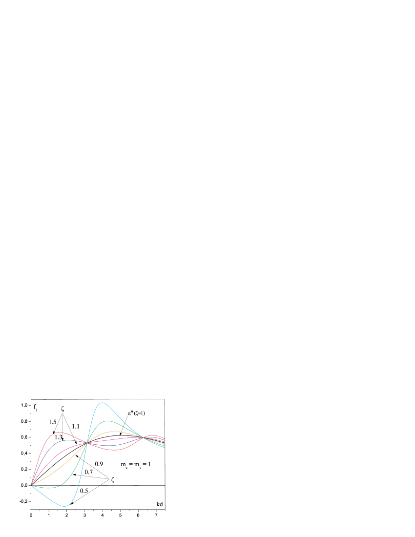
Рис. 1: $f_{1}$ as function of $kd$ (23)) at different values $\zeta=\nu/\nu_{1}$.

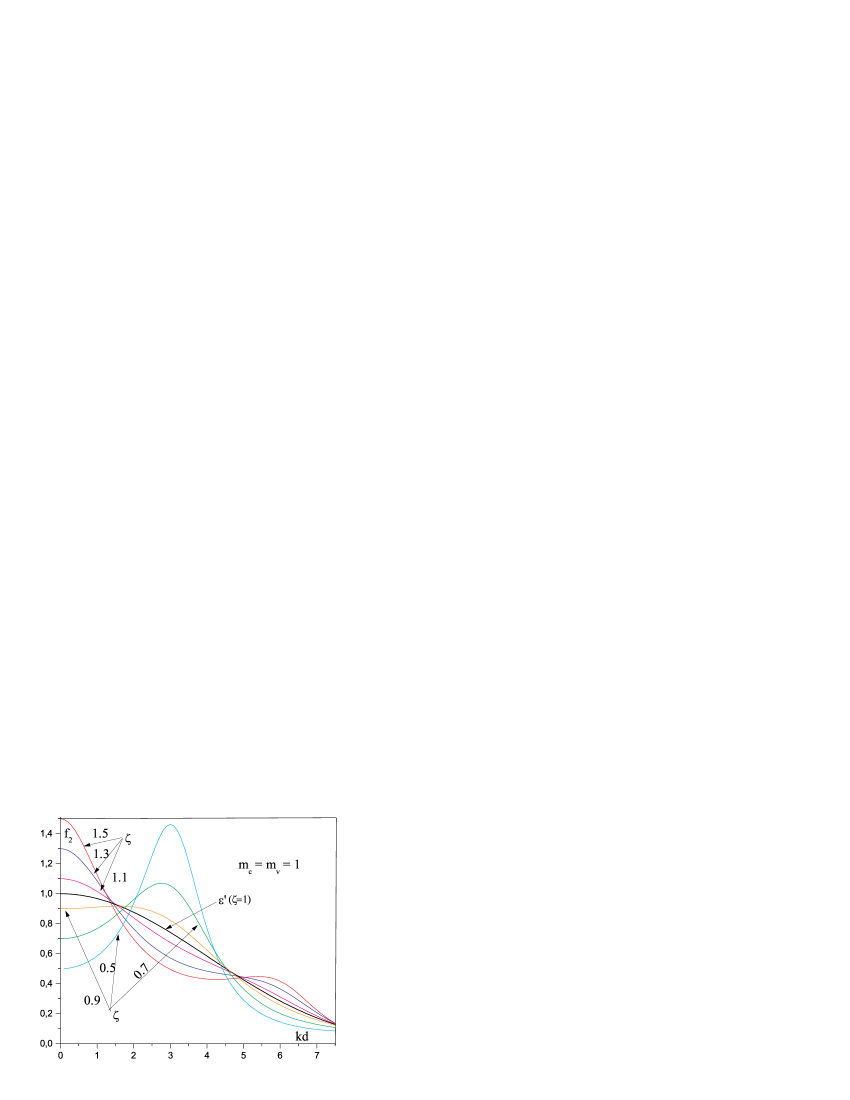
Рис. 2: $f_{2}$ as function of $kd$ (24) at different values $\zeta=\nu/\nu_{1}$.

In Fig.1 $f_{1}$ from (23) (which is connected with the shift of the doublet energy levels) is represented as a function of $kd$ for different values $\zeta$. It is seen that $f_{1}=\varepsilon^{\prime\prime}$ in the points $kd=0,\pi,2\pi...$, i.e.,the influence of the heterogeneous medium on the level shift disappears. $f_{2}$ ((24)) as a function of $kd$ is represented in Fig.2. The largest deviation $f_{2}$ from $\varepsilon^{\prime}$ takes place in the points $kd=0,\pi,2\pi...f_{2}$, since in these points $f_{2}=\zeta$.

The functions $\mathcal{R},\mathcal{A}$ and $\mathcal{T}$ were calculated for $\gamma_{r1}=\gamma_{r2}=\gamma_{r}$,  $\gamma_{1}=\gamma_{2}=\gamma$ according to (IV). It was assumed the direct interband transition with the quantum numbers $m_{c}=m_{v}=1$. It is shown in figures changes in time of the optical characteristics of a QW at passing of a light pulse for different values of parameters $kd$ and $\zeta=\nu/\nu_{1}$. Since the functions $\mathcal{R}$ and $\mathcal{T}$ are the homogeneous functions of the broadenings and of frequencies $\omega_{1},\omega_{2},\omega_{\ell}$, then the choice of the measuring units is unconditioned. All the values are expressed in $eV$ for the sake of certainty. All the curves $\mathcal{R,\mathcal{T}}$ and $\mathcal{A}$ are obtained for the case $\Omega=\Omega_{res}$, where   $\Omega$ and $\Omega_{res}$ are determined by the formulas (IV), (34).

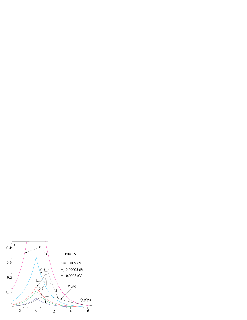
Рис. 3: The reflectance $\mathcal{R}$ as a function of time for a narrow (in comparison to $\Delta\omega$) stimulating pulse $(\Delta\omega=0.0065\leavevmode\nobreak\ eV)$ and small radiative broadening $\gamma_{r}\ll\gamma,\gamma_{\ell}$.

The reflectance $\mathcal{R}$ for an narrow in comparison with $\Delta\omega$ stimulating pulse and a small radiative broadening $(\gamma_{r}\ll\gamma,\gamma_{\ell})$ is represented in Fig.3. All the curves correspond to the value kd=1.5. In such a case, as it follows from Fig.1,2, the radiative broadening is close $\varepsilon^{\prime}\gamma_{r}$ and weakly dependant on $\zeta$. On the other hand, the radiative shift of energy levels $f_{1}=\varepsilon^{\prime\prime}-(1-\zeta^{2})/(1+\zeta^{2})$ depends substantially on the parameter $\zeta$. It is seen that the reflectance changes radically for an homogeneous medium $(\zeta=1)$ in comparison with a heterogeneous medium $(\zeta\neq 1)$. For instance, at $\zeta=1.3$ the reflectance in maximum increases 25 times in comparison with the case of $\zeta=1$, at $\zeta=0.7$ - 50 times. The sharp increasing of $\mathcal{R}$ is a manifestation of light reflection from the QW borders which equals 0 at $\zeta=1$.

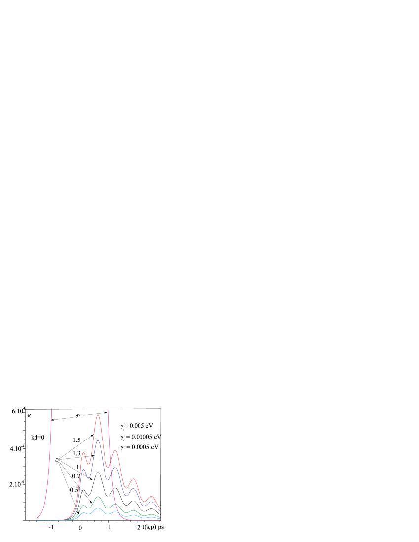
Рис. 4: The time dependance of the reflectance $\mathcal{R}$ for an exciting pulse of a middle duration $(\Delta\omega=0.0065eV,\gamma_{\ell}=0.005eV)$. The reflection from the QW borders is absent $(kd=0)$.

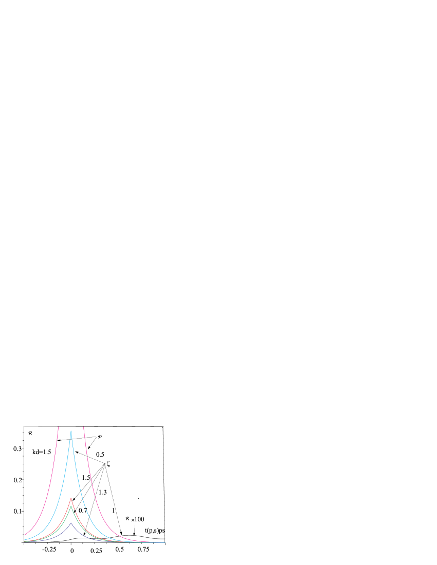
Рис. 5: The time dependance of the reflectance $\mathcal{R}$ for an exciting pulse of a middle duration $(\Delta\omega=0.0065eV,\gamma_{\ell}=0.005eV)$. The reflection from the QW borders is maximal $(kd=1.5)$.

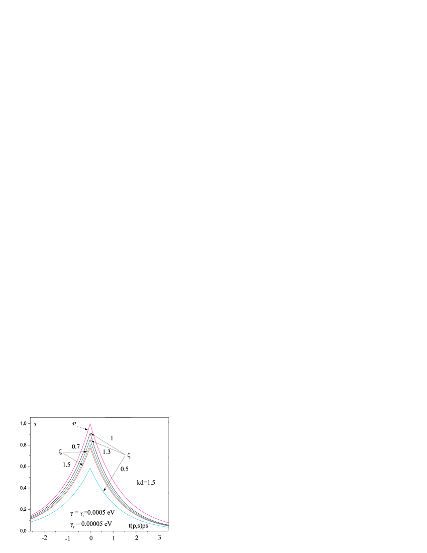
Рис. 6: The transmittance $\mathcal{T}$ in the case of maximal reflection from the QW borders $(kd=1.5)$. The parameters are the same as in Fig.4, 5.

An analogical situation is shown in Fig.4,5, which demonstrate a case of a light pulse of a middle duration when $\gamma_{\ell}\cong\Delta\omega$ and $\gamma_{r}\ll\gamma\ll\gamma_{\ell}$. In Fig.4 $(kd=0)$) a reflection from boundaries is absent and a dependence of the reflectance on $\zeta$ is determined only by the parameter $\zeta\gamma_{r}$. In Fig.5 $(kd=1.5)$, where the reflection from the boundaries is essential, there is a sharp increasing of reflection in comparison with the case of $kd=0$: the ratio of $\mathcal{R}(\zeta\neq 0)/\mathcal{R}(\zeta=0)$ in maximum increases in 200 times $(\gamma=1.3)$ and in 1100 times $(\zeta=0.5)$ раз.

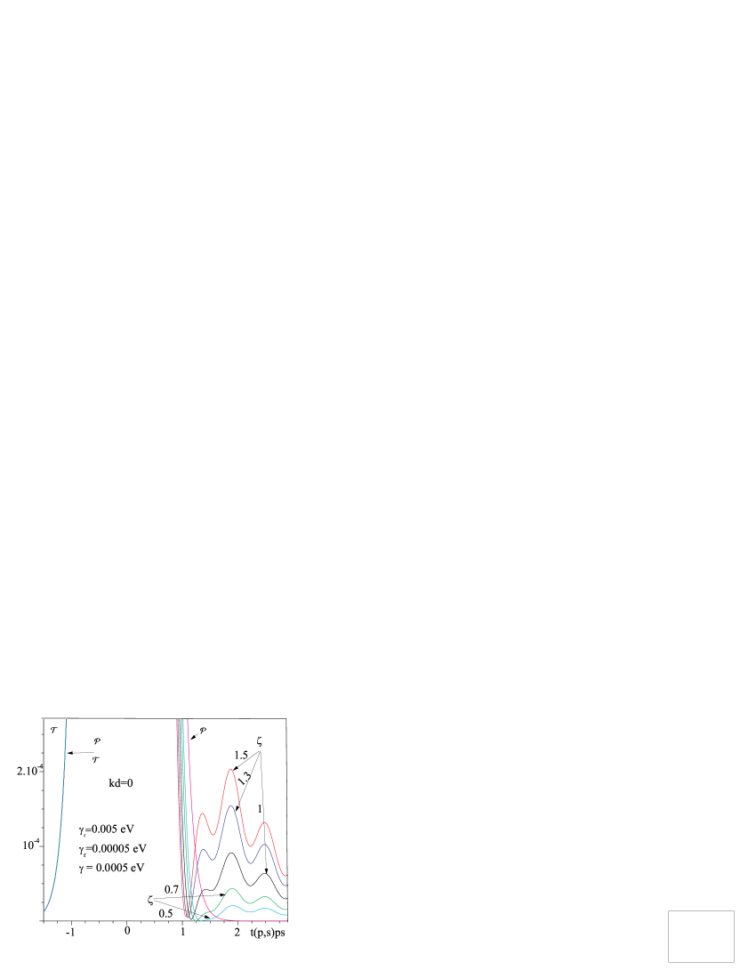
Рис. 7: The time dependance of the transmittance $\mathcal{T}$ in the case of narrow quantum wells $(kd=0)$, when the reflection from the QW borders is absent. $\Delta\omega=0.0065eV$.

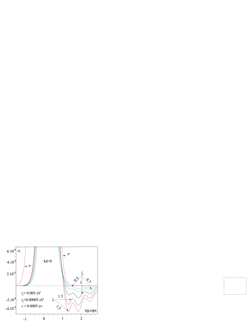
Рис. 8: The time dependance of the absorbance $\mathcal{A}$ in the case of narrow quantum wells $(kd=0)$, when the reflection from the QW borders is absent. $\Delta\omega=0.0065eV$.

Figs.6, 7, 8 demonstrate an influence of a heterogeneous medium on the transmittance $\mathcal{T}$ and on the energy part accumulated by the QW in the resonant transitions $\mathcal{A}$. In Fig.6 the parameters $\gamma_{\ell},\gamma$, $\gamma_{r}$ are the same as in Fig.3, and in Fig.7, 8 they are the same as in Fig.4, 5. In Fig.6 the curves $\mathcal{T}(p)$ are represented for $kd=1.5$, when a boundary reflection is largest one. At $kd=0$ and $kd=\pi$ that reflection disappears and an influence of $\zeta$ influences weakly on $\mathcal{T}(p)$. In Fig.7, 8 the curves $\mathcal{T}$ and $\mathcal{A}$ are calculated for $kd=0$. In such a case, the dependencies $\mathcal{T}(p)$ and $\mathcal{A}$ on $\zeta$ are stipulated only by the parameter $\zeta\gamma_{r}$. There appears a generation (a negative absorption) after pulse passing (Fig.8). The generation is stipulated by that that the electronic system does not absorb or radiate completely the energy, accumulated in resonant transitions during the time the pulse passes through the QW.

It is follows from the results represented above that taking into account the differences of the refraction indexes of the QW and barriers influences noticeably the reflectance. It is most strong when a reflection, stipulated by the resonant transitions in the QW, is a small value. The reflection from the QW boundaries depends on $kd$ and disappears at $kd=p\pi$, where $p$ is an integer. In these points the system QW - barriers looks like a homogeneous medium. A distinction from a homogeneous medium is only in a substitution of the radiative broadening $\epsilon^{\prime}\gamma_{r}$ by $\epsilon^{\prime}\zeta\gamma_{r}$.

The QW optical properties are like the optical properties of a plate with the parallel borders inserted into a medium with different refraction index. Indeed, if an absorption is small (for instance, if a carrying frequency is far away from the resonant frequencies of absorption ), then $\mathcal{R}$ and $\mathcal{T}$ are described by (V), which is just fair for such a plate under a pulse irradiation . A sharp decrease of reflection in the points $kd=p\pi$ takes place also nearby the resonant absorption frequencies.