Sharp Superconductor-Insulator Transition in Short Wires

Abstract

Recent experiments on short MoGe nanowires show a sharp superconductor-insulator transition tuned by the normal state resistance of the wire, with a critical resistance of $R_{c}\approx R_{Q}=h/(4e^{2})$. These results are at odds with a broad range of theoretical work on Josephson-like systems that predicts a smooth transition, tuned by the value of the resistance that shunts the junction. We develop a self-consistent renormalization group treatment of interacting phase-slips and their dual counterparts, correlated cooper pair tunneling, beyond the dilute approximation. This analysis leads to a very sharp transition with a critical resistance of $R_{Q}$. The addition of the quasi-particles’ resistance at finite temperature leads to a quantitative agreement with the experimental results. This self-consistent renormalization group method should also be applicable to other physical systems that can be mapped onto similar sine-Gordon models, in the previously inaccessible intermediate-coupling regime.

, , , and

1 Introduction

One of the most intriguing problems in low-dimensional superconductivity is the understanding of the mechanism that drives the superconductor-insulator transition (SIT). Experiments conducted on quasi-one-dimensional (1D) systems have shown that varying the resistivity and dimensions of thin metallic wires can suppress superconductivity [1, 2], and in certain cases lead to an insulating-like behavior [3, 4, 5, 6, 7].

Particularly interesting are recent experiments conducted on short MoGe nanowires [6] that explore the SIT tuned by the wire’s normal state resistance with a critical resistance $R_{c}\approx R_{Q}$. Resistance measurements of the quasi-1D MoGe nanowires reveal a strong temperature dependence that can be fitted with a modified LAMH theory [8, 9] of thermally activated phase-slips down to very low temperatures. However, for these narrow wires it appears that the LAMH theory is valid only in a narrow temperature window (see discussion in Sec. 2). Moreover, the LAMH analysis does not explain the appearance of a critical value of $R_{c}\approx R_{Q}$.

The universal critical resistance may suggest that, at a temperature much lower than the mean-field transition temperature, $T\ll T_{c}$, the wire acts as a superconducting (SC) weak link resembling a Josephson junction (JJ) connecting two SC leads. Schmid [10] and Chakravarty [11] showed that quantum phase-slip fluctuations in such a JJ lead to a SIT as a function of the junction’s shunt resistance, $R_{\mathrm{s}}$, with a critical resistance of $R_{Q}$, and that the resistance across the junction obeys the power law $R(T)\propto T^{2\left(\frac{R_{Q}}{R_{\mathrm{s}}}-1\right)}$. The theory was later extended to JJ arrays and SC wires [12, 13, 14]. Within these theories, a similar power-law prevails. However, contrary to this general prediction, Bollinger et al. [6] observe that the resistance of the MoGe wires exhibits a much stronger temperature dependence, even close to the SIT.

In a previous work [15], we have presented an approach that captures both the critical resistance of $R_{c}\approx R_{Q}$ at the SIT and the sharp decay of the resistance as a function of temperature. We treat the SIT in nanowires as a transition governed by quantum phase-slip (QPS) proliferation. This picture alone, however, cannot account for the observed strong temperature dependence of the resistance. We argued that the key ingredient left out in previous works is the inclusion of interactions between QPSs in such a finite-size wire, especially when the phase-slip population is dense.

We treat these interactions in a mean-field type approximation: when analyzing the behavior of a small segment of the wire, we include in its effective shunt-resistance the resistance due to phase-slips elsewhere in the wire. This scheme is motivated by numerical analysis of a related problem, an interacting pair of resistively-shunted JJs [16]. This self-consistent treatment primarily produces a sharp temperature dependence of the resistance. In addition, we include the effects of the Bogoliubov quasi-particles, which couple to the potential gradient created by each phase-slip [17]. Consequently, the resistance obtained in the experiment can be fitted without resorting to the LAMH theory beyond its limit of validity.

In this manuscript we generalize our previous results to the weak Josephson coupling limit, where conductance through the wire proceeds by Cooper pair tunneling. The use of a self-consistent treatment of correlated Cooper pair tunneling events leads to a similarly sharp SIT in the limit of highly resistive wires. This self-consistent approximation of phase-slip interactions should be applicable to similar multiple sine-Gordon models in the theoretically challenging intermediate-coupling regime.

The remainder of the manuscript is organized as follows. In Sec. 2 we discuss the validity of the LAMH theory for the wires in Ref. [6]. In Sec. 3 we summarize our previous results on the role of quantum phase-slip interactions in short wires, with details of derivation of the microscopic model in Appendix A. We generalize these results to highly resistive wires in Sec. 4, and present our conclusion in Sec. 5.

2 On the validity of the theory of thermally activated phase-slips in short wires

In an attempt to explain the strong temperature dependence of the resistance of quasi-1D MoGe nanowires, Bollinger et al. [6] have shown that the experimental curves can be fitted with a modified LAMH theory [8, 9] of thermally activated phase-slips, down to very low temperatures. Nevertheless, estimations based on the parameters of the wires in Ref. [6] (Table 1) suggest that most of the temperature range in the experiment lies outside of the region in which the theory is applicable. The theory of thermally activated phase-slips is based on the time-dependent Ginzburg-Landau description of a superconducting (SC) wire. This description is valid at temperatures higher than the gap, and far enough from $T_{c}$, such that fluctuation corrections are small, $T^{*}<T<T_{G}$. Here $T^{*}$ is defined by $\Delta(T^{*})=T^{*}$, with $\Delta(T)$ the temperature dependent order parameter, and $T_{G}=T_{c}(1-G\textit{i})$, with $G\textit{i}=\left[\frac{7\zeta(3)}{4\pi^{2}}\frac{R_{\xi}}{R_{Q}}\right]^{\frac{2}{3}}$ the Ginzburg-Levanyuk number for the quasi-1D wires, where $R_{\xi}=R_{\mathrm{W}}\xi/L$ is the normal resistance of a section of the wire of length $\xi$. For the wires in Ref. [6], the LAMH theory is valid only in a narrow temperature window as $T^{*}\approx 0.9T_{c}$, and estimates for $T_{G}$ range between $0.82T_{c}$ and $0.97T_{c}$ (see Fig. 1 and Table 1) [18, 19]. Moreover, the LAMH analysis does not explain the appearance of a critical resistance $R_{c}\approx R_{Q}$.

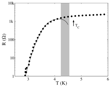
Figure 1: Validity of the LAMH theory for the data of wire No. 6 of Ref. [6] (see Table 1 for detailed parameters of the wire). The fitting parameters used to fit the data are the coherence length, $\xi=6.7$ nm, and the critical temperature, $T_{c}=4.7$ K, marked by an arrow. These fitting parameters yield a temperature range $T^{*}=4.23{\rm K}<T<T_{G}=4.55$ K, for which the LAMH theory is expected to be valid, shown in gray (see the text for a definition of $T^{*}$ and $T_{G}$).

This estimate suggests that most of the relevant temperature range in the experiment conducted in Ref. [6] is in the regime $T\ll\Delta(T)$, where quantum fluctuations become increasingly important. While the universal critical resistance supports the idea that the transition occurs due to quantum phase slip proliferation in a narrow constriction, the naive extension of the theory to SC wires [12, 13] cannot account for the observed sharp drop of the resistance. In the following section we will present a self-consistent treatment of quantum phase-slip proliferation, that captures both the critical resistance of $R_{c}\approx R_{Q}$ at the SIT and the sharp decay of the resistance as a function of temperature.

3 Low-resistance wires

The microscopic action for a SC wire can be obtained from the BCS Hamiltonian by a Hubbard–Stratonovich transformation followed by an expansion around the saddle point (see Appendix A)[20]. In the limit of low energy scales, $\omega,Dq^{2}~{}\ll~{}\Delta_{0}$, this yields [21]:

$$S = N_{0}A\Delta_{0}^{2}\int_{0}^{L}dx\int_{0}^{1/T}d\tau\left\{\frac{\rho^{2}}{2}\left[\ln\left(\rho^{2}\right)-1\right]\right.$$ (1)

$$\left.+2\xi_{0}^{2}\rho^{2}\left[\phi^{\prime 2}+\frac{\dot{\phi}^{2}}{v_{\phi}^{2}}\right]+\xi_{0}^{2}\left[\rho^{\prime 2}+\frac{\dot{\rho}^{2}}{v_{\rho}^{2}}\right]\right\},$$

where $L$ and $A$ are the wire’s length and cross section, respectively, $\xi_{0}^{2}=\pi D/8\Delta_{0}$, $v_{\rho}=\sqrt{(3\pi/2)D\Delta_{0}}$ the amplitude velocity, $v_{\phi}=\sqrt{\pi D\Delta_{0}(2AV_{c}N_{0}+1)}$ the phase velocity, $V_{c}$ the Fourier transform of the short-range Coulomb interaction, $N_{0}$ the density of states, $D$ the electronic diffusive constant in the normal state, and the SC order parameter is parameterized as $\Delta=\Delta_{0}\rho e^{i\phi}$, with $\Delta_{0}$ the mean-field solution. For the wires in Ref. [6], $2AV_{c}N_{0}\propto N_{\bot}\sim 1000\gg 1$, leading to $v_{\rho}\ll v_{\phi}\propto v_{\rho}\sqrt{N_{\bot}}$. Here $N_{\bot}=p_{F}^{2}A/\pi^{2}$ is the number of 1D channels in the wire.

This action supports QPS excitations, which are characterized by two distinct length scales: $v_{\rho}/\Delta_{0}\propto\xi\ll\xi\sqrt{N_{\bot}}\propto v_{\phi}/\Delta_{0}$. For very long wires, $\xi\ll\xi\sqrt{N_{\bot}}\ll L$, in the dilute phase-slip approximation, this problem can be mapped onto the perturbative limit of the $1+1$-dimensional sine-Gordon model [12]. In the opposite limit of very short wires, $L<\xi\ll\xi\sqrt{N_{\bot}}$, the system resembles a JJ and can be mapped onto the $0+1$-dimensional sine-Gordon model. However the wires in Ref. [6] appear to be in the intermediate regime, $\xi\ll L\ll\xi\sqrt{N_{\bot}}$. Hence, while phase-slips occur in different sections of the wire, they are indistinguishable, as each creates a phase fluctuation that spreads over distances larger than the wire itself.

Moreover, the wires in Ref. [6] have a sizable bare fugacity. Using Eq. (1), one can estimate the core action of a phase-slip of duration $\tau_{0}=1/\Delta_{0}$. Choosing the following trial function for a phase slip:

$$\phi = \arctan{\left(v_{\phi}\tau/x\right)}$$

$$\rho = \min{[\sqrt{\left(x/x_{0}\right)^{2}+\left(\Delta_{0}\tau\right)^{2}},1]},$$ (2)

and identifying the part of the action [Eq. (1)], that corresponds to $\rho\neq 1$ as the core action, we minimize this expression with respect to the phase-slip diameter, $x_{0}$. Keeping only leading terms in $N_{\bot}=\left(p_{F}^{2}A/\pi^{2}\right)$, this yields a core action of $S_{c}=\pi/8\sqrt{1/3(1-\epsilon)}R_{Q}/R_{\xi}$ [22]. Here $\epsilon=1-T/T_{c}$ is the reduced temperature and $R_{\xi}=R_{\mathrm{W}}\xi/L$ is the normal resistance of a section of length $\xi$. Using this expression, the measured values of $R_{\mathrm{W}}$ and $L$ (Table 1), and the assumption that $\xi\approx 20$ nm, the phase-slip fugacity is estimated to be $\zeta=e^{-S_{c}}\approx 0.05-0.45$ for the different wires. Consequently, in the critical region, $R_{\mathrm{W}}\approx R_{Q}$, there is a dense population of phase-slips that interact with one another; thus, the dilute phase-slip approximation is no longer a proper description.

The flow equation for the fugacity of a phase-slip anywhere in the wire is given by:

$$\frac{d\zeta}{dl} = \left(1-\frac{R_{Q}}{R_{\mathrm{s}}}\right)\zeta,$$ (3)

where $dl=-d\ln\Lambda$, and $\Lambda$ is the running RG scale. Eq. (3) treats the phase-slip as occurring on an effective JJ, with $R_{\mathrm{s}}$ being the effective shunting resistance of the entire wire. When $\zeta$ is small, $R_{\mathrm{s}}$ will include only the effective impedance of the leads. If $\zeta$ is not very small, we will need to include in Eq. (3) additional terms of higher powers of $\zeta$, which describe interactions between QPSs. To deal with a finite $\zeta$, we include the resistance due to other phase-slips in the wire in the effective shunt resistance of the junction, $R_{\mathrm{s}}$ [15]. This is akin to guessing the form of a complete resummation of higher-order $\zeta$ terms in Eq. (3) [23, 24].

This treatment was successfully tested by numerical analysis of a simpler analog of the system, an interacting pair of resistively shunted JJs [16]. In this work, Werner et. al studied the phase diagram and critical properties of the pair of JJs using Monte Carlo simulations and renormalization group calculations. The authors found that, in the region of the intermediate coupling fixed point, there is a remarkable resemblance in the critical behavior between the two-junction system and a single junction. In order to explain this resemblance, Werner et. al suggest that the two-junction system can be described by an approximate mean-field theory. In the mean-field approximation, each junction at criticality behaves as an independent junction and sees the other junction as an effective resistor whose resistance is determined by phase-slip events. This picture can account for the observed (and calculated) properties of the two junction-system at the superconducting to normal transition point.

The main physical intricacy of the self-consistent approach is the determination of the effective shunt resistance, $R_{\mathrm{s}}(\zeta)$, that governs the renormalization of the phase-slip fugacity [Eq. (3)]. A phase-slip produces time-varying phase gradients, and hence electrical fields. These dissipate through two channels in parallel: the SC channel - which has an effective resistance due to other phase slips, $R_{\mathrm{{ps}}}$ - and the quasi-particles conduction channel [17], which has resistance $R_{\mathrm{{qp}}}$. Once the disturbance reaches the leads, it also dissipates through the electro-dynamical modes of the large electrodes, whose real impedance is parameterized by $R_{\mathrm{{elec}}}$.

For $T\ll~{}T_{c}$, the resistance of the quasi-particles, $R_{\mathrm{{qp}}}$, can be approximated by

$$R_{\mathrm{{qp}}} = \frac{m}{e^{2}\tau_{\mathrm{n}}n_{\mathrm{{qp}}}}\frac{L}{A}=R_{\mathrm{n}}\frac{n}{n_{\mathrm{{qp}}}}\approx R_{\mathrm{n}}\sqrt{\frac{T}{2\pi\Delta_{0}}}e^{\frac{\Delta_{0}}{T}}.$$ (4)

Unfortunately, we lack a microscopic model for the impedance of the electrodes, as this depends on the details of the system such as the junction’s shape and material. However, we expect that at large scales, $T<\Lambda<\Delta$, the electrodes will act as a transmission line to the electromagnetic waves generated by the phase-slip. This transmission line is characterized by a real impedance which we denote as $R_{\mathrm{{elec}}}$, and use as a fitting parameter. Hence, the effective shunt resistance that affects the renormalization of the phase-slip fugacity at $T<\Lambda<\Delta$ [Eq. (3)] is

$$R_{\mathrm{s}}[\zeta(\Lambda)] = R_{\mathrm{{elec}}}+\left(\frac{1}{R_{\mathrm{{ps}}}[\zeta(\Lambda)]}+\frac{1}{R_{\mathrm{{qp}}}(T)}\right)^{-1}.$$ (5)

Fig. 2 shows the circuit we suggest describes the system.

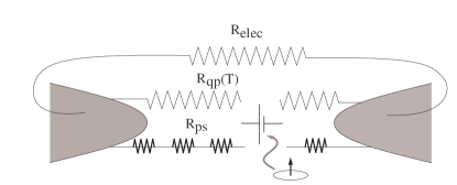
Figure 2: The effective electrical circuit for the nanowire. A phase-slip produces time-varying phase gradients, and hence electrical fields, that dissipate through the quasi-particle conduction channel, which has resistance $R_{\mathrm{{qp}}}$, and through the SC channel, that has an effective resistance due to other phase-slips, $R_{\mathrm{{ps}}}$. Once the disturbance reaches the edges, it also dissipates through the electro-dynamical modes of the large electrodes, whose real impedance is represented by $R_{\mathrm{{elec}}}$.

The resistance is measured in response to an applied DC current. In this zero frequency limit, the electrodes act as a capacitor connected in parallel to the wire. Therefore, the measured resistance is the total wire resistance, unaffected by the environment, which is cut off from the wire:

$$R_{\mathrm{{tot}}}(T) = \left(1/R_{\mathrm{{ps}}}[\zeta(T)]+1/R_{\mathrm{{qp}}}(T)\right)^{-1}.$$ (6)

The occurrence of a phase-slip causes a resistance in the otherwise SC wire through the relation $R_{\mathrm{{ps}}}\propto(L/\xi)\zeta^{2}$. Using this relation and Eq. (3), we can write an RG equation for the dimensionless resistance

$$\frac{d\zeta^{2}}{dl} = 2\zeta\frac{d\zeta}{dl}=2\left(1-\frac{R_{Q}}{R_{\mathrm{{s}}}(\zeta)}\right)\zeta^{2}$$

$$\Rightarrow\frac{d\left(R_{\mathrm{{ps}}}/R_{Q}\right)}{dl} = 2\left(1-\frac{R_{Q}}{R_{\mathrm{{s}}}(R_{\mathrm{{ps}}})}\right)\left(\frac{R_{\mathrm{{ps}}}}{R_{Q}}\right).$$ (7)

Integration of Eq. (3), with the effective resistance given in Eq. (5), from the ultraviolet (UV) cutoff $\Delta(T^{*})=T^{*}$ to the infrared cutoff $T$, yields $R_{\mathrm{{ps}}}(T)$.

The wire’s DC resistance Eq. (6), calculated using Eqs. (5) and (3), is plotted in Fig 3 (a) as a function of temperature for different $R^{*}$. Here $R^{*}\equiv R_{\mathrm{{tot}}}(T^{*})$ is the normal state resistance of the wire, at the UV cutoff $\Delta(T^{*})=T^{*}$. We assume that the wires are thin enough such that the mean-field transition from normal to SC is wide, and $R^{*}\approx R_{\mathrm{{tot}}}(T_{c}^{+})=R_{\mathrm{n}}$. For simplicity, we have assumed throughout our calculation that $\Delta(T)\approx\Delta_{0}$. This assumption holds in the low-temperature regime, $T\ll\Delta$, where the theory of QPSs, based on the effective action Eq. (1), is expected to be valid. The resistance of the environment is taken to be $R_{\mathrm{{elec}}}=0.1R_{Q}$. In practice, $\Delta$, $R^{*}$ and $R_{\mathrm{{elec}}}$ can be used as fitting parameters. Moreover, $R^{*}$ can be determined independently as the resistance measured below the drop that indicates passing through $T_{c}$ of the SC films (see Ref. [6]).

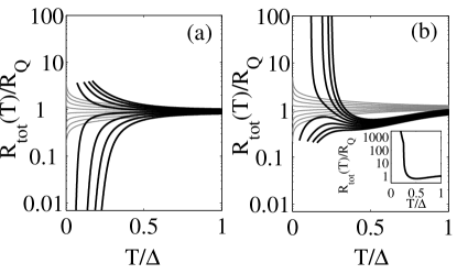
Figure 3: The total wire resistance, $R_{\mathrm{{tot}}}$, in units of $R_{Q}$ as a function of renormalized temperature $T/\Delta$ for different $R^{*}/R_{Q}$, ranging from $0.8$ (lower plot) to $1.01$ (upper plot) in increasing steps of $0.03$. The environment resistance was taken to be $R_{\mathrm{{elec}}}/R_{Q}=0.1$. Gray traces compare the total wire resistance $R_{\mathrm{{tot}}}(T)=\frac{R(T)R_{\mathrm{{qp}}}(T)}{R(T)+R_{\mathrm{{qp}}}(T)}$ to a single Josephson junction with $R(T)=R^{*}\left(T/\Delta\right)^{2(R_{Q}/R_{\mathrm{s}}-1)}$, and constant $R_{s}$. (a) The total wire resistance, $R_{\mathrm{{tot}}}(T)=\frac{R_{\mathrm{{ps}}}R_{\mathrm{{qp}}}(T)}{R_{\mathrm{{ps}}}+R_{\mathrm{{qp}}}(T)}$, in the limit of weak phase-slip fugacity calculated using Eqs. (5) and (3). The insulating plots are cutoff at temperature, $T_{0}$, for which $\zeta(T_{0})=1$ [see the discussion prior and subsequent to Eq. (8)]. (b) The total wire resistance, $R_{\mathrm{{tot}}}(T)=1/G_{\mathrm{{tot}}}(T)=\left(G_{\mathrm{{cp}}}(T)+1/R_{\mathrm{{qp}}}(T)\right)^{-1}$, in the weak Josephson coupling limit calculated using Eqs. (11) and (4). Here we have assumed the wire length is $L=5\xi$, where $\xi$ is the coherence length. The initial drop in the resistance of the high-resistance wires is a manifestation of the difference between the total wire resistance and the effective shunt resistance, in the presence of local quasi-particle relaxation, in the weak coupling limit. As the ratio between the wire length and the coherence length increases, the initial drop in the resistance becomes more pronounced. The low-resistance plots are cutoff at $T_{0}$, for which $J(T_{0})=1$. Inset: The resistance of the wire calculated in the self consistent approximation, Eq. (11), shows an initial sharp increase as the temperature is lowered, followed by a moderate increase. This moderation of the diverging resistance is due to the finite density of quasi-particles, present at finite temperature.

Eq. (3) is also applicable to a wire with $R^{*}>R_{Q}$. In this limit the fugacity increases in the renormalization process, and Eq. (3) is no longer valid for $\zeta\gtrsim 1$. For wires with $R^{*}>R_{Q}$, we overestimate the phase-slip fugacity as $\zeta(T^{*})=0.5$ and integrate Eq.(3), with

$$R_{\mathrm{s}}[\zeta(\Lambda)] = R_{\mathrm{{elec}}}+\left(\frac{1}{y_{\zeta}(R^{*})\zeta(\Lambda)^{2}}+\frac{1}{R_{\mathrm{{qp}}}(T)}\right)^{-1}\!\!\!\!\!\!\!\!,$$ (8)

from the UV cutoff, $\Delta(T^{*})=T^{*}$, down to the temperature $T_{0}$ for which $\zeta(T_{0})=1$. Here the proportionality constant $y_{\zeta}(R^{*})$ is set by the initial condition $R^{*}=\left(1/[y_{\zeta}(R^{*})\zeta(T^{*})^{2}]+1/R_{\mathrm{{qp}}}(T)\right)^{-1}$, with $\zeta(T^{*})=0.5$. The results are shown in Fig. 3 (a). Overestimating $\zeta(T^{*})$ gives an upper bound on $T_{0}$, where Eq. (3) is no longer applicable. Fig. 3 (a) shows that the transition between SC and insulating wires occurs for a critical resistance $R_{c}\approx R_{Q}$. However, in contrast to the standard Josephson junction theory (gray curves in Fig. 3 (a)), the transition is much sharper (notice the logarithmic scale).

	Measured Values			Fitting Values
Curve	$L(nm)$	$R_{\mathrm{W}}(k\Omega)$		$R^{*}(k\Omega)$		$\Delta(K)$		$R_{\mathrm{{elec}}}(k\Omega)$
$1$	177	005.	46	004.	2	02.	5	001.	2
$2$	43	3.	62	2.	62	2.	35	1.	25
$3$	63	2.	78	2.	13	3.	07	0.	66
$4$	93	3.	59	2.	89	3.	85	0.	55
$5$	187	4.	29	4.	5	6.	55	0.	31
$6$	99	2.	39	2.	09	4.	84	0.	4

Table 1: Summary of nanowire parameters, and the parameters used to fit the experimental data; $L$ is the length of the wire determined from SEM images, $R_{\mathrm{W}}$ is the wire’s normal state resistance, taken as the resistance measured below the film transition. Fitting parameters: $R^{*}=R_{\mathrm{tot}}(T=\Delta)$ is the wire’s resistance at the UV cutoff, $\Delta$ the SC order parameter, and $R_{\mathrm{{elec}}}$ the impedance of the electrodes at $T<\Lambda<\Delta$.

A comparison between the theoretical curves and the experimental data taken from Ref. [6] is shown in Fig.  4. The curves were calculated by fitting $R^{*}$, $\Delta$, and $R_{\mathrm{{elec}}}$. Since the theory of QPSs is expected to be valid at $T\ll\Delta$, deviations from the theoretical curves at high temperature are reasonable. In general, as $\Delta$ is proportional to $T_{c}$, increasing $\Delta$ shifts the sharp decay of the resistance to high temperatures. Both $R^{*}$ and $R_{\mathrm{{elec}}}$ affect the high temperature resistance, whereas $R^{*}$ and $\Delta$ control the width of the transition.

We have made an attempt to fit the data corresponding to the insulating wires of Ref. [6]. As the insulating wires are thinner, we expect a strong suppression of $T_{c}$ [2], which sets the scale for the high temperature cutoff $T\ll\Delta(T)$. Moreover, in these wires, the bare fugacity is estimated by $\zeta=e^{-S_{c}}\approx 0.32-0.84$, which results in a relatively high $T_{0}$, for which $\zeta(T_{0})=1$. Consequently, the theory of QPSs with $\zeta\lesssim 1$ is valid in a narrow range of temperatures. While we manage to fit the experimental curves in this regime of parameters, we do not present the results as our fits cover a range of $\sim 10$ data points, with three fitting parameters.

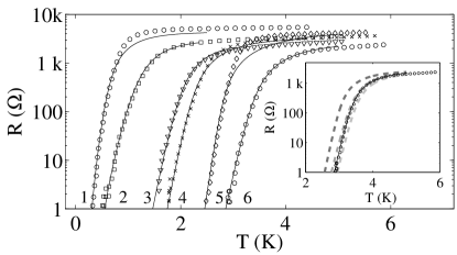
Figure 4: Comparison between the theory (solid line) and the experimental data [6]. Details of the wires, and fitting parameters are summarized in Table 1. Note that the estimated values for $R^{*}$ are in good agreement with the measured values of the resistance of the wire at $T=\Delta$. The discrepancies between theory and experiment occur for the longer wires (curves $1$ and $5$). In these wires the condition $v_{\phi}/\Delta_{0}\gg L$ might not hold, and one should consider additional renormalization at higher scales. Inset: The effect of an adjustment of the fit parameters, in roughly $10\%$ (from dark gray to light gray): $\Delta=4.356K$, $R_{\mathrm{{elec}}}=440\Omega$ and $R^{*}=1881\Omega$.

4 High-resistance wires

To better describe the insulating wires, we turn to the weak Josephson coupling limit where phase coherence across the wire is lost, and conductance proceeds by means of Cooper pair tunneling events across regions of fluctuating order parameter amplitude. The flow equation for the Josephson coupling anywhere in the wire is given by:

$$\frac{dJ}{dl} = \left(1-\frac{R_{\mathrm{s}}}{R_{Q}}\right)J.$$ (9)

Once more we expect that the Josephson tunneling between two such sections will be effected by all other tunneling events in the wire, via capacitive coupling.

The pair tunneling event leads to a finite conductance through the insulating wire, $G_{\mathrm{{cp}}}\propto J^{2}$. To use this relation and Eq. (9), we need to consider what the effective shunting resistance of an individual Josephson junction (a segment of length $\xi$) is. When a Cooper pair tunnels a distance $\xi$, a dipole of strength $2e\xi$ forms. It can relax either by locally fusing back through the quasi-particle channel, i.e, through a resistance $R_{\mathrm{{qp}}}(T)\xi/L$, or by the tunneling Cooper pair, and the hole it leaves behind increasing their separation, until they leave the system through the electrodes. The latter process implies the $2e$ charge goes through a resistance $R_{\mathrm{elec}}+\left(G_{\mathrm{{cp}}}[J(\Lambda)]+\frac{1}{R_{\mathrm{{qp}}}(T)}\right)^{-1}$. These two channels appear in parallel, see Fig. 5. Therefore the full shunting resistance is:

$$R_{\mathrm{s}}[J(\Lambda)]^{-1}=$$

$$\frac{1}{R_{\mathrm{elec}}+\left(\frac{R_{\mathrm{{qp}}}(T)}{R_{\mathrm{{qp}}}(T)G_{\mathrm{{cp}}}[J(\Lambda)]+1}\right)}+\frac{1}{R_{\mathrm{{qp}}}(T)\frac{\xi}{L}}.$$ (10)

Figure 5: The effective electrical circuit for the nanowire in the weak coupling limit. When a Cooper pair tunnels a distance $\xi$, a dipole of strength $2e\xi$ forms. It can relax either by locally fusing back through the quasi-particle channel, i.e, through a resistance $R_{\mathrm{{qp}}}(T)\xi/L$, or by increasing the separation between the tunneling Cooper pair and the hole it leaves behind, until they leave the system through the electrodes. The advancing Cooper pair can relax by means of successive tunneling events with resistance $1/G_{cp}$, or by exciting quasi-particles along the wire, with resistance $R_{qp}(T)$. Once more, as the excitation reaches the edges, it dissipates through the electro-dynamical modes of the large electrodes, whose real impedance is represented by $R_{\mathrm{{elec}}}$.

Thus the RG equation for the conductance, in units of $G_{Q}=4e^{2}/h$, is

$$\frac{d}{dl}\left(\frac{G_{\mathrm{{cp}}}}{G_{Q}}\right) = 2\left[1-\frac{R_{\mathrm{s}}(\Lambda)}{R_{Q}}\right]\left(\frac{G_{\mathrm{{cp}}}}{G_{Q}}\right),$$ (11)

where $R_{\mathrm{s}}$ is given by Eq. (4). The total resistance of the wire, $R_{\mathrm{{tot}}}(T)=1/G_{\mathrm{{tot}}}(T)=\left(G_{\mathrm{{cp}}}[J(T)]+1/R_{\mathrm{{qp}}}(T)\right)^{-1}$, calculated using Eqs. (4) and (11), is plotted in Fig 3 (b) as a function of temperature for different $R^{*}$. As mentioned above, $R^{*}\equiv R_{\mathrm{{tot}}}(T^{*})\approx R_{\mathrm{n}}$ is the normal state resistance of the wire, at the UV cutoff $\Delta(T^{*})=T^{*}$, which can be determined from resistance measurements at a temperature below the SC transition of the 2D films [6]. The order parameter is assumed to be constant throughout the calculation and the resistance of the environment is taken to be $R_{\mathrm{{elec}}}=0.1R_{Q}$. In Fig.  3 (b) we have assumed $L=5\xi$. In Ref. [6] the high-resistance wires are typically thinner, and are therefore expected to have a strong suppression of $T_{c}$ [2]. This will lead to a relatively large coherence length, and a smaller ratio $L/\xi$.

The initial drop in the resistance of the high-resistance wires is a manifestation of the difference between the total wire resistance and the effective shunt resistance, in the weak coupling limit. The local quasi-particle relaxation reduces the shunt resistance below $R_{Q}$ at $T\sim\Delta(T)$, causing an initial drop in the resistance. At lower temperature, the density of quasi-particles decreases exponentially, and $R_{\mathrm{qp}}\xi/L$ ceases to be smaller than $R_{Q}$. This leads to a decrease in the number of tunneling events causing the total resistance to increase. As the ratio between the length of the wire and the coherence length increases, the initial shunt resistance is smaller and the initial drop in the resistance becomes more pronounced.

The resistance of the wire, calculated in the self-consistent approximation, Eq. (11), shows an initial sharp increase as the temperature is lowered, followed by a moderate increase. As the pair tunneling drops rapidly to zero at a finite temperature, conductance persists due to the finite density of quasi particles. This residual conductance appears as a moderation of the diverging resistance, as shown in Fig 3 (b). Conversely, upon neglecting the interactions between different sections of the wire, the conductance due to independent Josephson tunneling shows a power law decay as a function of decreasing temperature, $G_{\mathrm{{cp}}}(T)=1/R^{*}\left(T/\Delta\right)^{-2(R_{Q}/R_{\mathrm{s}}-1)}$. Such a power law behavior leads to a finite conductance at finite temperature, which shunts the highly resistive contribution of the quasi-particles.

Eq. (11) is also applicable to a wire with $R^{*}<R_{Q}$. In this limit the pair tunneling increases in the renormalization process, and Eq. (11) is no longer valid for $J\gtrsim 1$. We estimate bare Josephson coupling as $J(T^{*})=0.5$ and integrate Eq. (9) with

$$R_{\mathrm{s}}(\Lambda) = R_{\mathrm{elec}}+\left(y_{J}(R^{*})J(\Lambda)^{2}+\frac{1}{R_{\mathrm{{qp}}}(T)}\right)^{-1},$$ (12)

from the UV cutoff, $\Delta(T^{*})=T^{*}$, down to the temperature $T_{0}$ for which $J(T_{0})=1$. Once more, the proportionality constant is set by the initial condition $R^{*}=\left[y_{J}(R^{*})J(T^{*})^{2}+1/R_{\mathrm{{qp}}}(T)\right]^{-1}$. The results are shown in Fig. 3 (b).

When we use the resistive wire theory, we must consider the following caveat: If the Josephson coupling between segments of the wire is only perturbative, then the phase of the order parameter fluctuates locally as a function of time. If the frequency scale of this fluctuation is comparable to the order-parameter magnitude, then there should also be low lying sub-gap density of states in the wire, that we don’t take into account. The theory in this section assumes that the phase fluctuations are sufficiently slow such that the sub-gap states can be ignored.

5 Conclusion

In conclusion, we studied the effect of interactions between QPSs in short SC wires, beyond the dilute phase-slip approximation. Our analysis shows that treating these interactions in a self-consistent manner produces a sharp superconductor-insulator transition with a critical resistance $R_{c}\approx R_{Q}$, in agreement with recent experiments [6]. Moreover, we have shown that adding the resistance of the BdG quasi-particles leads to a quantitative agreement with the experimental curves. In the dual weak Josephson coupling limit, this self-consistent RG treatment produces a similar sharp insulator-superconductor transition. The sharp drop in the conductance of the insulating wires in this limit is shown to be accompanied by a residual conductance due to the density of quasi-particles at this finite temperature. Our method should be applicable to a wider range of physical problems which involve the proliferation of topological defects with a sizable bare fugacity. In particular, it could be applied to the study of a Luttinger liquid with an extended impurity [25].

We thank E. Demler, and P. Werner. Special thanks to A. Bezryadin for making his data available to us. This study was supported by a DIP grant and by an ISF grant.

Appendix A Derivation of microscopic action

Consider a system of electrons in the diffusive limit that interact via Coulomb repulsion and the phonon mediated BCS interaction. This is described by the Hamiltonian $H=H_{0}+H_{int}+H_{BCS}$:

$$H_{0} = \sum_{\sigma}\int d^{3}r\psi_{\sigma}^{\dagger}(r)\left(-\frac{\nabla_{r}^{2}}{2m}+\sum_{i}u(r-r_{i})\right)\psi_{\sigma}^{\dagger}(r)$$

$$H_{int} = \sum_{\sigma,\sigma^{\prime}}\int d^{3}rd^{3}r^{\prime}\psi_{\sigma}^{\dagger}(r)\psi_{\sigma}(r)\frac{e^{2}}{|r-r^{\prime}|}\psi_{\sigma^{\prime}}^{\dagger}(r^{\prime})\psi_{\sigma^{\prime}}(r^{\prime})$$

$$H_{BCS} = -\lambda\sum_{\sigma}\int d^{3}r\psi_{\sigma}^{\dagger}(r)\psi_{\sigma}(r)\psi_{\bar{\sigma}}^{\dagger}(r)\psi_{\bar{\sigma}}(r),$$ (13)

where $\psi_{\sigma}^{\dagger}(r)$ and $\psi_{\sigma}(r)$ are electron creation and annihilation operators, the Fourier transform of the Coulomb interaction in 1D $V_{c}(q)\sim\log{q}$ is taken to be constant, and $u(r-r_{i})$ is the impurity potential at point $r$ due to an impurity at point $r_{i}$. We assume that the impurity potential is $\delta$ correlated, $\langle u(r)\rangle=0$, and $\langle u(r)u(r^{\prime})\rangle=\frac{1}{2\pi N_{0}\tau}\delta(r-r^{\prime})$, where $\tau$ is the impurity scattering time, and $N_{0}$ is the 3D density of states. Following Ref. [26], we apply a Hubbard–Stratonovich transformation in order to rewrite the BCS interaction and the Coulomb interaction. The partition function becomes

$$Z = \int D\Delta D\Delta^{*}D\rho D\psi D\psi^{\dagger}e^{-S},$$

where

$$S = S_{0}+\int dx\frac{|\Delta(x)|^{2}}{\lambda}$$ (14)

$$+ \int dx\left\{\Delta(x)^{*}\psi_{\downarrow}(x)\psi_{\uparrow}(x)+\Delta(x)\psi_{\uparrow}^{\dagger}(x)\psi_{\downarrow}^{\dagger}(x)\right\}$$

$$+ \frac{1}{2}\int dxdx^{\prime}\rho(x)V_{c}^{-1}(x-x^{\prime})\rho(x^{\prime})$$

$$+ i\int dx\rho(x)\left\{\psi_{\uparrow}^{\dagger}(x)\psi_{\uparrow}(x)+\psi_{\downarrow}^{\dagger}(x)\psi_{\downarrow}(x)\right\},$$

and $x\equiv(\textbf{r},\tau)$. Integrating over the fermionic fields, the effective action in Nambu-Gorkov spinor notation reads

$$S = \int dx\lambda^{-1}|\Delta(x)|^{2}-Tr\ln{G}^{-1}$$ (15)

$$+\frac{1}{2}\int dxdx^{\prime}\rho(x)V_{c}^{-1}(x-x^{\prime})\rho(x^{\prime})$$

with

$$G^{-1} = \left(\begin{array}[]{cc}\partial_{\tau}-\xi+i\rho&\Delta\\ \Delta^{*}&\partial_{\tau}+\xi-i\rho\\ \end{array}\right),$$ (18)

and $\xi=-\nabla^{2}/2m-\mu$. One can treat the presence of nonmagnetic impurities by including a self-energy diagram that describes the dressing of the electron line by impurities. As a result, the frequencies and the order parameter are replaced by $\tilde{\omega}=\eta\omega$ and $\tilde{\Delta}=\eta\Delta$, with $\eta=\left(1+1/(2\tau\sqrt{\omega^{2}+\Delta_{0}^{2}})\right)$ [27]. Moreover, when calculating polarization bubbles (see section A.2), one must sum over the impurity ladder (namely impurity lines connecting the two Green’s functions in the polarization bubble).

A.1 Uniform order parameter

In the case of a uniform order parameter, the action in Eq. (15) can be greatly simplified. In this limit, the order parameter $\Delta$ can be chosen to be real and the action reduces to [28]

$$S[\Delta] = \int dx\lambda^{-1}|\Delta(x)|^{2}$$ (19)

$$-T\sum_{\omega}\nolimits^{\prime}\int\frac{d^{3}p}{(2\pi)^{3}}\ln{\left(\tilde{\omega}^{2}+\xi_{p}^{2}+\tilde{\Delta}^{2}\right)}.$$

A variation of the action in Eq. (15) with respect to $\Delta^{*}$ yields the BCS gap-equation

$$\frac{\Delta_{0}}{\lambda} = \pi N_{0}T\sum_{\omega}\nolimits^{\prime}\frac{\Delta_{0}}{\sqrt{\omega^{2}+\Delta_{0}^{2}}},$$ (20)

where the sum $\sum_{\omega}\nolimits^{\prime}$ indicates that the frequencies are cut off at the Debye frequency, $\omega_{D}$. In order to evaluate the sum in Eq. (19), we replace $S[\Delta]$ by

$$S[\Delta]-S[0] = \int_{0}^{\Delta}\frac{\partial S[\Delta]}{\partial\Delta},$$ (21)

where

$$\frac{\partial S[\Delta]}{\partial\Delta} = \frac{2\Delta}{\lambda}-2\tilde{\Delta}T\sum_{\omega}\nolimits^{\prime}\int d^{3}p\frac{1}{\left(\tilde{\omega}^{2}+\xi_{p}^{2}+\tilde{\Delta}^{2}\right)}$$ (22)

$$= \frac{2\Delta}{\lambda}-2\pi N_{0}T\sum_{\omega}\nolimits^{\prime}\frac{\Delta}{\sqrt{\omega^{2}+\Delta^{2}}}.$$

We have substracted $S[0]$ to avoid divergences. As $S[0]$ is independent of $\Delta$, this choice does not affect our final results. Integrating with respect to $\Delta$ results in the following action

$$S[\Delta]-S[0] = \frac{\Delta^{2}}{\lambda}-4\pi N_{0}T\sum_{\omega=0}^{\omega_{D}}\left(\sqrt{\omega^{2}+\Delta^{2}}-\omega\right)$$ (23)

$$\approx \frac{\Delta^{2}}{\lambda}-N_{0}\Delta^{2}\left[\frac{1}{2}+\ln{\left(\frac{2\omega_{D}}{\Delta}\right)}\right],$$

which can be written as

$$S[\Delta]-S[0] = \frac{N_{0}\Delta^{2}}{2}\left[\ln\left({\frac{\Delta^{2}}{\Delta_{0}^{2}}}\right)-1\right].$$ (24)

A.2 Fluctuations around the mean-field solution

The action describing phase and amplitude fluctuations is obtained by expanding Eq. (15) around the mean-field saddle point solution $\Delta=\Delta_{0}$. Dividing the fluctuations into real and imaginary parts, $\delta\Delta=\Delta_{L}+i\Delta_{T}$, which are connected to amplitude and phase variations, the fluctuations around the mean field are given by

$$S = \int dx\frac{|\Delta_{0}|^{2}}{\lambda}+\frac{\Delta_{L}^{2}+\Delta_{T}^{2}}{\lambda}$$ (25)

$$+\frac{1}{2}\int dxdx^{\prime}\rho(x)V_{c}^{-1}(x-x^{\prime})\rho(x^{\prime})-Tr\ln{G}_{0}^{-1}$$

$$-Tr\sum_{n=2}^{\infty}\frac{(-1)^{n+1}}{n}\left({G}_{0}\delta{G}^{-1}\right)^{n}.$$

Here

$${G}_{0} = \frac{1}{\tilde{\omega}^{2}+\xi^{2}+\tilde{\Delta}_{0}^{2}}\left(\begin{array}[]{cc}-i\tilde{\omega}-\xi&\tilde{\Delta}_{0}\\ \tilde{\Delta}_{0}^{*}&-i\tilde{\omega}+\xi\\ \end{array}\right)$$ (28)

$$\delta{G}^{-1} = \left(\begin{array}[]{cc}i\rho&\Delta_{L}+i\Delta_{T}\\ \Delta_{L}-i\Delta_{T}&-i\rho\\ \end{array}\right).$$ (31)

Keeping only leading terms in $\rho$, $\Delta_{L}$ and $\Delta_{T}$, we find that the partition function can be written as

$$Z = \int D\Delta_{L}D\Delta_{T}\ D\rho e^{-S_{eff}\left[\Delta_{L},\Delta_{T},\rho\right]},$$ (32)

with the effective action

$$S_{\mathrm{eff}} = -\int{\,\mathchar 22\relax\mkern-9.0mu{\!d}}q\left(\begin{array}[]{ccc}\Delta_{L}&\Delta_{T}&\rho\\ \end{array}\right)_{q}V^{-1}(q)\left(\!\!\begin{array}[]{c}\Delta_{L}\\ \Delta_{T}\\ \rho\\ \end{array}\!\!\right)_{-q}\!\!\!\!\!\!,$$ (37)

where we have introduced a shorthand notation $\int{\,\mathchar 22\relax\mkern-9.0mu{\!d}}q=AT\sum_{\omega_{n}}\int dq/2\pi$ and $A$ is the wire’s cross section. The screened potentials are given by [29]

$$V^{-1}(q)=$$

$$\left(\!\!\!\begin{array}[]{ccc}-\frac{1}{\lambda}+\Pi_{\Delta_{L}\Delta_{L}}\!\!&0\!\!&0\\ 0\!\!&-\frac{1}{\lambda}+\Pi_{\Delta_{T}\Delta_{T}}\!\!&\Pi_{\Delta_{T}\rho}\\ 0\!\!&-\Pi_{\Delta_{T}\rho}\!\!&\frac{1}{2AV_{c}}+\Pi_{\rho\rho}\\ \end{array}\!\!\!\right).$$ (41)

In the above, $\Pi_{\alpha\beta}$ is the polarization bubble obtained by integrating out the electronic degrees of freedom, with the vertices $\alpha$ and $\beta$ corresponding to the incoming and outgoing bosonic fields.

In the dirty limit $ql,\Omega\tau\ll 1$, where $q$ and $\Omega$ are the transferred momentum and frequency, respectively, and $l$ and $\tau$ are the mean free path and impurity scattering time, we find

$$\Pi_{\Delta_{L}\Delta_{L}}(q,\Omega) = \pi N_{0}T\sum_{\omega}\left\{\left[1+\frac{\omega\omega^{\prime}-\Delta_{0}^{2}}{WW^{\prime}}\right]\right.$$

$$\times \left.\frac{1}{W+W^{\prime}+Dq^{2}}\right\}$$

$$\Pi_{\Delta_{T}\Delta_{T}}(q,\Omega) = \pi N_{0}T\sum_{\omega}\left\{\left[1+\frac{\omega\omega^{\prime}+\Delta_{0}^{2}}{WW^{\prime}}\right]\right.$$

$$\times \left.\frac{1}{W+W^{\prime}+Dq^{2}}\right\}$$

$$\Pi_{\rho\rho}(q,\Omega) = N_{0}-\pi N_{0}T\sum_{\omega}\left\{\left[1-\frac{\omega\omega^{\prime}+\Delta_{0}^{2}}{WW^{\prime}}\right]\right.$$

$$\times \left.\frac{1}{W+W^{\prime}+Dq^{2}}\right\}$$

$$\Pi_{\Delta_{T}\rho}(q,\Omega) = -\pi N_{0}T\sum_{\omega}\frac{\Delta_{0}\Omega}{WW^{\prime}}\frac{1}{W+W^{\prime}+Dq^{2}}$$ (42)

$$= -\Pi_{\rho\Delta_{T}}(q,\Omega).$$

Here $\omega^{\prime}=\omega+\Omega$, $W=\sqrt{\omega^{2}+\Delta_{0}^{2}}$, $W^{\prime}=\sqrt{\omega^{\prime 2}+\Delta_{0}^{2}}$ and $D=\tau v_{F}^{2}/3$ is the diffusion constant. In the low temperature limit, for $q\ll\xi\sim\xi_{0}$ and $\Omega\ll\Delta_{0}$, where $\xi_{0}$ is the zero temperature coherence length, these may be approximated by

$$\Pi_{\Delta_{L}\Delta_{L}}(q,\Omega)-\lambda^{-1}\approx-N_{0}\left(1+\frac{\Omega^{2}}{12\Delta_{0}^{2}}+\frac{\pi}{8}\frac{Dq^{2}}{\Delta_{0}}\right)$$ (43)

$$\Pi_{\Delta_{T}\Delta_{T}}(q,\Omega)-\lambda^{-1}\approx-N_{0}\left(\frac{\Omega^{2}}{4\Delta_{0}^{2}}+\frac{\pi}{4}\frac{Dq^{2}}{\Delta_{0}}\right)$$

$$\Pi_{\rho\rho}(q,\Omega)\approx N_{0}\left(1-\frac{1}{6}\frac{\Omega^{2}}{\Delta_{0}^{2}}\right)$$

$$\Pi_{\Delta_{T}\rho}(q,\Omega)\approx-\frac{N_{0}\Omega}{2\Delta_{0}}\left(1-\frac{1}{6}\frac{\Omega^{2}}{\Delta_{0}^{2}}-\frac{\pi}{8}\frac{Dq^{2}}{\Delta_{0}}\right)\!\!.$$

Note that close to $T_{c}$, namely in the limit $\Delta\ll\Omega,Dq^{2}\ll T$, the polarization bubble $\Pi_{\Delta_{L}\Delta_{L}}=\Pi_{\Delta_{T}\Delta_{T}}\approx-N_{0}\left(\frac{\pi}{8}\frac{|\Omega|+Dq^{2}}{T}-\ln\left(\frac{1.13\omega_{D}}{T}\right)\right)$, which reproduces the time-dependent Ginzburg-Landau (TDGL). The term $\sim|\Omega|$ describes dissipation. Its emergence is a result of the fact that the polarization bubbles describe the response of the electronic system, in equilibrium. Hence, we have assumed the existence of a relaxation mechanism that allows the electrons to return to equilibrium. This assumption should be taken with caution when studying transport close to the phase transition, as typical time scales close to the phase transition diverge.

We perform the Gaussian integration over the field $\rho$ to obtain an effective action for $\Delta_{T}$. This leads to an extra term in the $\Delta_{T}$ propagator, so that

$$-\frac{1}{\lambda} + \Pi_{\Delta_{T}\Delta_{T}}\rightarrow$$ (44)

$$-\frac{1}{\lambda}+\Pi_{\Delta_{T}\Delta_{T}}+\frac{\left(\Pi_{\Delta_{T}\rho}\right)^{2}}{\left(2V_{c}\right)^{-1}+\Pi_{\rho\rho}}$$

$$\approx -N_{0}\left(\frac{\pi}{4}\frac{Dq^{2}}{\Delta_{0}}+\frac{\Omega^{2}}{4\Delta_{0}^{2}}\frac{1}{2AV_{c}N_{0}+1}\right).$$

Finally, the effective action describing real and imaginary parts of the fluctuation in the order parameter is

$$S_{\mathrm{fluc}} = N_{0}\int{\,\mathchar 22\relax\mkern-9.0mu{\!d}}q\left\{\left(1+\frac{\Omega^{2}}{12\Delta_{0}^{2}}+\frac{\pi}{8}\frac{Dq^{2}}{\Delta_{0}}\right)|\Delta_{L}(q)|^{2}\right.$$ (45)

$$\!\!\!\!\!\!\!\!\!\left.\left(\frac{\pi Dq^{2}}{4\Delta_{0}}+\frac{\Omega^{2}}{4\Delta_{0}^{2}}\frac{1}{2AV_{c}N_{0}+1}\right)|\Delta_{T}(q)|^{2}\!\!\right\}\!\!.$$

We note that the general expression for the uniform fluctuations of the magnitude of the order parameter, Eq. (24), reduces to the form given by $\Pi_{\Delta_{L}\Delta_{L}}$ in Eq. (45), under the substitution $\Delta=\Delta_{0}+\Delta_{L}$. One can show [30] that the real and imaginary parts of the order parameter, $\Delta_{L}/\Delta_{0}$ and $\Delta_{T}/\Delta_{0}$, are related under gauge transformation to the amplitude, $\rho$ and phase, $\phi$ of the order parameter, respectively. Collecting all terms and writing the action in terms of the amplitude and phase, we have

$$S = N_{0}A\Delta_{0}^{2}\int_{0}^{L}dx\int_{0}^{1/T}d\tau\left\{\frac{\rho^{2}}{2}\left[\ln\left(\rho^{2}\right)-1\right]\right.$$ (46)

$$\left.+2\xi_{0}^{2}\rho^{2}\left[\phi^{\prime 2}+\frac{\dot{\phi}^{2}}{v_{\phi}^{2}}\right]+\xi_{0}^{2}\left[\rho^{\prime 2}+\frac{\dot{\rho}^{2}}{v_{\rho}^{2}}\right]\right\},$$

with $v_{\phi}$ and $v_{\rho}$ as given in Sec. 3.

References

- [1] P. Xiong, A. V. Herzog, and R. C. Dynes, Phys. Rev. Lett. 78, 927 (1997).
- [2] Y. Oreg and A. M. Finkel’stein, Phys. Rev. Lett. 83, 191 (1999).
- [3] F. Sharifi, A. V. Herzog, and R. C. Dynes, Phys. Rev. Lett. 71, 428 (1993).
- [4] A. Bezryadin, C. N. Lau, and M. Tinkham, Nature 404, 971 (2000).
- [5] C. N. Lau, N. Markovic, M. Bockrath, A. Bezryadin, and M. Tinkham, Phys. Rev. Lett. 87, 217003 (2001).
- [6] A. T. Bollinger, A. Rogachev, and A. Bezryadin, Europhys. Lett. 76, 505 (2006).
- [7] A. T. Bollinger, R. C. Dinsmore III, A. Rogachev, and A. Bezryadin, cond-mat/0707.4532
- [8] J. S. Langer and V. Ambegaokar, Phys. Rev. 164, 498 (1967).
- [9] D. E. McCumber and B. I. Halperin, Phys. Rev. B 1, 1054 (1970).
- [10] A. Schmid, Phys. Rev. Lett. 51, 1506 (1983).
- [11] S. Chakravarty, Phys. Rev. Lett. 49, 681 (1982).
- [12] H. P. Büchler, V. B. Geshkenbein, and G. Blatter, Phys. Rev. Lett. 92, 067007 (2004).
- [13] G. Refael, E. Demler, Y. Oreg, and D. S. Fisher, Phys. Rev. B 75, 014522 (2007).
- [14] G. Refael, E. Demler, and Y. Oreg, In preparation.
- [15] D. Meidan, Y. Oreg, and G. Refael, Phys. Rev. Lett. 98, 187001 (2007).
- [16] P. Werner, G. Refael, and M. Troyer, J. Stat. Mech. P12003 (2005).
- [17] This could be seen by considering a time dependent Bogoliubov de Gennes (BdG) equation, with a time dependent phase: . By the canonical transformation , we produce an effective potential for the quasi-particles in the BdG Hamiltonian.
- [18] This is in contrasted to the well established fit of the LAMH theory to tin whisker crystals [19], where the theory is applicable for , and the range of fitting was . Here is the reduced temperature.
- [19] R. S. Newbower, M. R. Beasley, and M. Tinkham, Phys. Rev. B 5, 864 (1972).
- [20] The expansion is done in the dirty limit, , where is the scattering mean free time.
- [21] D. S. Golubev and A. D. Zaikin, Phys. Rev. B 64, 014504 (2001).
- [22] Robert A. Smith and Yuval Oreg (unpublished).
- [23] For instance, adding the next order term, , [24] to Eq. (3), can be thought of as modifying by . .
- [24] S. A. Bulgadaev, Phys. Lett. A 86, 213 (1981).
- [25] C. L. Kane and M. P. A. Fisher, Phys. Rev. B 46, 15233 (1992).
- [26] U. Eckern and F. Pelzer, J. Low. Temp. Phys. 73, 433 (1988).
- [27] N. Kopnin, Theory of nonequilibrium superconductivity (Clarendon Press, Oxford, 2001).
- [28] U. Eckern, G. Schön, and V. Ambegaokar, Phys. Rev. B 30, 6419 (1984).
- [29] R. A. Smith, M. Y. Reizer, and J. W. Wilkins, Phys. Rev. B 51, 6470 (1995).
- [30] A. van Otterlo, D. S. Golubev, A. D. Zaikin, and G. Blatter, Eur. Phys. J. B 10, 131 (1999).