Clumpy photon-dominated regions in Carina

Abstract

Context. The Carina region is an excellent astrophysical laboratory for studying the feedback mechanisms of newly born, very massive stars within their natal giant molecular clouds (GMCs) at only 2.35 kpc distance.

Aims. We use a clumpy PDR model to analyse the observed intensities of atomic carbon and CO and to derive the excitation conditions of the gas.

Methods. The NANTEN2-4m submillimeter telescope was used to map the [C i] ${}^{3}P_{1}-^{3}P_{0}$, ${}^{3}P_{2}-^{3}P_{1}$ and CO 4–3, 7–6 lines in two $4^{\prime}\times 4^{\prime}$ regions of Carina where molecular material interfaces with radiation from the massive star clusters. One region is the northern molecular cloud near the compact OB cluster Tr 14, and the second region is in the molecular cloud south of $\eta$Car and Tr 16. These data were combined with ¹³CO SEST spectra, HIRES/IRAS $60\,\mu$m and $100\,\mu$m maps of the FIR continuum, and maps of 8$\,\mu$m IRAC/Spitzer and MSX emission.

Results. We used the HIRES far-infrared dust data to create a map of the FUV field heating the gas. The northern region shows an FUV field of a few $10^{3}$ in Draine units while the field of the southern region is about a factor 10 weaker. While the IRAC 8$\,\mu$m emission lights up at the edges of the molecular clouds, CO and also [C i] appear to trace the H₂ gas column density. The northern region shows a complex velocity and spatial structure, while the southern region shows an edge-on PDR with a single Gaussian velocity component. We constructed models consisting of an ensemble of small spherically symmetric PDR clumps within the $38^{\prime\prime}$ beam (0.43 pc), which follow canonical power-law mass and mass-size distributions. We find that an average local clump density of $2\,10^{5}$ cm^-3 is needed to reproduce the observed line emission at two selected interface positions.

Conclusions. Stationary, clumpy PDR models reproduce the observed cooling lines of atomic carbon and CO at two positions in the Carina Nebula.

1 Introduction

1.1 The importance of atomic carbon

The fine structure lines of atomic carbon are strong coolants of the interstellar medium (ISM) throughout the universe: in Galactic clouds (e.g. Jakob et al. 2007), in the Milky Way as a whole (Fixsen et al. 1999), as well as in external galaxies (Bayet et al. 2006; Kramer et al. 2005) up to high redshifts (Weiss et al. 2003). Large-scale observations of Galactic clouds show [C i] emission coincident with that of CO. This holds for giant molecular clouds (GMCs) (Sakai et al. 2006), as well as for rather quiescent dark clouds (Tatematsu et al. 1999). It has therefore been suggested that [C i] is a more reliable tracer of the molecular cloud masses in external galaxies than CO (Papadopoulos et al. 2004). However, all steady-state models of photon-dominated regions (PDRs) predict that atomic carbon is formed in a surface layer by recombination of C⁺ and dissociation of CO. This appears to be in contradiction with atomic carbon emission which is observed even at large distances from UV sources. The dynamics of the ISM may play a decisive role, allowing to explain the distribution of [C i] with time dependent chemical models (Oka et al. 2004; Störzer et al. 1997).

However, stationary, but clumpy PDR models have been successful in explaining e.g. extended [C i] ${}^{3}P_{1}-^{3}P_{0}$ and ¹³CO $2-1$ emission in S 140 (Spaans 1996; Spaans & van Dishoeck 1997). Inside a clumpy PDR, the UV radiation can penetrate much deeper than it would be possible in a homogeneous layer (Boissé 1990). Meixner & Tielens (1993) showed that the line intensities of all lines are enhanced compared to a homogeneous model with the same average density. Juvela et al. (2001) presented a model to apply Monte Carlo radiative transfer calculations to the results of magnetohydrodynamic calculations to account for a clumpy and turbulent structure. They also found that local density condensations lead to an increased cooling efficiency and reduced photon trapping. Another approach is to describe both the turbulent velocity field and the density structure by their statistical properties. Hegmann et al. (2007) calculate CO cooling rates based on a stochastic radiative transfer model, which accounts for density and velocity fluctuations with a finite correlation length.

Here, we study the distribution of atomic carbon and warm CO in the Carina star forming region and test clumpy models using the KOSMA-$\tau$ PDR model (Störzer et al. 1996; Röllig et al. 2007) to derive the excitation conditions of the gas. Spaans et al. model the inhomogeneous structure with a Monte-Carlo code, assuming a fixed clump/interclump density ratio of 10. In contrast, we assume that all emission analyzed stems from the clumps. The influence of the interclump medium or a halo leading to pre-shielding of CO has been discussed by Bensch (2006) and Bensch et al. (2003), who also used KOSMA-$\tau$, but is not considered here. To describe the clumpy structure, we assume that the clumps are distributed following the canonical clump mass and mass-size distributions which have been found in molecular clouds.

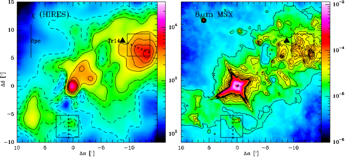
Figure 1: Overview of the Carina clouds near $\eta$Car lying at 0/0 10:45:03.59 -59:41:04.3 (J2000) at the center of the Tr 16 cluster. Left: Estimate of the FUV flux $\chi$ in Draine units at a resolution of $\sim 1^{\prime}$ and derived from HIRES/IRAS. Dashed contours range from 400 to 800 in steps of 200. Solid contours range from $10^{3}$ to $5\,10^{3}$ in steps of $10^{3}$. Right: MSX emission at 8 $\mu$m at a resolution of $\sim 20^{\prime\prime}$. Contours are 1 to 10 in steps of $1\leavevmode\nobreak\ 10^{-5}$ Wm^-2sr^-1 (cf. Figs. 7, 11 in Rathborne et al. 2002). Note the diffraction artefacts near $\eta$Car. The center position of the OB cluster Tr 14 is marked by a triangle. The two $4^{\prime}\times 4^{\prime}$ regions mapped with NANTEN2 are delineated by boxes. Crosses in the left panel mark two cuts discussed in the text.

Table 1: Physical parameters derived from the observed integrated intensities $I$ in K kms^-1 and intensity ratios $R^{74}_{\rm CO}$=$I$(CO 7–6)/$I$(CO 4–3), $R^{21}_{\rm C}$=$I$([C i]2–1)/$I$([C i]1–0), $R^{14}_{\rm CCO}$=$I$([C i]1–0)/$I$(CO 4–3) from Gaussian fits to the line profiles at two interface positions. The calibration error of the integrated intensities is estimated to be 15%.

$\Delta\alpha/\Delta\delta$	13CO	CO		[C i]		$R^{74}_{\rm CO}$	$R^{21}_{\rm C}$	$R^{14}_{\rm CCO}$	$T_{\rm ex}$	$N$(CO)	$N$(C)	$N$(H2)	M	C/CO
$(^{\prime},^{\prime})$	2–1	4–3	7–6	1–0	2–1				K				M⊙
$-11.7/6.8$	47	227	86	37	27	0.38	0.72	0.16	50	23${}^{30}_{18}$	4.9${}^{5.8}_{4.1}$	28${}^{35}_{21}$	100	0.21${}^{0.32}_{0.13}$
$+0.8/-7.2$	40	90	24	31	19	0.27	0.6	0.34	30	15${}^{18}_{22}$	3.8${}^{4.5}_{3.3}$	18${}^{22}_{14}$	63	0.25${}^{0.38}_{0.18}$

1.2 The Carina nebula

The Carina nebula is a very prominent southern star-forming region at a distance of 2.35 kpc (Smith 2006b). This giant molecular cloud was first observed by Grabelsky et al. (1988) as part of the Columbia CO 1–0 survey of the Milky Way. They derived a total mass of $6.7\,10^{5}$ M_⊙ and an effective radius of 66 pc. In total 65 O-type stars, including 6 of the 11 O3-type stars known in the Milky Way (Smith 2006a), produce a strong UV field and strong stellar winds which interact vigorously with the material in the surrounding molecular clouds. This high concentration of the earliest-type stars is unique in the Galaxy and may serve as a template for more extreme but more distant regions containing stellar super clusters like the central regions of NGC 253 or the Antennae (Bayet et al. 2006; Schulz et al. 2007). The Carina nebula extends more than 4 square degrees on the sky. It exhibits a peculiar morphological structure on all scales. Massive stars are being born in several regions within molecular condensations, located mainly to the south-east and north-west of the cluster Trumpler 16, which is centered at $\eta$Car, a luminous blue variable star. $\eta$Car is embedded in the Homunculus nebula (e.g. Smith 2006a) and its luminosity has changed drastically and repeatedly in the past centuries, leading to strong variations of the FUV field impinging on the surrounding clouds. Its current luminosity of $5\leavevmode\nobreak\ 10^{6}$ L_⊙ makes it one of the brightest celestial infrared objects (Cox 1995). In the northern part of the Carina nebula, the stellar population is dominated by the cluster Tr 14. Recently, Oberst et al. (2006) reported the detection of the [N ii] line at $205\,\mu$m at the radio peak of the Carina II H ii region using SPIFI at AST/RO. They compared their data with [C ii] data (Mizutani et al. 2004, 2002) and concluded that about a third of the [C ii] emission stems from a low-density ionized medium. For a recent overview of the Carina region, see Smith & Brooks (2007).

Carina was mapped at $\sim 3^{\prime}$ resolution in the CO 4–3
and [C i] ${}^{3}P_{1}-^{3}P_{0}$ lines by Zhang et al. (2001) using the AST/RO 1.7 m telescope. These AST/RO data show large-scale [C i] emission, coextensive with CO 4–3.

Here, we have used the 4 m NANTEN2 telescope to map ¹²CO in the rotational transitions $J=$4–3, 7–6, and [C i] in the fine structure transitions ${}^{3}P_{1}-^{3}P_{0}$, and
${}^{3}P_{2}-^{3}P_{1}$ (henceforth 1–0 and 2–1) at sub-arcminute resolutions in two $4^{\prime}\times 4^{\prime}$ regions of Carina (Fig. 1).

One region to the north of $\eta$Car covers the cloud interface with Tr 14. The second region covers another cloud interface to the south of $\eta$Car and Tr 16.

The northern molecular cloud to the west of Tr 14 (Fig 1) contains several sites of massive star formation. Diffuse PAH $3.29\,\mu$m emission has been found by Rathborne et al. (2002) to trace the sharp edge of the cloud. Peak intensities at the edge towards the Car I H ii region are almost 10 times higher than in the other regions of Carina. Car I-E is interacting with the front face of the GMC and creating a PDR seen edge-on (Brooks et al. 2003, 2001). Car I-W manifests a second PDR seen face-on (cf. Fig. 2).

The CO 2–1 map of Cox (1995) shows a sharp rim of gas delineating the southern molecular cloud, located south of $\eta$Car and the Tr 16 cluster. Several IRAS sources are located along the edge. A prominent peak in PAH 3.29 $\mu$m emission is the ultra compact H ii region IRAS $10430-5931$ (Rathborne et al. 2002).

2 NANTEN2 observations

We used the new NANTEN2 4m telescope situated at 4865 m altitude at Pampa La Bola in northern Chile to map two regions in Carina in CO 4–3 and 7–6, and in the two fine structure transitions of atomic carbon. Observations were conducted in 2006 between September 21 and October 6 with a dual-channel 460/810 GHz receiver installed for verifying the telescope submillimeter performance. Double-sideband (DSB) receiver temperatures were $\sim 250$ K in the lower channel and $\sim 750$ K in the upper one. The intermediate frequencies (IF) are 4 GHz and 1.5 GHz, respectively. The latter IF allows simultaneous observations of the CO 7–6 line in the lower and the [C i] 2–1 line in the upper sideband. These two lines are observed simultaneously with one of the lines in the 460 GHz channel. As backends, we used two acousto-optical spectrometers (AOS) with a bandwidth of 1 GHz and a channel resolution of 0.37 kms^-1 at 460 GHz and 0.21 kms^-1 at 806 GHz.

The pointing was checked regularly on Jupiter, IRC$+10216$, and IRc2 in Orion A. The applied corrections were always smaller than $20^{\prime\prime}$, and usually less than $10^{\prime\prime}$. The atmospheric transmission was derived by measuring the atmospheric emission at the reference position. Carina was observed between $\sim 32^{\circ}$ and $\sim 54^{\circ}$ elevation. Spectra of the two frequency bands were calibrated separately, and sideband imbalances were corrected using the atmospheric model atm (Pardo et al. 2001). We used a reference position at 10$.\!\!^{\rm h}$50$.\!\!^{\rm m}$09$.\!\!^{\rm s}$3 $-59$$.\!\!^{\circ}$18$.\mkern-4.0mu^{\prime}$33$.\!\!^{\prime\prime}$7 (J2000), $\sim 45^{\prime}$ to the north-east of $\eta$Car, which was observed to be free of emission by Yonekura et al. (2005). Observations were conducted on-the-fly (OTF), scanning in right ascension at a speed of $2.5^{\prime\prime}$/sec and with a sampling interval of $10^{\prime\prime}$. [C i] emission of the northern field was also observed scanning in declination. The reference position was observed at the beginning of each OTF scanning line, i.e. every 1.6 minutes in time. To complete a single scan of the $4^{\prime}\times 4^{\prime}$ map area took $\sim 1\,$hour of total observing time. ON-source integration times per position on a $10^{\prime\prime}$ grid range between 24 sec (for CO 4-3 & 7-6 in the northern field) and 4 sec. The total observing time was 10 hours.

The half power beamwidths (HPBWs) and main beam efficiencies $(B_{\rm eff})$ were determined from continuum cross scans on Jupiter (Simon et al. 2007). For the latter, we linearly interpolated the Jovian brightness temperatures listed by Griffin et al. (1986) to the observed frequencies. The HPBWs deconvolved from the observed full widths at half maximum (FWHM), are 38$.\!\!^{\prime\prime}$0 and 26$.\!\!^{\prime\prime}$5, in the lower and upper receiver band, respectively. Beam efficiencies are 50% and 45%, respectively. The forward efficiency $(F_{\rm eff})$ was derived from skydips and was found to be 86% for both frequency bands. The raw data taken at the telescope was recalibrated to the $T_{\rm A}^{*}$ antenna temperature scale and then multiplied by $F_{\rm eff}/B_{\rm eff}$ to scale to main beam temperatures. All data presented here are on the $T_{\rm mb}$ scale. We fitted and subtracted 2nd order polynomials from all spectra. In a few cases, we subtracted higher-order polynomials.

During the test campaign in the second half of 2006, we were able to roughly measure the error beam amplitudes of the NANTEN2 antenna (Simon et al. 2007). Continuum measurements of the solar and lunar edges allowed to measure the extent and strength of a first compact error beam at 810 GHz following the method described e.g. by Greve et al. (1998). We find a FWHM of $240^{\prime\prime}$ corresponding roughly to the average panel size of about 0.6 m. Only about 10–15% of the power is detected within this error beam which we attribute to panel misalignment. The power detected within a beam of $\sim 30^{\prime}$ was derived from lunar continuum scans using a lunar Rayleigh-Jeans temperature of 350 K for both frequency bands (Pardo et al. 2005; Mangum 1993). Moon efficiencies are $\sim 70\%$ at both frequencies. In total, about 36% of the total power is detected in at least two error beams at both frequencies.

As the spatial source structure in each velocity channel is convolved by the antenna diagram during observations, the error beams lead to pickup of extended emission in Carina. Main beam temperatures presented here are somewhat too high. Line profiles may be slightly distorted (cf. Bensch et al. 2001). However, as the error beams are not yet completely characterized and may moreover be somewhat time variable, we ignore their influence in the following. To first order, [C i] and CO emission stems from the same region. Line ratios will therefore be much less affected by the error beam compared to absolute intensities.

3 Complementary data

3.1 ¹³CO 2–1 data

Brooks et al. obtained complementary maps of ¹³CO 2–1 at the Swedish-ESO Submillimetre Telescope (SEST). The telescope main beam efficiency at 220 GHz was 50% and its HPBW $25^{\prime\prime}$. The northern $4^{\prime}\times 5^{\prime}$ SEST map (Brooks et al. 2003) covers the northern NANTEN2 field. The southern map (Brooks, Schneider, priv. comm.) covers the southern NANTEN2 field. We convolved these data with a Gaussian kernel to a resolution of $38^{\prime\prime}$ to allow a comparison with the NANTEN2 spectra taken along two cuts through the interface regions.

3.2 Dust and PAHs in Carina

Figure 1 gives an overview of a $25^{\prime}\times 25^{\prime}$ region surrounding $\eta$Car, showing the Keyhole region in the center, and the northern and southern clouds. The OB stars of Tr 14 and Tr 16 emit far-UV photons which are partly absorbed by the dust grains of the surrounding molecular clouds. The heated dust cools in the far-infrared via dust continuum emission. Gas heating is very inefficient; only a few percent at most of the absorbed energy is transferred to the gas (Hollenbach & Tielens 1999), which cools via far-infrared and submillimeter line emission. Since the FUV photons play a decisive role in driving the cloud chemistry, determination of the FUV field is important.

To derive a map of the estimated FUV fluxes (Fig. 1), we obtained HIRES/IRAS 60 and 100 $\mu$m images at $\sim 1^{\prime}$ resolution from the IPAC data center. These images at enhanced resolution were created using a maximum correlation method (Aumann et al. 1990). The filter properties of IRAS allow us to combine these two data sets to create a map of far-infrared intensities $I_{\rm FIR}$ between 42.5 $\mu$m and 122.5 $\mu$m (Helou et al. 1988; Nakagawa et al. 1998). Assuming that the FUV energy absorbed by the grains is reradiated in the far-infrared, we then estimate the FUV flux $\chi$ (6 eV $<$ h$\nu<$13.6 eV) impinging onto the cloud surfaces from the emergent FIR intensities:

$$\chi/\chi_{0}=4\pi\leavevmode\nobreak\ I_{\rm FIR}/({\rm erg\,s}^{-1}{\rm cm}^{-2}{\rm sr}^{-1})$$

with $\chi$ in units of $\chi_{0}=2.7\,10^{-3}$ erg s^-1 cm^-2 (Draine 1978; Draine & Bertoldi 1996). Here, we assume that heating by photons with h$\nu<6$ eV contributes a factor of $\sim 2$ (Tielens & Hollenbach 1985) and that the bolometric dust continuum intensity is a factor of $\sim 2$ larger than $I_{\rm FIR}$(Dale et al. 2001). In this case, the two corrections cancel out. In case the clouds do not fill the beam, the derived estimate of the FUV field will only be a lower limit. Obviously, this method fails and the FUV field cannot be derived at positions without dusty clouds.

The northern $4^{\prime}\times 4^{\prime}$ region mapped with NANTEN2 shows FUV field strengths varying between $2\,10^{3}$ in the north-east and $5\,10^{3}$ in the south-west. The FUV field in the southern region is a factor 10 weaker, varying between $4\,10^{2}$ in the outskirts and $8\,10^{2}$ near the center.

Brooks et al. (2003) estimate the FUV field at the position of peak [C ii] emission in the northern cloud (Figs. 1,3) from the spectral types of the 13 brightest stars dominating the stellar content of Tr 14. They derive $G_{0}=1.4\,10^{4}$ in units of the Habing field, i.e. $\chi=8.2\,10^{3}$, a factor 1.6 larger than the peak flux in the northern region, as derived from HIRES. However, the value derived by Brooks et al. (2003) is a strict upper limit as it is assumed that the stars and cloud lie at the same distance to the observer and attenuation by dust can be neglected. Moreover, the FUV field derived from the stars would be lowered by smearing to the resolution of the HIRES data.

Figure 1 shows contours of the FUV field together with an $8\,\mu$m MSX image. The MSX image shows the emission from very small grains and PAHs (Smith 2006a) excited by the FUV field. Evidence that the PAH emission is stimulated by FUV absorption is reflected by the good correlation between the FIR continuum and the $8\,\mu$m emission.

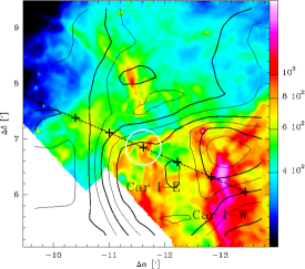
Figure 2: Northern field: Contours of integrated CO 4–3 intensities (cf. Fig. 3) overlayed on 8 $\mu$m IRAC/Spitzer emission in units of MJy/sr. Car I-E and Car I-W are two H ii regions described e.g. by Brooks et al. (2003) (cf. Fig. 3 for more details).

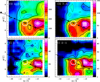
Figure 3: Northern $4^{\prime}\times 4^{\prime}$ field: Velocity-integrated maps of CO 4–3, 7–6, [C i] 1–0, and 2–1 at a common angular resolution of $38^{\prime\prime}$ (0.43 pc), integrated over the full velocity range of emission between $-32$ and $-5$ kms^-1. Contours range between 10 and 90% in steps of 10% of the peak intensities, which are 398 K kms^-1 for CO 4–3, 153 K kms^-1 for CO 7–6, 59 K kms^-1 for [C i] 1–0, and 48 K kms^-1 for [C i] 2–1. The center position of the compact OB cluster Tr 14 is marked by a filled triangle outside the CO 4–3 map. A dashed line and small crosses spaced by $40^{\prime\prime}$ mark a cut through the peak of [C ii] emission (Brooks et al. 2003) (large cross) and Tr 14. The circle marks the resolution and the interface position analyzed in Table 1.

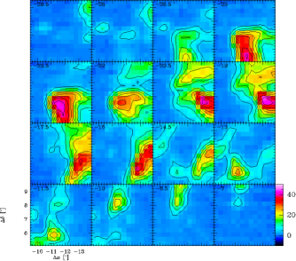
Figure 4: Velocity structure of the northern field: CO 4–3 velocity channels of 1.5 kms^-1 width. Contours range between 5 and 45 K kms^-1 in steps of 5 K kms^-1.

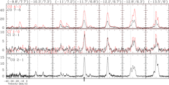
Figure 5: Spectra along a cut through the northern field connecting Tr 14 and the [C ii] peak on a $40^{\prime\prime}$ grid. All data are at a common resolution of $38^{\prime\prime}$ and on the main beam scale. The velocity range is $-40$ to $5$ kms^-1. The dashed vertical lines and the arrow mark the position of the $-24$ kms^-1 velocity component presented in Table 1.

4 Results

4.1 Northern region

4.1.1 Maps of integrated intensities

Figure 2 shows an overlay of integrated CO 4–3 intensities on an 8 $\mu$m image taken with the Infrared Array Camera (IRAC) on the Spitzer space telescope. The 8 $\mu$m data reveal the complicated spatial structure of the region, consisting of several filaments and shell-like structures. The bright region in the south-west is the ionisation front Car I-W. Approximately $\sim 1^{\prime}$ to the east lies Car I-E (cf. Rathborne et al. 2002; Brooks et al. 2001).

Maps of integrated CO 4–3, 7–6, [C i] 1–0, and 2–1 emission (Fig. 3) show the boundary of the northern molecular cloud (orientated north-south) towards the Tr 14 cluster and its H ii region. For all four tracers, the integrated intensities are co-extensive and peak in the south-west, near $-13^{\prime}/+6.5^{\prime}$, i.e. near the peak of [C ii] emission studied by Brooks et al. (2003). The south-eastern interface region exhibits increased CO 7–6 and [C i] 2–1 line intensities, indicating an increased amount of warm, dense gas. The morphology of the cloud resembles a ring centered on a region with less strong emission near $-12^{\prime}/+$6$.\mkern-4.0mu^{\prime}$5. The northern half of the cloud shows weaker and more diffuse emission.

The northern region exhibits a complex velocity structure between $-32$ and $-5$ kms^-1, which can be seen in the CO 4–3 velocity channel maps (Fig. 4). Note that weak CO 4–3 emission is also detected east of the north-south interface, near $-10^{\prime}/+$7$.\mkern-4.0mu^{\prime}$5, at velocities between about $-14.5$ and $-10$ kms^-1. The CO 4–3 emission also corresponds well with the ¹³CO 2–1 SEST channel maps at $25^{\prime\prime}$ resolution shown in Fig. 7 of Brooks et al. (2003). The good correspondance shows that the velocity structure is largely due to individual clumps and not self-absorption of optically thick ¹²CO.

4.1.2 Spectra along a cut through the region

The rich kinematical structure is further revealed by the spectra along a cut, shown in Fig. 5, from the [C ii] emission peak through the cloud interface, towards Tr 14. This cut is orientated the same as the cut presented in Figs. 1 and 11 of Brooks et al. (2003). The spectra of CO 4–3, 7–6, [C i] 1–0, 2–1, and ¹³CO 2–1 (Brooks et al. 2003) show several velocity components with large velocity gradients. At the interface, all tracers show a strong component at $-24$ kms^-1. Further west, this component shifts to lower velocities and splits up into at least 3 components. The line centroids of the different tracers match very well. The peak temperatures are 40 K in CO 4–3 and 10 K in [C i] 1–0. Line intensities of CO and [C i] stay constant within a factor of 2 at the positions within the cloud; they increase slightly at the interface, before dropping rapidly towards the east. A weak component at $-15$ kms^-1 seen in CO and ¹³CO peaks to the east of the interface at ($-$9$.\mkern-4.0mu^{\prime}$8,7$.\mkern-4.0mu^{\prime}$7).

To give one typical example, Table 1 shows the integrated line intensities and derived quantities of the $-24$ kms^-1 component at the interface position, after Gaussian fitting. $T_{\rm ex}$ is derived from the ¹²CO 4–3 peak line temperature assuming optically thick emission and a beam-filling factor of 1. Total CO and C column densities, given in $10^{17}$cm^-2, were derived from ¹³CO 2–1 and [C i] 1–0 assuming optically thin emission at $T_{\rm ex}$, LTE, and a ¹²CO vs. ¹³CO abundance ratio of 65. Total H₂ column densities, given in $10^{21}$cm^-2, and masses were derived from $N$(CO) assuming an abundance ratio of $8.5\,10^{-5}$ (Frerking et al. 1982). C/CO is the abundance ratio $N$(C)/$N$(CO). Errors given for the column densities were derived by varying $T_{\rm ex}$ and the integrated intensities by $\pm 15\%$. While the ¹²CO 4–3 and 7–6 lines show FWHMs of 5.4 and 4.7 kms^-1, the [C i] 1–0 and 2–1 line widths are smaller, 3.9 and 3.1 kms^-1. ¹³CO 2–1 shows a still narrower line width of 2.9 kms^-1. We attribute this change of line widths to optical depth effects. The fitted line center velocities of all tracers agree within 0.5 kms^-1. Line ratios of CO 7–6/4–3 and [C i] 2–1/1–0 are 0.4 and 0.7, which are typical values for the entire cut.

The peak CO 4–3 temperature of 40 K translates, through the Rayleigh-Jeans correction, into a lower limit of the gas kinetic temperature of the emission zone of 50 K. Optical depth effects or a beam-filling factor of less than 1 would imply higher gas kinetic temperatures. Brooks et al. (2003) derived a dust temperature of 50 K from the $60$ vs. $100\,\mu$m IRAS flux ratio at the [C ii] position.

The [C i] 2–1/1–0 line ratio is a sensitive function of the [C i] excitation temperature. In the optically thin limit and assuming LTE, $T_{\rm ex}=38.3\,{\rm K}/\ln[2.11/R_{\rm CI}^{21}]$. At the interface position, we observed a ratio of $0.72\pm 0.15$, assuming a calibration error of the ratio of about 20%. This translates into $T_{\rm ex}$([C i]) of only 35 K(${}^{43\,{\rm K}}_{29\,{\rm K}}$).

The ¹³CO 2–1 spectra (Brooks et al. 2003) peak at 15 K. At the interface, the [C i] 1–0/¹³CO 2–1 ratio is 0.8.

To derive a first estimate of the total CO column densities at the two interface positions (Table 1), we used the ¹³CO 2–1 integrated intensities assuming optically thin emission, LTE, and a ¹²CO vs. ¹³CO abundance ratio of 65. The abundance ratio is in accordance with the average local ISM ¹²C/¹³C ratio of $68\pm 15$ recently found by Milam et al. (2005), which is valid also for Carina at about solar galacto centric distance. The inferred total optical extinction at the northern interface is $28\pm 7$ mag, using the canonical $N$(H₂)/A_v ratio of $9.36\,10^{20}$ cm^-2 mag^-1 (Bohlin et al. 1978). The C/CO abundance ratio is 0.21.

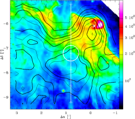
Figure 6: Southern field: Contours of integrated CO 4–3 intensities (cf. Fig. 7) overlayed on 8 $\mu$m IRAC/Spitzer emission in units of MJy/sr.

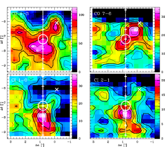
Figure 7: Southern $4^{\prime}\times 4^{\prime}$ field: Velocity-integrated maps of CO 4–3, 7–6, [C i] 1–0, and 2–1 at a common angular resolution of $38^{\prime\prime}$, integrated over the full velocity range of emission between $-20$ and $-32$ kms^-1. Contours range between 10 and 90% in steps of 10% of the peak intensities which are 114 K kms^-1 for CO 4–3, 35 K kms^-1 for CO 7–6, 37 K kms^-1 for [C i] 1–0, and 22 K kms^-1 for [C i] 2–1. A cross $\times$ marks the position of IRAS 10430-5931 at 10$.\!\!^{\rm h}$45$.\!\!^{\rm m}$02$.\!\!^{\rm s}$4 $-59$$.\!\!^{\circ}$47$.\mkern-4.0mu^{\prime}$10$.\!\!^{\prime\prime}$0 (J2000). Small crosses $+$ mark positions along a cut through the interface region. The circle marks the resolution and the position analyzed in Table 1.

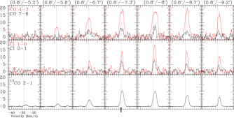
Figure 8: Spectra along a north-south orientated cut through the southern field at $\Delta\alpha=$0$.\mkern-4.0mu^{\prime}$8 on a $40^{\prime\prime}$ grid. All data are at a common resolution of $38^{\prime\prime}$. The velocity range is $-43$ to $-13$ kms^-1. Vertical lines mark a velocity of $-28$ kms^-1. The arrow marks the position analyzed in Table 1.

4.2 Southern region

4.2.1 Maps of integrated intensities

Figure 6 shows an overlay of integrated CO 4–3 intensities on an 8 $\mu$m IRAC/Spitzer image of the southern NANTEN field. The 8 $\mu$m emission traces a sharp interface running from north-east to south-west. It brightens at the cloud edge, showing several elongated filaments and knots along the interface. It also shows a bright emission knob in the north-west, which probably corresponds to the IRAS point source 10430-5931. The 8 $\mu$m, emission here is weaker than in the northern field by about a factor 5. The IRAC emission drops rapidly towards the bulk of the cloud in the south-east, similar to PAH emission traced by the $3.21\,\mu$m image of Rathborne et al. (2002).

In contrast to the mid-infrared emission, CO 4–3 and [C i] integrated intensities (Fig. 7) peak south of the interface deep inside the cloud near ($1^{\prime},-8^{\prime}$). The CO 7–6 line peaks near IRAS 10430-5931, indicating elevated temperatures and densities. In contrast, the IRAS source is not prominent in [C i].

4.2.2 Spectra along a cut through the region

Spectra taken along a north-south cut through the southern field show one component near $-27$ kms^-1 with little variation in velocity (Fig. 8). Near the interface, ¹²CO line profiles are flat-topped indicating high optical depths and self-absorption. Table 1 lists the results of Gaussian fits to the spectra at the interface position (0$.\mkern-4.0mu^{\prime}$8,$-$7$.\mkern-4.0mu^{\prime}$3). The fitted FWHMs are 4.3 kms^-1 (CO 4–3), 3.9 kms^-1 (CO 7–6), 3.4 kms^-1 (¹³CO 2–1), 2.1 kms^-1 ([C i]1–0), 2.4 kms^-1 ([C i]2–1). ¹²CO line widths are a factor $\sim 2$ broader than the [C i] line widths which probably reflects changes of the optical depths.

Compared to the northern field, the ¹²CO and ¹³CO lines are weaker while the [C i] 1–0 line is stronger. The CO 4–3 peaks at only $\sim 20$ K. The line ratios of CO 7–6/4–3 and [C i] 2–1/1–0 at the interface position are $0.3\pm 20\%$ and $0.6\pm 20$% respectively. These ratios are slightly lower than in the northern field, suggesting lower temperatures and densities. However, optical depth effects and self-absorption may also play a role. The [C i] 1–0/CO 4–3 ratio is 0.34 at the interface, a factor 2 higher than in the northern interface. The large-scale survey of the entire Carina region by Zhang et al. (2001) showed variations between 0.14 and 0.45, similar to the ratios we find at angular resolutions which are a factor $\sim 5$ higher. Gas kinetic temperatures must be at least 30 K to explain the ¹²CO 4–3 main beam temperatures. In the southern interface, this is consistent with $T_{\rm ex}$([C i])=30.5 K (${}^{36\,{\rm K}}_{26\,{\rm K}}$) derived from the [C i] line ratio.

The LTE analysis at the southern position indicates a C/CO abundance ratio of 0.26, slightly higher than the abundance ratio in the north. Taking into account the calibration errors, the C/CO abundance ratios lie between $\sim 0.1$ and $\sim 0.4$ at both positions (Table 1). Similar abundance ratios have been observed in other Galactic star forming regions like Cepheus B or NGC 7023 (see references in Mookerjea et al. 2006).

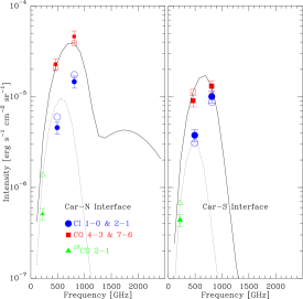
Figure 9: Integrated intensities at the two interface positions in Carina-North and South (Table 1). Filled symbols show the observed ¹³CO 2–1, [C i] 1–0, 2–1, ¹²CO 4–3, and 7–6 intensities. Error bars denote the 15% calibration error. Model results of the best fitting clumpy PDR model (Table 2) are shown by solid (¹²CO) and dotted lines (¹³CO), and open symbols.

Table 2: Parameters of the clump ensembles at the two positions which fit best the observed intensities. Columns (2) to (6) list the input parameters from which the values given in columns (7) to (11) are derived: $\chi$ is the FUV field in Draine units, $\langle n\rangle_{\rm ens}$ is the average density of the clump ensemble, $M_{\rm cl}^{\rm min}$, $M_{\rm cl}^{\rm max}$, $M_{\rm tot}$ are the minimum and maximum clump mass, and the total ensemble mass, respectively. $n_{\rm{0,min}}$ and $n_{\rm{0,max}}$ are the smallest and largest clump surface densities, $R_{\rm min}$ and $R_{\rm max}$ are the smallest and largest clump radii, and $\phi_{A}$ is the beam-filling factor of the clump ensemble.

$\Delta\alpha/\Delta\delta$	$\chi$	$\langle n\rangle_{\rm ens}$	$M_{\rm cl}^{\rm min}$	$M_{\rm cl}^{\rm max}$	$M_{\rm tot}$	$n_{\rm{0,min}}$	$n_{\rm{0,max}}$	$R_{\rm min}$	$R_{\rm max}$	$\phi_{A}$
$(^{\prime},^{\prime})$		cm-3	M⊙	M⊙	M⊙	cm-3	cm-3	pc	pc
(1)	(2)	(3)	(4)	(5)	(6)	(7)	(8)	(9)	(10)	(11)
$-11.7/6.8$	$10^{3.5}$	$2\,10^{5}$	$10^{-2}$	$10^{2}$	400	$5.3\,10^{4}$	$8.8\,10^{5}$	$3.7\,10^{-3}$	$2.1\,10^{-1}$	3.9
$+0.8/-7.2$	$10^{2.5}$	$2\,10^{5}$	$10^{-2}$	$10^{2}$	220	$5.3\,10^{4}$	$8.8\,10^{5}$	$3.7\,10^{-3}$	0.2	2.1

Table 3: Ratios of observed integrated intensities over integrated intensities predicted by the clumpy PDR model. The input parameters used are given in Table 2; deviations from this setting are listed in column (7).

$\Delta\alpha/\Delta\delta$	13CO	CO		[C i]
$(^{\prime},^{\prime})$	2–1	4–3	7–6	1–0	2–1
(1)	(2)	(3)	(4)	(5)	(6)	(7)
$-11.7/6.8$	0.4	1.1	1.2	0.8	0.8
$-11.7/6.8$	0.3	0.9	0.8	0.7	0.8	$M_{\rm min}=10\,^{-3}$ M⊙
$-11.7/6.8$	0.4	1.3	1.7	0.8	1	$M_{\rm min}=10\,^{-1}$ M⊙
$-11.7/6.8$	0.5	1.7	1.5	1.4	1.5	$M_{\rm max}=10^{3}$ M⊙
$-11.7/6.8$	0.3	0.8	1	0.5	0.5	$M_{\rm max}=10^{1}$ M⊙
$+0.8/-7.2$	0.6	0.8	1	1.2	1.2

5 Clumpy interface regions

Figure 9 shows the cooling intensities observed at the two interface positions (Table 1) along the cuts presented in the previous section. At both positions, the 7-6 intensity exceeds the 4-3 intensity. As this transition has a critical density of $1.4\,10^{6}$ cm^-3 and an upper-level energy corresponding to 157 K, temperatures and densities are expected to be similarly high.

In the following, we compare the observed emission with the predictions of a clumpy PDR model (Cubick 2005; Cubick et al. 2007). We assume that the emission stems from an ensemble of spherically symmetric clumps within the beam. The clumps follow the canonical clump mass and mass size distributions: $dN/dM\propto M^{-\alpha}$ and $M\propto R^{\gamma}$. For the clump mass spectrum derived from molecular line observations, $\alpha\sim 1.8$ in a large number of Galactic clouds (e.g. Kramer et al. 1998; Simon et al. 2001). For the power law describing the mass-size distribution, $\gamma\sim 2.3$ in several Galactic clouds (e.g. Heithausen et al. 1998). As a result, the clump density distribution is $n\propto M^{1-3/\gamma}$, i.e. the density increases with decreasing clump mass. For the nearby clouds L 1457 and the Polaris Flare presented in the Kramer and Heithausen papers, the canonical clump mass and mass size distributions continue down to masses of less than $10^{-3}$ M_⊙ and radii of less than $10^{-2}$ pc.

The emission from a clump of given mass and density is calculated by the KOSMA-$\tau$ model (Röllig et al. 2006; Störzer et al. 1996). The radial density structure $n(r)$ of a model clump with radius $R_{0}$ is given by $n(r)\propto n_{0}\,(r/R_{0})^{-1.5}$ for $0.2\leq r/R_{0}\leq 1$ and $n(r)=11.18\,n_{0}=$ const. for $r/R_{0}\leq 0.2$. The clump averaged density $\langle n\rangle$ is about twice the density at the clump surface, called henceforth surface density $n_{0}$: $\langle n\rangle\sim 1.91\,n_{0}$. PDR models of individual clumps were calculated on a grid of FUV fields $\log(\chi)=0,0.5,$ to 6, clump surface densities $\log(n_{0}/{\rm cm}^{-3})=2,2.5,$ to 7, and clump masses $\log(M_{\rm cl}/$M_⊙$)=-3,-2.5,$ to 2. The parameters controlling the ensemble model are the FUV field, the average ensemble density, the total ensemble mass, and the lower and upper clump mass limits. Here, we assume that all clumps are heated by a constant FUV field, as derived from the HIRES observations presented above. We chose a lower mass cutoff of the ensemble of $10^{-2}$ M_⊙ and an upper cutoff of 100 M_⊙. Below, we show that the exact choice of these limits does however not have a strong impact on the resulting model intensities (cf. Cubick et al. 2007). To fit the observed intensity ratios [C i] 2–1/1–0 and CO 7–6/4–3, the only free parameter is then the average density of the clump ensemble $\langle n\rangle_{\rm ens}$.

We adapted the total ensemble mass to fit the absolute intensities. The best fitting models and their parameters are shown in Figure 9 and in Table 2. Table 3 lists the ratios of observed over modelled intensities for all 5 observed transitions. For a perfectly fitting model, they would all equal $1\pm 15\%$, reflecting the estimated calibration error of the observed data.

Northern interface.

An average ensemble density of $2\,10^{5}$ cm^-3 allows us to reproduce the observed ¹²CO 7–6/4–3 and [C i] 2–1/1–0 line ratios very well at the northern interface position. Lower densities do not reproduce the high CO 7–6/4–3 line ratios, but rather lead to a peak of the cooling curve at $J\leq 5$. The absolute intensities of the ¹²CO and ¹²C lines can be reproduced to within 20% for an ensemble mass of 400 M_⊙. The strongest deviation occurs for ¹³CO; the observed ¹³CO 2–1 line intensity is only 40% of the modelled intensity.

The geometrical beam-filling factor of the clump ensemble is defined as the ratio of the sum of all clump areas over the beam area, i.e. $\phi_{A}=\Omega_{\rm ens}/\Omega_{\rm beam}$, with $\Omega_{\rm ens}=\sum\pi R_{\rm cl}^{2}/d^{2}$ at distance $d$. The beam-filling factor is 3.9 at the northern interface position (Table 2). We assume that clumps don’t overlap, i.e. that their emission escapes without being absorbed by foreground clumps, and there is no interclump medium. Clumps have a constant velocity FWHM of $\Delta{\rm v}=1.7$ kms^-1. The clumpy ensemble models developed by Cubick et al. (2007) do not yet predict line profiles. Table 2 gives the densities and radii of the smallest and largest clumps of the ensemble. The mass of the smallest clump is set to $10^{-2}$ M_⊙. The virial mass of the smallest clump, $M_{\rm vir}\propto R\Delta{\rm v}^{2}$ is a factor 400 larger. In other words, the velocity width of these clumps are far too large for pure gravitational virialization. The external pressure which would be needed to confine these clumps, $10^{8}$ Kcm^-3, is far too large to be maintained by an interclump medium. The large ratio indicates instead that these clumps, if they do exist, are transient features of the turbulent gas and evaporating on very short time scales: $t_{\rm evap}\approx R/\sigma_{\rm v}=R/{\rm FWHM}\sqrt{8\ln 2}\approx 5000\,$yrs.

The modelled intensities depend only weakly on the lower and upper mass limits of the ensemble as shown in Table 3. Varying one of the mass limits by one order of magnitude while keeping all other 4 input parameters listed in Table 2 unchanged, the absolute intensities of the 5 transitions vary by less than a factor of $\sim 2$ relative to the best fitting solution. This is discussed in more detail in Cubick et al. (2007).

The run of ¹²CO intensities with rotational number $J$, i.e. the CO cooling curve, predicted by the model (Fig. 9) shows a maximum at $J=7$ and a steep drop at higher rotational numbers up to $J=11$ by more than a magnitude. A secondary peak of the cooling curve is seen at $J=15$; it is almost a factor 10 weaker than the first maximum. The second peak shows up only for FUV fields above $\sim 10^{3}$ and it stems predominantly from the surface regions of the small, dense clumps. These clumps are large in number, have a large total surface area, which is heated to high temperatures, sufficient to excite these high-$J$ lines. The abundance of CO is increased in the hot gas of the H i/H₂ surface layer, near the OH density peak, due to secondary production paths which become important at high temperatures (Sternberg & Dalgarno 1995):

$${\rm OH}+{\rm C}^{+} \rightarrow {\rm CO}+{\rm H}^{+}\hskip 14.22636pt{\rm(R13)}$$

$${\rm OH}+{\rm C}^{+} \rightarrow {\rm CO}^{+}+{\rm H}\rightarrow{\rm CO}+{\rm H}^{+}\hskip 14.22636pt{\rm(R125,R126)}$$

$${\rm CO}^{+}+{\rm H}_{2} \rightarrow {\rm HCO}^{+}+{\rm H}\hskip 14.22636pt{\rm(R127)}$$

$${\rm HCO}^{+}+e \rightarrow {\rm CO}+{\rm H}\hskip 14.22636pt{\rm(R129)}$$

We suspect that these reactions lead to the secondary peak of the cooling curve shown in Figure 9.

Southern interface.

At the southern interface position, the FUV field is only $10^{2.5}\,\chi_{0}$. An average ensemble density of $2\,10^{5}$ cm^-3 reproduces the observed ¹²CO 7–6/4–3 and [C i] 2–1/1–0 line ratios. Within 40%, the clumpy model is also consistent with the absolute intensities of all 5 tracers for a total ensemble mass of 220 M_⊙ (Fig. 9, Tables 3,2). Due to the weaker FUV field compared to the northern position, the CO cooling curve peaks at slightly lower frequencies and a second peak is not visible. Similar to the northern position, the strongest deviation occurs for the ¹³CO 2–1 lines.

6 Summary

We have mapped the emission of atomic carbon and CO in two fields of the GMCs surrounding $\eta$Car. Combining CO 4–3 and [C i] 1–0 data with CO 7–6 and [C i] 2–1 data allows us to study the excitation conditions of both gas tracers. The northern $4^{\prime}\times 4^{\prime}$ field lies adjacent to the compact OB cluster Tr 14 and is associated with the H ii regions Car I-E and Car I-W. The spectral lines show a rich kinematical structure, with several velocity components along the lines of sight spread between $-10$ and $-30\,$kms^-1. The southern $4^{\prime}\times 4^{\prime}$ field lies on a molecular ridge south of $\eta$Car. Here, spectral lines show only one rather narrow Gaussian shaped velocity component. The FUV field derived from HIRES/IRAS far-infrared data is $\chi\sim 10^{2.5}$, about a factor 10 weaker than in the northern field. IRAC/Spitzer maps at 8$\mu$m show the detailed structure of the FUV illuminated dust. The edge of the southern region is clearly delineated by the $8\mu$m emission, while the northern region shows a more complex spatial structure.

In both regions, CO and [C i] emission is co-extensive. Both species appear to trace the bulk of molecular gas, rather than the interface regions. This coincidence has been found in many of the previous large-scale studies of Galactic clouds conducted with the Mt.Fuji, KOSMA, and other telescopes. Papadopoulos et al. (2004) stress the importance of cosmic rays in raising the C/CO abundance ratio and argue that dynamic and non-equilibrium chemistry processes explain the ubiquity of [C i] within molecular clouds as well as at PDR interfaces. Here, we argue that steady state, clumpy PDR models provide an alternative explanation.

The northern and southern Carina regions both show a slight brightening of the CO 7–6 and [C i] 2–1 transitions relative to the 4–3 and 1–0 transitions near the interfaces. In the south-east part of the northern region, the upper transitions brighten towards the interface (Fig. 3). These transitions also show increased intensities near the embedded IRAS point source in the southern region (Fig. 7).

We selected two cuts from the cloud cores through the interface regions, roughly pointing towards the illuminating sources. The southern cut lies to the east of IRAS 10430-5931, avoiding its complicated structure and additional heating sources. The northern cut runs from the peak of [C ii] emission (Brooks et al. 2003) through the H ii regions Car I-W and I-E across the edge-on interface towards the center of the Tr 14 cluster.

The peak ¹²CO line temperatures along the northern cut indicate kinetic gas temperatures of at least 50 K, while a lower limit of 30 K is found along the southern cut.

We selected two positions at the northern and southern interfaces for a detailed analysis. The ¹²CO 7–6/4–3 and [C i] 2–1/1–0 intensity ratios at these positions are 0.3–0.4 and 0.6–0.7, respectively. We use PDR models to interpret the observed line intensities. Our models assume that all observed emission stems from an ensemble of spherically symmetric PDR clumps and there is no emission from an interclump medium or a diffuse halo surrounding the clouds. PDR clumps are modelled using the stationary KOSMA-$\tau$ code (Röllig et al. 2006). The clump distributions follow the canonical mass and radius distributions found for molecular clouds. At the two positions analyzed in detail, we find that clumpy PDR models are consistent with the observed absolute intensities of the ¹²CO and [C i] lines to within 20%, i.e. at about the calibration accuracy.

Since the line ratios observed at the two interface positions are fairly typical for the entire observed regions, we conclude that stationary, clumpy PDR models can simultaneously reproduce the observed [C i] and CO emission of the lower transitions and the upper CO 7–6 and [C i] 2–1 transitions.

However, the observed ¹³CO 2–1 intensities are only about half of the modelled intensities at the northern and southern positions, respectively. Interestingly, Pineda & Bensch (2007) report a similar finding. They analyzed ¹²CO and [C i] emission observed in the dark cloud globule B 68. This emission can be reproduced using a single KOSMA-$\tau$ spherically symmetric PDR model, while the observed ¹³CO intensities are a factor $\sim 2$ too low.

To study the gas under a broad range of conditions, we plan to extend the present [C i] and CO maps to fully cover the GMCs surrounding $\eta$Car using the SMART 492/810 GHz multipixel array receiver at NANTEN2 (Graf et al. 2003). Future observations with APEX and Herschel will tell in how far the emission of other species tracing the detailed photo-chemical network is also consistent with stationary, clumpy PDR models.