Renormalization group study of transport through a superconducting
junction of multiple one-dimensional quantum wires

Abstract

We investigate transport properties of a superconducting junction of many ($N\geq 2$) one-dimensional quantum wires. We include the effect of electron-electron interaction within the one-dimensional quantum wire using a weak interaction renormalization group procedure. Due to the proximity effect, transport across the junction occurs via direct tunneling as well as via the crossed Andreev channel. We find that the fixed point structure of this system is far more rich than the fixed point structure of a normal metal$-$superconductor junction ($N=1$), where we only have two fixed points - the fully insulating fixed point or the Andreev fixed point. Even a two wire ($N=2$) system with a superconducting junction i.e.  a normal metal$-$superconductor$-$normal metal structure, has non-trivial fixed points with intermediate transmissions and reflections. We also include electron-electron interaction induced back-scattering in the quantum wires in our study and hence obtain non-Luttinger liquid behaviour. It is interesting to note that (a) effects due to inclusion of electron-electron interaction induced back-scattering in the wire, and (b) competition between the charge transport via the electron and hole channels across the junction, give rise to a non-monotonic behavior of conductance as a function of temperature. We also find that transport across the junction depends on two independent interaction parameters. The first one is due to the usual correlations coming from Friedel oscillations for spin-full electrons giving rise to the well-known interaction parameter (${{\alpha=(g_{2}-2g_{1})/2\pi\hbar v_{F}}}$). The second one arises due to the scattering induced by the proximity of the superconductor and is given by (${{\alpha^{\prime}=(g_{2}+g_{1})/2\pi\hbar v_{F}}}$). The non-monotonic conductance and the identification of this new interaction parameter are two of our main results. In both the expressions ${{g_{1}=V(2k_{F})}}$, ${{g_{2}=V(0)}}$, where $V(k)$ is the inter electron interaction potential.

I Introduction

Effects due to the proximity of a superconductor has motivated a lot of work andreev ; blonder ; beenaker in the last several decades. A direct manifestation of proximity effect is the phenomenon of Andreev reflection (AR) in which an electron like quasi-particle incident on normal$-$superconductor (NS) junction is reflected back as a hole along with the transfer of two electrons into the superconductor as a Cooper pair. An even more intriguing example where the proximity effect manifests itself is the phenomenon of crossed Andreev reflection (CAR) which can only take place in a normal metal$-$superconductor$-$normal metal (NSN) junction provided the distance between the two normal metals is less than or equal to the phase coherence length of the superconductor. This is a nonlocal process where an incident electron from one of the normal leads pairs up with an electron from the other lead to form a Cooper pair byers ; feinberg ; exp ; hekking1 ; hekking2 and joins the superconductor. Its relevance in the manipulation of spin currents drsahaepl (SC) and questions regarding production of entangled electron pairs in nano devices for quantum computation has attracted a lot of attention in recent times buttiker1 ; buttiker2 ; buttiker3 ; recher ; bouchiat ; beckmann ; russo ; chandrasekhar ; yeyati . Further extensions such as inclusion of effects due to electron-electron interactions on AR processes in case of NS junctions in the context of one-dimensional (1–D) wires have also been considered recently jap1 ; jap3 ; fazio ; bena ; man ; titov .

In this article, we shall first develop a general formulation for studying the transport properties of a multiple quantum wire (QW) junction in the spirit of the “Landauer–Buttiker” approach landauer , where the junction itself is superconducting. We shall use this formulation to study the influence of the proximity effect on the transport properties of a superconducting junction specifically for the case of two and three 1–D interacting quantum wires and show how the simple case of junction of a single 1–D QW with a superconductor (NS junction) is different from the multiple wire junction counterpart. Because of the existence of the AR process, both electron and hole channels take part in transport. The power law dependence of the Andreev conductance for the NS junction case was first obtained using weak interaction renormalization group (WIRG) approach by Takane and Koyama in Ref. jap1, . This was in agreement with earlier results from bosonization jap3 , which, however,

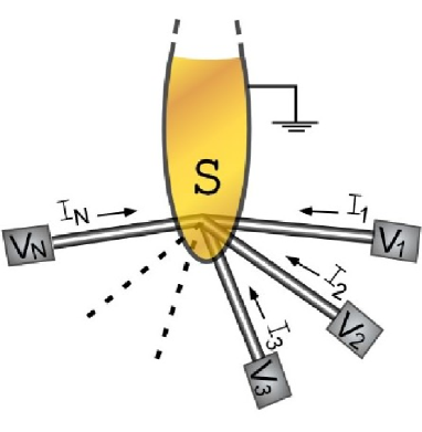
Figure 1: Multiple wires connected to a superconducting junction. The dashed lines represents the fact that the model can be trivially extended to more than two wires. ‘$a$’ is the effective length of the superconductor.

could only handle perturbative analyses around the strong back-scattering (SBS) and weak back-scattering (WBS) limits. The WIRG approach, on the other hand, can study the full cross-over from WBS limit to SBS limit. Hence the WIRG approach is very well-suited for studying problems where the aim is to look for non trivial fixed points with intermediate transmissions and reflections. This would be difficult using a bosonization approach.

For the NS junction case, it was shown that the power law exponent for the temperature dependence of conductance was twice as large as the exponent for a single barrier in a QW. This happens because of the introduction of the extra hole channel due to AR. The WIRG approach takes into account both (a) electron-electron interaction induced forward scattering processes which gives standard Luttinger liquid behavior, and (b) electron-electron interaction induced back-scattering processes which give rise to non Luttinger liquid behavior (deviation from pure power law behavior) as obtained by Matveev  et al.   in Refs. matveev, and yue, . The most interesting point to be noticed here is the fact that both bosonization and WIRG give the same Luttinger liquid power law dependence for the conductance of NS junction although the WIRG approach actually takes into account the extra process of electron-electron back-scattering which usually leads to non Luttinger liquid behavior. This happens because there is a remarkable cancellation in perturbation theory which nullifies any deviation from pure power law behavior of conductance.

In this article, we show that this kind of cancellation does not happen for the NSN junction or for that matter, for any junction comprising of more than two 1–D quantum wires. Hence, deviations from pure power law do exist. We show that due to the inter-play of the proximity and the interaction effects, one gets a novel non-monotonic behavior of conductance for the case of NSN junction as a function of the temperature. Note that this is something which cannot be obtained in a bosonization analysis which neglects the back-scattering part of the electron-electron interaction. We extend our results to junctions with a ferromagnetic wire on one side, i.e., ferromagnet–superconductor–normal (FSN) junctions and to junctions with ferromagnets on both sides, i.e., ferromagnet–superconductor– ferromagnet (FSF) junctions. Here we assume that the influence of the junction between the superconductor and the ferromagnetic wire has a very small effect on the spectrum of the superconductor itself. Of course this is true only if the superconductor is large enough. We also study transport through a superconductor at the junction of three wires (and finally extend it to N wires). This generalizes the earlier work on junctions lal ; das to also include proximity effects.

In Sec. II, we review the applicability and strength of the WIRG approach when applied to quantum impurity problems, such as, a normal junction of multiple quantum wires, or a junction with a spin impurity. Then we discuss how one can apply the WIRG technique to the problem studied in this paper. In Sec. III, we describe the set-up for our system, i.e.  a superconductor at the junction of N wires, in terms of a scattering matrix and briefly discuss the symmetries of the proposed model. We then perturbatively (in electron-electron interaction strength) calculate the leading order logarithmic corrections to both the normal reflection amplitude and the AR amplitude which, in turn, give corrections to the conductance via the Landauer–Buttiker formula. In Sec. IV, we obtain the RG equation for the NS junction and reproduce the known fixed points using our approach. Then we derive the RG equation for the symmetric NSN junction and obtain the RG flow between various fixed points and analyse the results of the study. Unlike, the renormalization group flow of the NS junction, which does not lead to any non-monotonicity, we show that the inclusion of the CAR and direct tunneling through the superconductor gives rise to a non-monotonic conductance as a function of the temperature. In Sec. V, we present our results for specific cases of NSN . In Sec. VI, we study the three$-$wire$-$superconducting$-$junction and show the existence of a fixed point which is analogous to the Griffith’s fixed point lal ; das in the three$-$wire$-$normal$-$junction case. Finally in Sec. VII, we present our summary and discussions.

II WIRG vis-a-vis Bosonization

Transport through a quantum scatterer (for instance, a simple static barrier or a dynamical impurity like Kondo spin) in a 1–D interacting electron gas is qualitatively different from its higher dimensional counterpart k&f . This is because, in 1–D, due to electron-electron interactions, the Fermi-liquid ground state is destroyed and the electrons form a non-Fermi liquid ground state known as as Luttinger Liquid haldane . The low energy dynamics of the 1–D system is governed mainly by coherent particle-hole excitations around the left and the right Fermi points. It is natural to use bosonic fields to describe these low lying excitations. This can be done by re-expressing the original fermions using boson coherent state representation usds ; vondelft ; solyom which is referred to as bosonization. But this approach only allows for a perturbative analysis for transport around the limiting cases of SBS and WBS for the quantum impurity problem. On the other hand, if we start with a very weakly interacting electron gas, it is possible to do a perturbative analysis in the electron-electron interaction around the free fermion Hamiltonian, but treating the strength of the quantum impurity exactly. This allows us to study transport through the impurity for any scattering strength. The strength of this approach lies in the fact that even in presence of electron-electron interaction, one can use single particle notions such as the transmission and reflection amplitudes in order to characterize the impurity. The idea is to calculate correction to transmission and reflection amplitude perturbatively in the interaction strength. Of course, since we are working in 1–D, the perturbative correction turns out to be logarithmically divergent. To obtain a finite result, one has to sum up all such divergent contributions to the transmission and reflection amplitudes to all relevant orders at a given energy scale. This was first done by Matveev  et al.   in Refs. matveev, and yue, in the context of a single (scalar) scatterer for both spin-less and spin-full electrons using the “poor man’s scaling” approach anderson . In the spin-less case, it was shown that the logarithmic correction to the bare transmission amplitude (to first order in interaction parameter parameterized by $\alpha$) was ${{\delta T=2\,\alpha\,T_{0}\,\left(1\,-\,T_{0}\right)\,{\ln}(kd)}}$ and the explicit RG equation for transmission probability was $dT/dl=-2\alpha T(1-T)$ where $k$ was the momentum of the fermion measured from $k_{F}$, $d$ was a short distance cut-off and $\alpha$ was the interaction parameter given by $\alpha=\alpha_{1}-\alpha_{2}$ with $\alpha_{1}={{V(0)}/{2\pi\hbar v_{F}}}$ and $\alpha_{2}={V(2k_{F})}/{2\pi\hbar v_{F}}$. The RG equation upon integration gave the transmission probability as,

$$T(L)={\displaystyle\frac{T_{0}e^{-2\alpha l}}{\left[{1-T_{0}+T_{0}e^{-2\alpha l}}\right]}}={\displaystyle\frac{T_{0}\left(\frac{d}{L}\right)^{2\alpha}}{\left[1-T_{0}+T_{0}\left(\frac{d}{L}\right)^{2\alpha}\right]}}$$ (1)

Here, $l=-\ln(kd)=\ln({L/d})$ where $L$ is the length scale. $l$ can also be measured as a function of the temperature by introducing the thermal length, $L_{T}=({\hbar v_{F}})/({k_{B}T})$. $T_{0}$ is the bare transmission at the short distance cut-off, $d$. It is easy to see from Eq. 1 that for very small values of $T_{0}$, $T_{0}$ can be neglected in the denominator of the expression for $T(L)$ leading to a pure power law scaling consistent with the power law known from bosonization in the WBS limit. Similarly for the spin-full electrons, it was shown that the parameter $\alpha$ in the power law gets replaced by a new parameter, $\beta$ given by $\beta={(g_{2}-2g_{1})}/{\pi\hbar v_{F}}$ where $g_{2}=g_{2}(k)$ and $g_{1}=g_{1}(k)$ are momentum dependent functions or “running coupling constants”. The momentum dependence of $\beta$ here is in sharp contrast to the momentum independent $\alpha$ in the spin-less case. At high momentum, (or equivalently, at the short distance cut-off scale), $g_{1}(d)=V(2k_{F})$ and $g_{2}(d)=V(0)$. Because of the extra logarithmic dependence coming from scaling of the interaction parameter itself (see Eq. 3 and Eq. LABEL:intrg2 below), the expression for transmission matveev ; yue , no longer shows a pure power law scaling even for small values of $T_{0}$. Instead $T(L)$ is now given by

$$T(L)={\displaystyle\frac{\left[T_{0}\left[1+\alpha_{1}\ln\left(\frac{L}{d}\right)\right]^{\frac{3}{2}}\left(\frac{d}{L}\right)^{(2\alpha_{2}-\alpha_{1})}\right]}{\left[1-T_{0}+T_{0}\left[1+2\alpha_{1}\ln\left(\frac{L}{d}\right)\right]^{\frac{3}{2}}\left(\frac{d}{L}\right)^{(2\alpha_{2}-\alpha_{1})}\right]}}$$ (2)

using the length scale dependence of $g_{1}(L)$ and $g_{2}(L)$ given by solyom

$$g_{1}(L) = {\displaystyle\frac{V(2k_{F})}{\left[1+\frac{V(2k_{F})}{{\pi v_{F}}}\ln(\frac{L}{d})\right]}}$$ (3)

$$g_{2}(L) = V(0)-\frac{1}{2}\,V(2k_{F})+\frac{1}{2}\,{\displaystyle\frac{V(2k_{F})}{\left[1\,+\,\frac{{V(2k_{F})}}{{\pi v_{F}}}\ln(\frac{L}{d})\right]}}$$

Note that in the absence of electron-electron interaction induced back-scattering (i.e., when $V(2k_{F})=0$), there is no correction to the power law behavior. Hence, bosonization, which ignores electron-electron back-scattering always results in power law behaviour. But, when electron-electron interaction induced back-scattering is included, the sign of $g_{2}-2g_{1}$ can change under RG flow, and hence, there can be a qualitative change in the behavior of the conductance. The conductance actually develops a non-monotonic dependence on the temperature; it first grows and then drops to zero. But, except for this non-monotonic behavior of conductance for the spin-full case, there is no new physics which is found by studying the full crossover from WBS to SBS. In conclusion, both bosonization and WIRG methods predict that for the single scatterer problem there are only two fixed points - (a) the perfectly back-scattering (no transmission) case is the stable fixed point and (b) the no back-scattering (perfect transmission) case is the unstable fixed point. There are no fixed points with intermediate transmission.

It was first shown by Lal  et al.  in Ref. lal, , using the WIRG approach that even though there are only two fixed points for the two$-$wire$-$junction, surprisingly enough, the three$-$wire$-$junction has a host of fixed points, some of which are isolated fixed points while others are one parameter or multi parameter families of fixed points. It was also shown to be true for more than three wires. From this point of view, the physics of a two$-$wire$-$junction is different from its three$-$wire$-$counterpart. The three$-$wire$-$junction was also studied using bosonization and conformal field theory methods nayak ; affleck1 ; affleck2 ; das2 , which confirmed some of the fixed points found using WIRG. It also gave some extra fixed points which were related to charge fractionalisation at the junction, and which could not be seen within the WIRG approach. The WIRG method was further extended to complicated systems made out of junctions of QW which can host resonances and anti-resonances in Ref. das, . The scaling of the resonances and anti-resonances were studied for various geometries which included the ring and the stub geometry. In particular, it was shown that for a multiple$-$wire$-$junction, the RG equations for the full $S$-matrix characterizing the junction take a very convenient matrix form,

$${\displaystyle\frac{dS}{dl}}=-(SF^{\dagger}S~{}-~{}F)$$ (5)

where $S$ is the scattering matrix at the junction and $F$ is a diagonal matrix that depends on the interaction strengths and the reflection amplitude in each wire. The advantage of writing the RG equation this way is that it immediately facilitates the hunt for various fixed points. All one needs to do is to set the matrix on the LHS of Eq. 5 to zero. This will formally provide us with all the fixed points associated with a given $S$-matrix. This approach was further extended in Refs. ravi1, ; ravi2, to study the multiple$-$wire$-$junction with a dynamical scatterer, i.e.  a (Kondo) spin degree of freedom. The coupled RG equations involving the Kondo couplings, $J_{ij}$ as well as the $S$-matrices were solved. For different starting scalar $S$-matrices, the RG flows of the Kondo couplings was studied. The temperature dependence of the conductances was shown to have an interesting interplay of the Kondo power laws as well as the interaction dependent power laws. Finally, the WIRG method was also extended to the case of NS junction jap1 ; jap3 . In the vicinity of the superconductor, it is well-known that the system is described by holes as well as electrons degennes . Hence the $S$-matrix characterizing the junction not only includes the electron channel but also the hole channel. Naively, one might expect that in the presence of particle-hole symmetry, the only effect of including the hole channel would be to multiply the conductance by a factor of two (in analogy with inclusion of spin and imposing spin up-spin down symmetry). However, it was shown jap1 ; jap3 that in the vicinity of a superconductor, the proximity induced scattering potential that exists between electron and holes, also gets renormalized by electron-electron interactions. When this scattering is also taken into account, the correction to the scattering amplitude to first order in the interaction parameter depends on $(2g_{2}-g_{1})$ instead of $(g_{2}-2g_{1})$. It is worth stressing that this particular linear combination of the interaction parameters ($g_{i}$’s) is independent of the scaling as the logarithmic factors ($l=\ln(kd)$) in Eqs. 3 and LABEL:intrg2 cancel each other. Hence, there is no non-monotonic behavior of the conductance in this case. The WIRG predicted only two fixed points, the Andreev fixed point (perfect AR) which turns out to be an unstable one and the perfectly reflecting fixed point which is the stable fixed point. The NS junction has also been studied using bosonizationjap2 . It is easy to check that the power laws resulting from bosonization agree with those obtained from the WIRG , when the electron-electron interaction induced back-scattering ( which is dropped in the bosonization method) is ignored.

In this article, we apply the WIRG method to the superconducting junction of multiple quantum wires. We note that we now have two complications - (a) multiple wires are connected to the junction and (b) we have both electron and hole channels connected to the junction. So in this case, even for the NS junction, we have two spin channels as well as the electron and hole channels, so the scattering matrix is four component. For $N$ wires, the scattering matrix is $4N\times 4N$-dimensional. Although, we expect our method to work well even in this case, there is one caveat we must keep in mind. We have incorporated the effect of the superconductor as a boundary condition on the QW and neglected any internal dynamics of the superconductor itself. This should work reasonably well as long as we are studying transport at energies much below the superconducting gap. Our main result here is that the conductance across the junction depends on both $g_{1}$ and $g_{2}$ and not on a a special combination $2g_{2}-g_{1}$ (as in NS case) which does not get renormalized under RG flow.Hence, the cancellation of the logarithmic terms in the effective interaction parameter is specific to the NS case and is not true in general. For $N\geq 2$ wires attached to a superconductor, we expect a non-monotonic form of the conductance. We also expect to get a host of fixed points with intermediate transmission and reflection, knowledge of which can be of direct relevance for application to device fabrication of such geometries.

III Superconducting junction with $N$ quantum wires

Let us consider multiple ($N$) quantum wires meeting at a junction on which a superconducting material is deposited as depicted in Fig. 1. The wires are parameterized by coordinates $x_{i}$, with the superconducting junction assumed to be at $x_{i}=0$. We consider a situation where the effective width ‘$a$’ of the superconductor between two consecutive wires is of the order of the phase coherence length of the superconductor (size of the Cooper pair). For our purpose, it is safe to ignore the finiteness of ‘$a$’ and effectively treat the junction of QW as a single point in space with an appropriate boundary condition. We parameterize the junction by the following quantum mechanical amplitudes. There are two kinds of reflection amplitudes: the normal reflection amplitude ($r_{ii\,s_{i}\,s_{i}}$) and the AR amplitude ($r_{A{ii}\,s_{i}\,s_{i}}$) on each wire. In addition, there are two kinds of transmission amplitudes between different wire: the co-tunnelling (CT) amplitude ($t_{ij\,s_{i}\,s_{j}}$) and the CAR amplitude ($t_{Aij\,s_{i}\,s_{j}}$). The indices $s_{i},s_{j}$ refer to the spin of incoming and outgoing particles. As we consider a singlet superconductor at the junction, spin remains conserved in all the processes mentioned above. Thus, the boundary conditions are parametrized by a $4N\times 4N$ scattering matrix for $N$ quantum wires connected to a superconducting junction.

Let us now consider the various symmetries that can be imposed to simplify the $4N\times 4N$ matrix. We impose particle-hole symmetry, i.e., we assume that the reflection and transmissions are the same for particles (electrons) and holes. Further, in the absence of a magnetic field, spin symmetry is conserved which implies that the various transmission and reflection amplitudes for spin up-down electrons and holes are equal. (This symmetry breaks down in the presence of magnetic fields, or in the case of ferromagnetic wires). Also, since we assume that all the wires, connected to the superconductor, are indistinguishable, we can impose a wire index symmetry. (This symmetry again can be broken if we take some ferromagnetic and some normal wires attached to the superconductor). On imposing these symmetries, the $S$-matrix for a two-wire system is given by

$$S\quad=\quad\begin{vmatrix}~{}S_{\uparrow}&0~{}\\ ~{}0&S_{\downarrow}~{}\end{vmatrix}$$

with

$$S_{\uparrow}\quad=\quad S_{\downarrow}\quad=\quad\begin{vmatrix}~{}r&t&r_{A}&t_{A}~{}\\ ~{}t&r&t_{A}&r_{A}~{}\\ ~{}r_{A}&t_{A}&r&t~{}\\ ~{}t_{A}&r_{A}&t&r~{}\end{vmatrix}$$ (6)

Here $r$ stands for normal reflection of electron or hole in each wire, and $r_{A}$ represents AR from electron to hole or vice-versa in each wire. $t$ represents the elastic CT amplitude ($t=t_{12}=t_{21}$) while $t_{A}$ represents the CAR amplitude ($t_{A}=t_{A12}=t_{A21}$). For the spin symmetric case, there are two such matrices, one for spin up electrons and holes and one for spin down electrons and holes. Note that this is the relevant $S$-matrix at energy scales (temperature and applied voltage on the wires) $k_{B}\,T,eV_{i}\ll\Delta$, where $\Delta$ is the superconducting gap energy. The competition between CT and CAR has been analysed before hekking1 ; hekking2 and also different ways of separating the contributions experimentally have been considered beckmann . However, the effect of electron-electron interactions within the wires has not been considered for the NSN case. It is worth emphasizing here that if such NSN junctions are made out of 1–D systems like carbon nanotubes, then the effect of electron-electron interactions can influence the low energy dynamics significantly.

The Landauer$-$Buttiker conductance matrix for the NSN case can be written, in the regime where $k_{B}\,T,eV_{i}\ll\Delta$, as hekking1

$$\begin{vmatrix}~{}I_{1}~{}\\ ~{}I_{2}~{}\\ \end{vmatrix}~{}=~{}\begin{vmatrix}~{}G_{A}+G_{CA}+G_{CT}&G_{CA}-G_{CT}~{}\\ ~{}G_{CA}-G_{CT}&G_{A}+G_{CA}+G_{CT}~{}\end{vmatrix}\begin{vmatrix}~{}V_{1}~{}\\ ~{}V_{2}~{}\end{vmatrix}$$ (7)

The conductances here are related to the elements of the $S$-matrix: $G_{A}\propto|r_{A}|^{2}$, $G_{CT}\propto|t|^{2}$ and $G_{CA}\propto|t_{A}|^{2}$. $G_{A}$ is the conductance due to the AR that occurs at a single NS junction, whereas $G_{CT}$ and $G_{CA}$ are the conductance due to the elastic CT and CAR processes respectively, both of which involve transmissions between two wires and give contributions with opposite signs to the sub-gap conductance between the two wires, $G_{CA}-G_{CT}$ . The generalization of this to $N>2$ is straightforward, and some details are presented in Sec. VI.

IV WIRG study of junctions

We study the effects of inter-electron interactions on the $S$-matrix using the renormalization group (RG) method introduced in Ref. yue, , and the generalizations to multiple wires in Refs. lal, ; das, . The basic idea of the method is as follows. The presence of back-scattering (reflection) induces Friedel oscillations in the density of non-interacting electrons. Within a mean field picture for the weakly interacting electron gas, the electron not only scatters off the potential barrier but also scatters off these density oscillations with an amplitude proportional to the interaction strength. Hence by calculating the total reflection amplitude due to scattering from the scalar scatterer and from the Friedel oscillations created by the scatterer, we can include the effect of electron-electron interaction in calculating transport. This can now be generalized to the case where there is, besides non-zero reflection, also non-zero AR .

To derive the RG equations in the presence of Andreev processes, we will follow a similar procedure to the one followed in Ref. lal, . The fermion fields on each wire can be written as,

$$\psi_{is}(x)=\Psi_{I\,is}(x)\,e^{i\,k_{F}\,x}\,+\,\Psi_{O\,is}(x)\,e^{-i\,k_{F}\,x}$$ (8)

where $i$ is the wire index, $s$ is the spin index which can be $\uparrow,\downarrow$ and $I,O$ stands for outgoing or incoming fields. Note that $\Psi_{I}(x)(\Psi_{O}(x))$ are slowly varying fields on the scale of $k_{F}^{-1}$ and contain the annihilation operators as well as the slowly varying wave-functions. For a momentum in the vicinity of $k_{F}$, the incoming and outgoing fields (with the incoming field on the $i^{th}$ wire) can be Fourier expanded in a complete set of states and the electron field can be written as

$$\Psi_{is}(x) = \int~{}dk~{}\Big{[}\,b_{ks}\,e^{i\,(k\,+\,k_{F})\,x}\,+\,d_{ks}^{\dagger}\,e^{i\,(-k\,+\,k_{F})\,x}$$

$$+ r\,b_{ks}\,e^{-i\,(k\,+\,k_{F})\,x}\,+\,r^{\star}\,d_{ks}^{\dagger}\,e^{-i\,(-k\,+\,k_{F})\,x}$$

$$+ r_{A}\,d_{ks}\,e^{-i\,(-k\,+\,k_{F})\,x}\,+\,r_{A}^{\star}\,b_{ks}^{\dagger}\,e^{-i\,(k\,+\,k_{F})\,x}\Big{]}$$

$$\Psi_{(j\neq i)s}(x) = \int~{}dk~{}\Big{[}tb_{ks}\,e^{i\,(k\,+\,k_{F})\,x}\,+\,td_{ks}^{\dagger}\,e^{i\,(-k\,+\,k_{F})\,x}$$

$$+ t_{A}\,d_{ks}\,e^{-i\,(-k\,+\,k_{F})\,x}\,+\,t_{A}^{\star}\,b_{ks}^{\dagger}\,e^{-i\,(k\,+\,k_{F})\,x}\Big{]}$$

where $b_{ks}$ is the electron destruction operator and $d_{ks}$ is the hole destruction operator. Note that we have chosen to quantize the fermions in the basis of the space of solutions of the Dirac equation, in the presence of a potential which allows for normal as well as Andreev scattering. We have also allowed for both incident electrons and holes. We find that (dropping a constant background density),

$$\langle~{}\rho_{is}(x)~{}\rangle=\langle~{}\Psi_{is}^{\dagger}\Psi_{is}~{}\rangle=\frac{i}{4\pi x}~{}\Big{[}(r^{\star}e^{2ik_{F}x}-re^{-2ik_{F}x})$$

$$~{}+~{}(re^{2ik_{F}x}-r^{\star}e^{-2ik_{F}x})\Big{]}$$

(10)

where the two terms corresponds to the density for electrons and holes respectively. Here we have also used the fact that due to the proximity of the superconductor, the amplitude to create (destroy) a spin $s$ electron and destroy (create) a spin $s$ hole is non-zero — i.e., the Boguliobov amplitudes $\langle~{}d_{k-s}^{\dagger}b_{ks}^{\dagger}~{}\rangle=1=\langle~{}b_{ks}d_{k-s}~{}\rangle$, besides the normal amplitudes $\langle~{}d_{ks}^{\dagger}d_{ks}~{}\rangle=\langle~{}b_{ks}b_{ks}^{\dagger}~{}\rangle=1$. (This is of course true only close to the superconductor. We have checked that this gives the same result as solving the Boguliobov–de Gennes equation as done in Ref. jap3, ) Hence, besides the density, the expectation values for the pair amplitudes $\langle~{}\Psi_{is}^{\dagger}\Psi_{is}^{\dagger}~{}\rangle$ and its complex conjugate $\langle~{}\Psi_{is}\Psi_{is}~{}\rangle$ are also non-zero and are given by (dropping the wire index)

$$\langle~{}\psi_{O\,\uparrow}^{\dagger}\psi_{I\,\downarrow}^{\dagger}~{}\rangle~{}=~{}-\langle~{}\psi_{O\,\downarrow}^{\dagger}\psi_{I\,\uparrow}^{\dagger}~{}\rangle~{}=~{}\frac{-i\,r_{A}}{4\pi x}$$

$${\rm and\ }\quad\langle~{}\psi_{O\,\uparrow}\psi_{I\,\downarrow}~{}\rangle~{}=~{}-\langle~{}\psi_{O\,\downarrow}\psi_{I\,\uparrow}~{}\rangle~{}=~{}\frac{-i\,r_{A}^{\star}}{4\pi x}.$$ (11)

So, we see that the Boguliobov amplitudes fall off as $1/x$ just like the normal density amplitudes.

We now allow for short-range density-density interactions between the fermions

$${\mathcal{H}}_{\textsf{int}}=\frac{1}{2}\,\int dx\,dy\,\left(\sum_{s\,=\,\uparrow,\downarrow}\rho_{s}\right)\,V(x-y)\,\left(\sum_{s\,=\,\uparrow,\downarrow}\rho_{s}\right)$$ (12)

to obtain the standard four-fermion interaction Hamiltonian for spin-full fermions as

$${\mathcal{H}}_{\textsf{int}} = \int dx\Big{[}g_{1}\Big{(}\Psi_{I\,\uparrow}^{\dagger}\Psi_{O\,\uparrow}^{\dagger}\Psi_{I\,\uparrow}\Psi_{O\,\uparrow}\,+\,\Psi_{I\,\downarrow}^{\dagger}\Psi_{O\,\downarrow}^{\dagger}\Psi_{I\,\downarrow}\Psi_{O\,\downarrow}$$

$$+ \Psi_{I\,\uparrow}^{\dagger}\Psi_{O\,\downarrow}^{\dagger}\Psi_{I\,\downarrow}\Psi_{O\,\uparrow}\,+\,\Psi_{I\,\downarrow}^{\dagger}\Psi_{O\,\uparrow}^{\dagger}\Psi_{I\,\uparrow}\Psi_{O\,\downarrow}\Big{)}$$

$$+ g_{2}\Big{(}\Psi_{I\,\uparrow}^{\dagger}\Psi_{O\,\uparrow}^{\dagger}\Psi_{O\,\uparrow}\Psi_{I\,\uparrow}+\Psi_{I\,\downarrow}^{\dagger}\Psi_{O\,\downarrow}^{\dagger}\Psi_{O\,\downarrow}\Psi_{I\,\downarrow}$$

$$+ \Psi_{I\,\uparrow}^{\dagger}\Psi_{O\,\downarrow}^{\dagger}\Psi_{O\,\downarrow}\Psi_{I\,\uparrow}\,+\,\Psi_{I\,\downarrow}^{\dagger}\Psi_{O\,\uparrow}^{\dagger}\Psi_{O\,\uparrow}\Psi_{I\,\downarrow}\Big{)}\Big{]}$$

where $g_{1}$ and $g_{2}$ are the running coupling constants defined in Sec. II (Eq. 3 and Eq. LABEL:intrg2).

Using the expectation values for the fermion operators, the effective Hamiltonian can be derived using a Hartree$-$Fock (HF) decomposition of the interaction. The charge conserving HF decomposition can be derived using the expectation values in Eq. 10 and leads to the interaction Hamiltonian (normal) of the following form on each half wire,

$${\mathcal{H}}_{\textsf{int}}^{N} = {\displaystyle\frac{-i(g_{2}-2g_{1})}{4\pi}}\int_{0}^{\infty}{\displaystyle\frac{dx}{x}}\Big{[}r^{\star}\left(\Psi_{I\,\uparrow}^{\dagger}\Psi_{O\,\uparrow}+\Psi_{I\,\downarrow}^{\dagger}\Psi_{O\,\downarrow}\right)$$ (14)

$$- r\left(\Psi_{O\,\uparrow}^{\dagger}\Psi_{I\,\uparrow}+\Psi_{O\,\downarrow}^{\dagger}\Psi_{I\,\downarrow}\right)\Big{]}.$$

(We have assumed spin-symmetry i.e.  $r_{\uparrow}=r_{\downarrow}=r$.) This has been derived earlier lal . Using the same method, but now also allowing for a charge non-conserving HF decomposition with the expectation values in Eq. 11, we get the (Andreev) Hamiltonian

$${\mathcal{H}}_{\textsf{int}}^{A} = {\displaystyle\frac{-i(g_{1}+g_{2})}{4\pi}}\int_{0}^{\infty}{\displaystyle\frac{dx}{x}}\Big{[}-r_{A}^{\star}\big{(}\Psi_{I\,\uparrow}^{\dagger}\Psi_{O\,\downarrow}^{\dagger}+$$ (15)

$$\Psi_{O\,\uparrow}^{\dagger}\Psi_{I\,\downarrow}^{\dagger}\big{)}+r_{A}\left(\Psi_{O\,\downarrow}\Psi_{I\,\uparrow}+\Psi_{I\,\downarrow}\Psi_{O\,\uparrow}\right)\Big{]}.$$

Note that although this appears to be charge non-conserving, charge conservation is taken care of by the $2e$ charge that flows into the superconductor every time there is an Andreev process taking place.

The amplitude to go from an incoming electron wave to an outgoing electron wave under $e^{-i{{\mathcal{H}}_{\textsf{int}}^{N}}t}$ (for electrons with spin) was derived in Ref. lal, and is given by

$${-\alpha\,r_{s}\over 2}\,\ln(kd)$$ (16)

where $\alpha=(g_{2}-2g_{1})/2\pi\hbar v_{F}$ and $d$ was a short distance cut-off. Analogously, the amplitude to go from an incoming electron ${\sf{e_{in}}}$ wave to an outgoing hole ${\sf{h_{out}}}$ wave under $e^{-i{{\mathcal{H}}_{\textsf{int}}^{A}}t}$ is given by

$$e^{-i\,{\mathcal{H}}_{\textsf{int}}^{A}\,t}|~{}{\mathsf{e_{in}}},s,k~{}\rangle\hskip-71.13188pt$$ (17)

$$= -i\int{\displaystyle\frac{dk^{\prime}}{2\pi}}\Bigg{[}|~{}{\mathsf{h_{out}}},s^{\prime},k^{\prime}~{}\rangle\langle~{}{\mathsf{h_{out}}},s^{\prime},k^{\prime}\,|~{}{\mathcal{H}}_{\textsf{int}}^{A}~{}|\,{\mathsf{e_{in}}},s,k~{}\rangle\Bigg{]}\hskip-14.22636pt$$

$$= {\displaystyle\frac{-i(g_{1}\,+\,g_{2})\,r_{A}}{4\,\pi\,\hbar\,v_{F}}}\int{\displaystyle\frac{dx}{x}}e^{-2\,i\,k\,x}\,|~{}{\mathsf{h_{out}}},s^{\prime},k^{\prime}~{}\rangle$$

where $s\neq s^{\prime}$. Hence, the amplitude for an incoming electron to be scattered to an outgoing hole is given by

$${\alpha^{\prime}\,r_{A}\over 2}\,{\ln(kd)}$$ (18)

where $\alpha^{\prime}=(g_{1}+g_{2})/2\pi\hbar v_{F}$. Note also that $\alpha$ and $\alpha^{\prime}$ are themselves momentum dependent, since the $g_{i}$’s are momentum dependent. The amplitude for an incoming electron to go to an outgoing electron on the same wire is governed by the interaction parameter $\alpha=(g_{2}-2g_{1})/2\pi\hbar v_{F}$ which has the possibility of chaging sign under RG evolution, because of the relative sign between $g_{1}$ and $g_{2}$. On the other hand, $\alpha^{\prime}=(g_{2}+g_{1})/2\pi\hbar v_{F}$ can never change its sign.

IV.1 NS Junction

The amplitudes in Eqs. 16 and 18 are corrections to the reflections of electrons from Friedel oscillations and from the pair potential respectively. We can combine them with the $S$-matrix at the junction to find the corrections to the amplitudes of the $S$-matrix. For an NS junction, there is only one wire coupled to the superconductor and the $S$-matrix is just $2\times 2$ for each value of the spin and is given by

$$S\quad=\quad\begin{vmatrix}~{}r&r_{A}~{}\\ ~{}r_{A}&r~{}\end{vmatrix}$$ (19)

Here $r$ is the normal refelction amplitude and $r_{A}$ is the Andreev reflection amplitude. So we only need to compute the corrections to $r$ and $r_{A}$ in this case.

We find that there are five processes which contribute to the amplitude $r_{A}$ to first order in the interaction parameter. These are illustrated in Fig. 2.

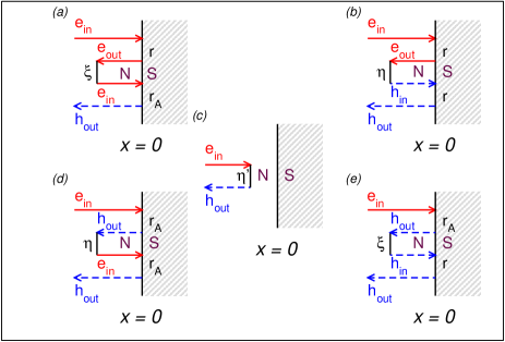
Figure 2: The processes that contribute to the amplitude for an incoming electron to transform to an outgoing hole. Note that all the processes shown here are to first order in the interaction parameters since they only involve a single scattering from a Friedel oscillation or the pair potential. Process $(c)$ involves scattering from a pair potential before the electron reaches the junction. The remaining processes involve two reflections from the junction and a scattering from the Friedel oscillation or the pair potential. In the diagrams, $\xi=\frac{1}{2}\,\alpha\,r^{\star}\,{\ln(kd)}$, $\eta=-\,\frac{1}{2}\,\alpha^{\prime}\,r_{A}^{\star}\,\ln(kd)$ and $\eta^{\prime}=\frac{1}{2}\,\alpha^{\prime}\,r_{A}\,\ln(kd)$.

Adding all the contributions, we obtain the change in the AR amplitude $r_{A}$ that takes an incoming electron to an outgoing hole given by

$$\delta r_{A} = {\displaystyle\frac{\alpha^{\prime}}{2}}\big{[}\,r_{A}\,-\,r_{A}^{\star}\left(r^{2}+r_{A}^{2}\right)\,\big{]}\,\ln(kd)$$ (20)

$$+~{}\alpha\,|r|^{2}\,r_{A}\,\ln(kd)$$

in agreement with Ref. jap2, . For an incoming electron reflected back as an electron, we find the small correction in the amplitude $\delta r$ given by yue ; lal

$${{\delta r}} = {{-\alpha^{\prime}\,|r_{A}|^{2}\,r\,\ln(kd)}}$$ (21)

$${{+~{}\frac{\alpha}{2}\,\left[\,r_{A}^{2}\,r^{\star}\,-\,r\left(1\,-\,|r|^{2}\right)\,\right]\ln(kd)}}$$

We replace $-\ln(kd)$ by $dl$ using the “poor man’s scaling” approach anderson to obtain the RG equation for $r_{A}$ as

$$\frac{dr_{A}}{dl} = -\,\frac{\alpha^{\prime}}{2}\left[r_{A}\,-\,r_{A}^{\star}\left(r^{2}\,+\,r_{A}^{2}\right)\right]\,-\,\alpha\,|r|^{2}r_{A}$$ (22)

Using the unitarity of the $S$-matrix ($|\,r_{A}\,|^{2}+|\,r^{2}\,|=1$ and $r_{A}^{\star}r+r_{A}r^{\star}=0$), we can simplify the RHS of the above equation to obtain

$$\frac{dr_{A}}{dl} = -\,\left(\,\alpha\,+\,\alpha^{\prime}\,\right)\,r_{A}\left(\,1-|r_{A}|^{2}\,\right)$$ (23)

Note that the combination $\alpha\,+\,\alpha^{\prime}=(2\,g_{2}-g_{1})/2\pi\hbar v_{F}$ which appears in the RG equation does not flow under RG. This can be seen from Eqs. 3 and LABEL:intrg2 which shows that $(2\,g_{2}-g_{1})/2\pi\hbar v_{F}=(2V(0)-V(2k_{F}))/2\pi\hbar v_{F}$. This means that $r$ and $r_{A}$ either monotonically increase or decrease as a power law depending on the sign of $\alpha\,+\,\alpha^{\prime}$. From Eq. 23, we also observe that $|r_{A}|=0$ and $|r_{A}|=1$ correspond to the insulating and the Andreev fixed points of the NS junction respectively. One can easily see from the RG equations that $|r_{A}|=0$ is a stable fixed point and $|r_{A}|=1$ is an unstable fixed point.

IV.2 NSN Junction

In this subsection, we shall consider an NSN junction. Here in addition to the two reflection channels, we also have two channels for transmission - the direct transmission of an electron to an electron through CT process and the transmission of an electron to a hole via CAR. These processes are depicted in Fig. 3. The $S$-matrix at the junction is $8\times 8$ in this case as given in Eq. 6.

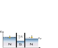
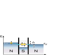
Figure 3: Electron CT with bare amplitude $t$ is shown in the left plot and CAR with bare amplitude $t_{A}$ is shown in the right plot.

The number of processes that contribute in this case is thirty four, since we also need to include terms that transmit electrons or holes through the junction. For instance, for the renormalization of the AR term, besides the terms corresponding to the NS junction, we also have to include processes in which the electron is incident from wire $1$, goes through the junction to wire $2$, Andreev reflects from the pair potential on wire $2$ and then comes back through the junction, as shown pictorially in Fig. 4(c).

Collecting all the nine processes that contribute to first order in $\alpha$ and $\alpha^{\prime}$ to the reflection amplitude, we find that

$${\displaystyle\frac{dr}{dl}} = -\bigg{[}{\displaystyle\frac{\alpha}{2}}\,\left[(t^{2}\,+\,r_{A}^{2}\,+\,t_{A}^{2})\,r^{\star}\,-\,r(1-|r|^{2})\right]$$ (24)

$$- \alpha^{\prime}\,(r\,|r_{A}|^{2}\,+\,r_{A}^{\star}\,t_{A}\,t)\bigg{]}$$

Similarly, adding up the contributions from the nine processes that contribute to $r_{A}$, we find that

$${\displaystyle\frac{dr_{A}}{dl}} = -\bigg{[}\alpha(|r|^{2}\,r_{A}\,+\,t\,t_{A}\,r^{\star})$$ (25)

$$+ {\displaystyle\frac{\alpha^{\prime}}{2}}(r_{A}\,-\,(r^{2}\,+\,r_{A}^{2}\,+\,t^{2}\,+\,t_{A}^{2})\,r_{A}^{\star})\bigg{]}$$

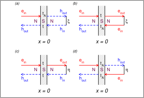
Figure 4: The extra processes that contribute to the amplitude for an incoming electron to transform to an outgoing hole on the same wire, due to the second wire. Processes (a) and (b) are transmitted to the second wire and reflected by the Friedel oscillation whereas (c) and (d) are transmitted to the second wire and reflected by the pair potential.

Moreover, here besides the reflection parameters, we also need to compute the renormalizations of the transmissions to first order in $\alpha$ and $\alpha^{\prime}$. The RG equations for $t$ and $t_{A}$ are also obtained by considering all possible processes that ultimately have one incoming electron and one outgoing electron (for $t$) and one incoming electron and one outgoing hole (for $t_{A}$) and are either reflected once from the Friedel potential or the pair potential. They are found to be

$${\displaystyle\frac{dt}{dl}} = -\,\bigg{[}\alpha\,(|r|^{2}\,t\,+\,r^{\star}\,r_{A}\,t_{A})$$ (26)

$$- \alpha^{\prime}\,(|r_{A}|^{2}\,t\,+\,r\,r_{A}^{\star}\,t_{A})\bigg{]}$$

$${\displaystyle\frac{dt_{A}}{dl}} = -\,\bigg{[}\alpha(r^{\star}\,r_{A}\,t\,+\,|r|^{2}\,t_{A})$$ (27)

$$- \alpha^{\prime}\,(r\,t\,r_{A}^{\star}\,+\,|r_{A}|^{2}\,t_{A})\bigg{]}$$

Just as was done for the normal junction (Eq.5), we can express the RG equations for the superconducting junction in a compact matrix form lal ,

$$\frac{dS}{dl}={\tilde{F}}-S{\tilde{F}}^{\dagger}S$$ (28)

where the matrix $S$ is given in Eq.6 and $\tilde{F}$ depends on the interaction parameters $\alpha=(g_{2}-2g_{1})/2\pi\hbar v_{F}$ and $\alpha^{\prime}=(g_{1}+g_{2})/2\pi\hbar v_{F}$. $\tilde{F}$ is non-diagonal matrix (unlike the case in Ref. lal, ) and is given by

$${\tilde{F}}~{}=~{}\begin{vmatrix}~{}\frac{\alpha r}{2}&0&\frac{-\alpha^{\prime}r_{A}}{2}&0~{}\\ ~{}0&\frac{\alpha r}{2}&0&\frac{-\alpha^{\prime}r_{A}}{2}~{}\\ ~{}\frac{-\alpha^{\prime}r_{A}}{2}&0&\frac{\alpha r}{2}&0~{}\\ ~{}0&\frac{-\alpha^{\prime}r_{A}}{2}&0&\frac{\alpha r}{2}~{}\\ \end{vmatrix}~{}.$$ (29)

It is easy to check that all the RG equations are reproduced from the matrix equation. The matrix form also makes the generalization to $N$ wires case notationally simple and makes the search for various fixed point much easier. This will be discussed in the last section. But note that these equations have to be augmented by Eqs. 3 and LABEL:intrg2 to get the full set of RG equations.

Let us now look at some of the fixed points of the $S$-matrix. Clearly, the fixed points occur when $F-SF^{\dagger}S=0$ or when $FS^{\dagger}$ is hermitian. There are several possibilities and we list below some of them.

1. Case I: Any one of the four parameters is non-zero
   (a) $t=1$, $r=r_{A}=t_{A}=0$, fully transmitting fixed point (TFP)
   (b) $r=1$, $r_{A}=t_{A}=t=0$ fully reflecting fixed point (RFP)
   (c) $r_{A}=1$, $r=t=t_{A}=0$, fully Andreev reflecting fixed point (AFP)
   (d) $t_{A}=1$, $r=t=r_{A}=0$, fully crossed Andreev reflecting fixed point. (CAFP)

2. Case II: Any two are non-zero
   When both $r$ and $r_{A}$ are zero, the RHS of the RG equations identically vanishes as both the Friedel oscillation amplitude as well as the pair potential amplitude in the wire become zero. Hence any value of $t$ and $t_{A}$ remains unrenormalized under RG.

3. Case III: Any three of them are non-zero
   We did not find any fixed point of this type.

4. Case IV: All four of them are non-zero
   Here, we get a fixed point when $r_{1}=r_{2}=t=t_{A}=1/2$ and $r_{A1}=r_{A2}=-1/2$. This is the most symmetric $S$-matrix possible for the NSN case. Since it is a symmetry-dictated fixed point with intermediate transmission and reflection, we shall refer to it as symmetric fixed point (SFP).

We will study the RG flows near some of these fixed points in the next section.

IV.3 FS, FSF and FSN Junctions

We can also consider junctions where one or more of the wires are spin-polarised, with Fermi distributions for the spin up and down electrons being different. As long as at least one of the wires is ferromagnetic, the spin up-spin down symmetry of the system is broken. This means that we can no longer impose $S_{\uparrow}=S_{\downarrow}$ on the $S$-matrix parametrising the scattering as we had in Eq.6. We now need to choose an $S$-matrix with indices $\uparrow$ and $\downarrow$ denoting the spin. For the FSN case (and the FSF case where the ferromagnets on the two sides are not identically polarized) the wire index symmetry is also broken. Hence, the $S$-matrix chosen must also break the wire-index symmetry. Note that for the ferromagnetic wire, the amplitude to destroy a spin $s$ electron and create a spin $s$ hole cannot be non-zero, even in the proximity of the superconductor. The Boguliobov amplitudes $\langle~{}d_{ik-s}^{\dagger}b_{iks}^{\dagger}~{}\rangle$ and $\langle~{}b_{iks}d_{ik-s}~{}\rangle$ decay exponentially fast (with a length scale set by the ferro$-$anti-ferro gap) in the ferromagnetic wire. So, in our $S$-matrix, $r_{A}$ is zero and there is no pair potential due to the proximity effect in ferromagnetic wire. Also as mentioned earlier, we must keep in mind that the influence of the ferromagnet on the spectrum of the superconductor has to be negligibly small. This will be true only if the superconductor is large enough. Hence, for such junctions, the renormalization of the $S$-matrix is only due to the Friedel oscillations. Also note that in these wires, since the bulk does not have both the spin species, $g_{1}$ and $g_{2}$ do not get renormalized. All the cases mentioned above will therefore involve the full $4N\times 4N$ $S$-matrix since there is no reduction in number of independent elements of the $S$-matrix which can occur when symmetries are imposed.

IV.4 Three$-$Wire$-$Junction $-$ A Beam Splitter

In this subsection, we consider the standard beam splitter geometry comprising of a superconductor at the junction of three quantum wires. In this case, we show that there is a fixed point that is analogous to the Andreev fixed point of the NS junction. The $S$-matrix representing this fixed point is symmetric under all possible permutations of the three wires and allows for the maximum Andreev transmission (in all channels simultaneously within unitarity constraints). The $S$-matrix is given by $r_{A}=-1/3$ and $t_{A}=t_{A}^{\prime}=2/3$ with $r=t=t^{\prime}=0$. We refer to this fixed point as the Andreev$-$Griffith’s fixed point (AGFP) .

For an analytic treatment of this case, we will consider a simplified situation where there is a complete symmetry between two of the wires, say $1$ and $2$, and the $S$-matrix is real. In addition, the elements of the $S$-matrix corresponding to transmission or reflection of an incident electron (hole) to a reflected or transmitted electron (hole) are set to zero so that only Andreev processes participating in transport. Then the $S$-matrix is given by

$$S=\begin{vmatrix}~{}0&0&0&r_{A}&t_{A}&t_{A}^{\prime}~{}\\ ~{}0&0&0&t_{A}&r_{A}&t_{A}^{\prime}~{}\\ ~{}0&0&0&t_{A}^{\prime}&t_{A}^{\prime}&r_{A}^{\prime}~{}\\ ~{}r_{A}&t_{A}&t_{A}^{\prime}&0&0&0~{}\\ ~{}t_{A}&r_{A}&t_{A}^{\prime}&0&0&0~{}\\ ~{}t_{A}^{\prime}&t_{A}^{\prime}&r_{A}^{\prime}&0&0&0~{}\\ \end{vmatrix}$$ (30)

Here, $r_{A}$ and $t_{A}$ and $t^{\prime}_{A}$ are real parameters which satisfy das

$$t_{A} = 1+r_{A}~{},$$

$$r^{\prime}_{A} = -1-2r_{A}~{},$$

$$t^{\prime}_{A} = \sqrt{(-2r_{A})(1+r_{A})}~{},$$

$${\mathrm{and}}\quad-1 \leq r_{A}\leq 0$$ (31)

by unitarity. Using Eq. 31, the simplified RG equation for the single parameter $r_{A}$ is given by

$${\displaystyle\frac{dr_{A}}{dl}}=\alpha^{\prime}~{}\left[r_{A}(1+r_{A})(1+3r_{A})\right]$$ (32)

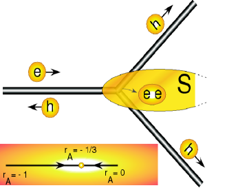
Figure 5: Schematic representation of the situation where a three$-$wire$-$junction is hooked to the stable fixed point, AGFP. An incident electron in one wire is either reflected back as a hole in the same wire or is transmitted as a hole in another wire along with the addition of the two electrons into the superconductor forming a Cooper pair. The direction of RG flow from two unstable fixed points to the stable fixed point (AGFP) is also depicted on the bottom left side of the diagram.

So, within the real parametrization we have two unstable fixed points, given by $r_{A}=0$ and $r_{A}=-1$ and a stable fixed point given by $r_{A}=-1/3$. The $r_{A}=0$ fixed point corresponds to a situation where there is perfect CAR between wires $1$ and $2$ and wire $3$ gets cut off from the remaining two wires (labelled by $1$ and $2$) and is in the perfect AR limit with the superconductor. The $r_{A}=-1$ fixed point corresponds to a situation where all the three wires are disconnected from each other and are in perfect AR limit individually with the superconductor. The third fixed point given by $r_{A}=-1/3$ corresponds to a perfect Andreev limit of the three wire junction where an incident electron is either Andreev-reflected into the same wire as a hole or is transmitted as a hole via CAR into another wire. This is essentially the AGFP. It is very interesting to note that the original Griffith’s fixed point was a repulsive fixed point lal ; das whereas the AGFP is an attractive fixed point. This can be understood as follows. Here, there is no scattering from the Friedel oscillations as the junction is assumed to be reflection-less, whereas there exists a proximity induced pair potential, which induces an effective attractive interaction between the electrons. Hence, the physics is very similar to the well-known Luttinger Liquid physics, which says that for attractive interaction between the electrons, back-scattering is an irrelevant operator. Hence the stable fixed point here will be the one which will have maximal transmission between the wires. So, it is not surprising that the AGFP turns out to be a stable fixed point. Thus, for a reflection-less junction, we have found a stable fixed point with intermediate transmission and reflection.

V Results

In this section, we will consider various physical cases and see what the RG flows mean for the conductances in each case.

V.1 NS Junction

First, we give the results for the NS junction, just to contrast with the results of the NSN junction. Here, we have only two parameters, $r$ and $r_{A}$. The conductance occurs only due to the AR amplitude, $r_{A}$ which obeys the RG equation given by Eq. 20. As mentioned already, there is no flow of the particular linear combination of the interaction parameters $2g_{2}-g_{1}$ that occurs in the equation and the RG flow of the conductance is therefore monotonic. The conductance as a function of the length scale for different interaction parameters $V(0)$ and $V(2k_{F})$ is plotted in Fig. 6. $L$ here simply denotes the length at which the RG is cut-off. So if we take very long wires $L_{W}\gg L_{T}$, then the cut-off is set by the temperature, and the plot shows the variation of the conductance as a function of $L_{T}$ starting from the high temperature limit, which here is the superconducting gap $\Delta$. We observe that as we lower the temperature, the Andreev conductance decreases monotonically. Also it was established in Ref.jap3, that the power law scaling of conductance ($~{}|r_{A}|^{2}$) calculated from WIRG and bosonization were found to be in agreement with each other for the limiting cases of $|r_{A}|^{2}\cong 1$ and $~{}|r_{A}|^{2}\cong 0$ ( which are the only limits where bosonization results are valid) provided effects due to electron-electron induced back-scattering in the wires is neglected.

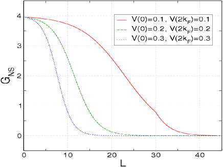
Figure 6: Conductance of the NS junction is plotted in units of $e^{2}/h$ as a function of the dimensionless parameter $l$ where $l=ln(L/d)$ and $L$ is either $L_{T}=\hbar v_{F}/k_{B}T$ at zero bias or $L_{V}=\hbar v_{F}/eV$ at zero temperature and $d$ is the short distance cut-off for the RG flow. The three curves correspond to three different values of $V(0)$ and $V(2k_{F})$.

V.2 Ballistic NSN Junction

In this subsection, we consider the case of a reflection-less ballistic junction between the superconductor and the two wires, i.e. $r=0$. This implies that the renormalization of the $S$-matrix due to the Friedel oscillations is absent. The only renormalization is due to reflections from the proximity effect induced pair potential. Let us now consider various interesting cases:

1. (a) $r=0,r_{A}=0,t\neq 0,t_{A}\neq 0$. In this case, since we have both $r=0$ and $r_{A}=0$, there is no RG flow of the transmission and the conductance is frozen at the value that it had for the bare $S$-matrix. The most interesting situation in this case arises when $t=t_{A}$. For this case, the probability for an incident electron in one wire, to transmit in the other wire as an electron due to $t$ or as hole due to $t_{A}$ is equal, leading to perfect cancellation of charge current.

2. (b) $r=0,t=0,r_{A}\neq 0,t_{A}\neq 0$. For this case, one can easily check from the RG equations (Eqs. 24-27) that if we start our RG flow with the given parameters at high energies, then the value of $r,t$ remain stuck to the value zero under the RG flow. Hence, in this case the two parameter subspace $r_{A}\neq 0,t_{A}\neq 0$ remains secluded under the RG flow. The RG equation for $t_{A}$ is given by

   $${\displaystyle\frac{dt_{A}}{dl}} = \alpha^{\prime}\,t_{A}\,(1-|t_{A}|^{2})$$ (33)

   The above equation can be integrated to obtain an expression for CAR probability ($T_{A}=|t_{A}|^{2}$),

   $$T_{A}(L)=\frac{T_{A}^{0}\left[[1+2\alpha_{1}\ln(\frac{L}{d})]^{\frac{3}{2}}(\frac{d}{L})^{-(2\alpha_{2}-\alpha_{1})}\right]}{R_{A}^{0}+T_{A}^{0}\left[[1+2\alpha_{1}\ln(\frac{L}{d})]^{\frac{3}{2}}(\frac{d}{L})^{-(2\alpha_{2}-\alpha_{1})}\right]}$$ (34)

   $T_{A}^{0}$ and $R_{A}^{0}$ are the CAR and AR probabilities at the short distance cut-off, $L=d$. We notice that the RG equation and its solution are very similar to that for the single scatterer problem matveev apart from a sign difference on the RHS of the equation and the dependance of the interaction parameter $\alpha^{\prime}$ on $g_{1}$ and $g_{2}$. This implies that even if we start with a small crossed Andreev transmission across the junction, the RG flow will take us towards the limit of perfect transmission. This is in sharp contrast to the normal transmission across a single scatterer. For the single barrier problem, the equation for the RG flow of $t$ was by

   $${\displaystyle\frac{dt}{dl}} = -\alpha\,t\,(1-|t|^{2}).$$ (35)

   Hence, $t=0$ was the stable fixed point. But if the electron-electron interactions had been attractive, then the sign on the RHS would have been positive and $t=1$ would have been the stable fixed point. Thus, the RG flow of $t_{A}$ for the case when $r_{A}\neq 0,t=r=0$, and repulsive interactions, is very similar to the RG flow for $t$ when $r\neq 0,t_{A}=r_{A}=0$ but with attractive interactions. In both cases transmission is relevant and $t=1$ and $t_{A}=1$ are the stable fixed points. On the other hand the RG flow of $t_{A}$ for the case of $r_{A}\neq 0,t=0,r=0$ and attractive electron-electron interaction ($V(0),V(2k_{F})<0$) in the wire is very similar to the RG flow for $t$ for the case $r\neq 0,r_{A}=0,t_{A}=0$ and repulsive electron-electron interaction ($V(0),V(2k_{F})>0$). In both cases transmission is irrelevant and $t=0$ and $t_{A}=0$ are the stable fixed points. At an intuitive level, one can perhaps say that even if we start with repulsive inter-electron interactions, the proximity-induced pair potential leads to a net attractive interaction between the electrons, which is responsible for the counter-intuitive RG flow.

   Also notice that while solving the above RG equation for $t_{A}$, we have to take into account the RG flow of the interaction parameter ($\alpha^{\prime}$) itself. This will lead to non-power law (non Luttinger) behavior for the conductance close to $|t_{A}|\,\simeq\,0$ or $|t_{A}|\,\simeq\,1$. It is worth pointing out that the non-power law part appearing in Eq. 34 is identical to Ref. matveev, , even though the interaction parameter for their case was proportional to $g_{2}-2g_{1}$ and for our case it is $g_{2}+g_{1}$. But of course this will not lead to any non-monotonic behavior as $\alpha^{\prime}$ can not change sign under RG flow. So the stable fixed point for this case is the CAFP.

3. (c) $r=0,t_{A}=0,r_{A}\neq 0,t\neq 0$. This case is identical to the case (b) discussed above except for the fact that we have to replace $t_{A}$ in the previous case by $t$. In this case also the two parameter subspace $r_{A}\neq 0,t\neq 0$ remains secluded under RG flow. The RG equation for $t$ is given by

   $${\displaystyle\frac{dt}{dl}} = \alpha^{\prime}t(1-|t|^{2})$$ (36)

   Here also, $t=1$ remains the stable fixed point and $t=0$ is the unstable fixed point.

4. (d) $r=0,t\neq 0,r_{A}\neq 0,t_{A}\neq 0$. In this case if we start from a symmetric situation, i.e. $t=t_{A}$, we can see from the RG equations in Eqs. 26 and 27 that both $t$ and $t_{A}$ have identical RG flows. So, the sub-gap conductance $G=G_{CA}-G_{CT}$ vanishes identically and remains zero through out the RG flow. Hence this $S$-matrix can facilitate production of pure SC drsahaepl if we inject spin polarized electrons from one of the leads as the charge current gets completely filtered out at the junction.

V.3 Ballistic FSF Junction

Here, we consider the case where both the wires are spin polarized. In this case we have two interesting possibilities, i.e.  either both the wires have aligned spin polarization or they have them anti-aligned. In either case the Andreev reflection amplitude is zero on each wire due to reasons explained earlier.

1. (a) When the two wires have their spins aligned, $t\neq 0$, but $t_{A}=0$ because for CAR to happen we need up(down) spin polarization in one wire and down(up) spin polarization on the other wire which is not possible in this case.

2. (b) When the two wires have their spins anti-aligned, $t=0$, but $t_{A}\neq 0$ because the up(down) electron from one wire can not tunnel without flipping its spin into the other wire. As there is no mechanism for flipping the spin of the electron at the junction, such processes are not allowed.

Hence these two cases can help in separating out and measuring amplitudes of the direct tunneling process and the CAR process experimentally beckmann . Both these are examples of case II, since they have both $r=0$ and $r_{A}=0$. In this case, neither $t$ nor $t_{A}$ change under RG flow and hence conductance is not influenced by electron-electron interaction at all.

V.4 Non-ballistic NSN Junction

V.4.1 Without AR on individual wires

Here we consider an NSN junction with finite reflection in each wire and no AR in the individual wires. So the renormalization of the $S$-matrix is purely due to Friedel oscillations and there are no contributions coming from scattering due to the pair potential. Below we discuss two cases :

1. (a) $r_{A}=0,t=0,r\neq 0,t_{A}\neq 0$. This is an example of case II mentioned in Subsection. IV.2. The RG equations (Eqs. 24-27) predict that $r_{A},t$ will remain zero under the RG flow and $r,t_{A}$ form a secluded sub-space. The RG equation for this case is given by

   $${\displaystyle\frac{dt_{A}}{dl}} = -\,\alpha\,t_{A}(1-|t_{A}|^{2})$$ (37)

   Note the change in sign on the RHS with respect to the RG equation for $t_{A}$ (Eq. 33) for the ballistic case. This change in sign represents the fact that the ballistic case effectively represents a situation corresponding to attractive electron-electron interaction while this case corresponds to a purely repulsive electron-electron interaction.

   Fig. 7 shows the behavior of conductance ($G_{CA}$) for this case. The conductance in the main graph shows a non-monotonic behavior.

   

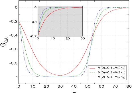
   Figure 7: Conductance $G_{CA}$ of the NSN junction is plotted (when the two leads have anti-parallel spins) in units of $e^{2}/h$ as a function of the dimensionless parameter $l$ where $l=ln(L/d)$ and $L$ is either $L_{T}=\hbar v_{F}/k_{B}T$ at zero bias or $L_{V}=\hbar v_{F}/eV$ at zero temperature and $d$ is the short distance cut-off for the RG flow. The three curves correspond to three different values of $V(0)$ and $V(2k_{F})$. The inset shows the behavior of the same conductance for fixed values of $\alpha$.

   To contrast, we also show in the inset, the behavior when the renormalization of $\alpha$ in not taken into account. Thus, it is apparent from the plot that the non-monotonicity is coming solely from the RG evolution of $\alpha$. The inset and the main graph, both start from the same value of $t_{A}$. Even though this case is theoretically interesting to explore, its experimental realization may not be viable. This is because of the following reasons. Here we have $r_{A}=0$ on both wires, which can only happen if the wires are ferromagnetic. However, we also know that if the wires are ferromagnetic, there is no scaling of $\alpha$ parameter and hence there will be no interesting non-monotonic trend in the conductance. So it is hard to find a physical situation where $r_{A}=0$ and at the same time, there is renormalization of the interaction parameter $\alpha$. Lastly note that the conductance $G_{CA}$ is negative. The process responsible for the conductance, (i.e. CAR), converts an incoming electron to an outgoing hole or vice-versa, resulting in the negative sign.

2. (b) $r_{A}=0,t_{A}=0,r\neq 0,t\neq 0$. This case is identical to the previous case with the replacement of $t_{A}$ by $t$. Fig. 8 shows the the CT conductance $G_{CT}$ as a function of the length scale. It shows a similar non-monotonic behavior with positive values for the conductance. The inset shows the behavior of $G_{CT}$ when the renormalization of $\alpha$ in not taken into account.

   

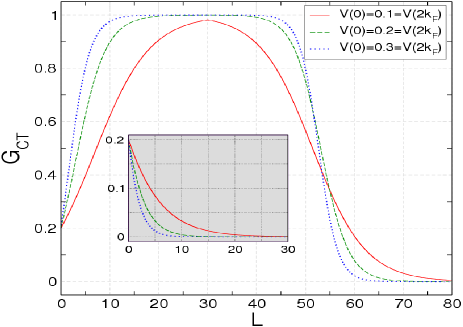
   Figure 8: Conductance $G_{CT}$ of the NSN junction (when the two leads have parallel spins) in units of $e^{2}/h$ as a function of the dimensionless parameter $l$ where $l=ln(L/d)$ and $L$ is either $L_{T}=\hbar v_{F}/k_{B}T$ at zero bias or $L_{V}=\hbar v_{F}/eV$ at zero temperature and $d$ is the short distance cut-off for the RG flow. The three curves correspond to three different values of $V(0)$ and $V(2k_{F})$. The inset shows the behavior of the same conductance for fixed values of $\alpha$.

   V.4.2 With AR on individual wires

3. (a) $r_{A}\neq 0,t_{A}\neq 0,r\neq 0,t\neq 0$. This is the most interesting case, where both $r$ and $r_{A}$ are non-zero, and we get an interplay of the effects due to scattering from Friedel oscillations and from proximity induced pair potential. Here, all the four parameters are non-zero and flow under RG, as do the interaction parameters $\alpha$ and $\alpha^{\prime}$. An example where the system starts in the vicinity of the unstable fixed point SFP (as mentioned in Case IV in the Subsection. IV.2) is shown in Fig. 9. The NSN conductance here is defined as $G_{NSN}=G_{CA}-G_{CT}$. Here also we observe a strong non-monotonicity in the conductance which comes about due to interplay of the electron and the hole channels, which contribute to the conductance with opposite signs, coupled with the effects from the RG flow of the interaction parameters.

V.5 Non-ballistic FSN Junction

In this case, for the ferromagnetic wire $r_{A}=0$, but for the normal wire $r_{A}$ has a finite value. As explained earlier, the interaction parameters $\alpha$ and $\alpha^{\prime}$ on the ferromagnetic side do not renormalize, whereas they do on the normal side. Hence, even if we start from a situation where the interaction parameter $\alpha$ and $\alpha^{\prime}$ are symmetric for the two wires, RG flow will always give rise to an asymmetry in the interaction strength. Therefore, it becomes a very interesting case to study theoretically. The $S$-matrix for this case has neither spin up-spin down symmetry, nor the wire index (left-right for two wires) symmetry. Only the particle-hole symmetry can be retained while parameterizing the $S$-matrix. This case gets very complicated to study theoretically because the minimum number of independent complex-valued parameters that are required to parameterize the $S$-matrix is nine as opposed to four in the NSN case. These are given by $r_{\uparrow\uparrow}^{11},~{}r_{\uparrow\uparrow}^{22},~{}r_{\downarrow\downarrow}^{22},~{}t_{A\uparrow\uparrow}^{12},~{}t_{A\downarrow\downarrow}^{21},~{}r_{A\uparrow\uparrow}^{22},~{}r_{A\downarrow\downarrow}^{22},~{}t_{\uparrow\uparrow}^{12},~{}{\mathrm{and}}~{}t_{\uparrow\uparrow}^{21}$. Here, $1$($2$) is the wire index for the ferromagnetic (normal) wire while, $\uparrow$ and $\downarrow$ are the respective spin polarization indices for the electron.

So, the minimal $S$-matrix representing the FSN junction is given by

$$S~{}=~{}\begin{vmatrix}~{}r&t&0&0&t_{A}&0~{}\\ ~{}t^{\prime}&r^{\prime}&0&0&r_{A}&0~{}\\ ~{}0&0&r^{\prime\prime}&t_{A}^{\prime}&0&r_{A}^{\prime}~{}\\ ~{}0&0&t_{A}&r&0&t~{}\\ ~{}t_{A}^{\prime}&r_{A}^{\prime}&0&0&r^{\prime\prime}&0~{}\\ ~{}0&0&r_{A}&t^{\prime}&0&r^{\prime}~{}\\ \end{vmatrix}$$ (38)

The RG equations for the nine independent parameters are given in Appendix A. We write down a representative $S$-matrix which satisfies all the constraints of the FSN junction and unitarity, and study its RG flow numerically by solving the nine coupled differential equations. The modulus of the $S$-matrix elements are given by $|r_{\uparrow\uparrow}^{11}|=|r_{\uparrow\uparrow}^{22}|=|r_{\downarrow\downarrow}^{22}|=|t_{A\uparrow\uparrow}^{12}|=|t_{A\downarrow\downarrow}^{21}|=|r_{A\uparrow\uparrow}^{22}|=|r_{A\downarrow\downarrow}^{22}|=|t_{\uparrow\uparrow}^{12}|=\lvert t_{\uparrow\uparrow}^{21}\rvert=1/\sqrt{3}$ and the corresponding phases associated with each of these amplitudes are $\pi/3,\pi,0,-\pi/3,0,\pi/3,0,\pi,-\pi/3$ respectively. Here also we observe a non-monotonic behavior of conductance, $G_{FSN}$ as a function of $l$ as shown in Fig. 9.

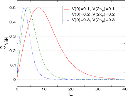
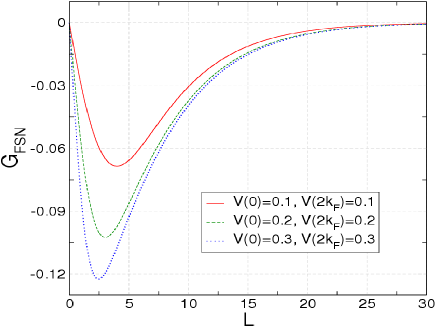
Figure 9: Left: Conductance of the NSN junction $G_{NSN}=|t_{A}|^{2}-|t|^{2}$ is plotted in units of $2e^{2}/h$ as a function of the dimensionless parameter $l$ where $l=ln(L/d)$ and $L$ is either $L_{T}=\hbar v_{F}/k_{B}T$ at zero bias or $L_{V}=\hbar v_{F}/eV$ at zero temperature and $d$ is the short distance cut-off for the RG flow. The three curves correspond to three different values of $V(0)$ and $V(2k_{F})$. Right: Charge conductance $G_{FSN}=|t_{A}|^{2}-|t|^{2}$ is plotted for FSN case as a function of the dimensionless parameter $l$ where $l=ln(L/d)$ and $L$ is either $L_{T}=\hbar v_{F}/k_{B}T$ at zero bias or $L_{V}=\hbar v_{F}/eV$ at zero temperature in units of $e^{2}/h$ and $d$ is the short distance cut-off for the RG flow. The three curves correspond to three different values of $V(0)$ and $V(2k_{F})$.

V.6 Non-ballistic FSF junction

Here, we will consider the case where both the wires are spin polarized. This case is similar to the ballistic case. Since here $r\neq 0$ and $r_{A}=0$, we will have the usual Friedel oscillations and the conductance will go to zero as a power law. Here again we have two instructive cases:

1. (a) When the two wires connected to the superconductor have their spin polarization aligned, i.e. $t\neq 0$, but $t_{A}=0$ and

2. (b) When the two wires have their spin polarization anti-aligned, $i.e.$, $t=0$ but $t_{A}\neq 0$.

Both these are examples of case II of Subsection. IV.2. Either $t$ or $t_{A}$ need to be zero in the two cases mentioned above. Hence the parameters which are zero will remain zero under RG , while the non-zero parameters will flow according to Eqs. 26 and 27 respectively. The conductances are the same as in the NSN case except that the interaction parameters cannot flow now. This has already been plotted in the insets in Figs. 7 and 8. Since the electrons are now effectively spin-less, $\alpha$ and $\alpha^{\prime}$ do not flow, and we get a monotonic fall-off of the conductance in both the cases.
The results of this section are summarized in the table below.

$t$	$t_{A}$	$r_{A}$	$r$	Stability	Intermediate fixed point	Relevant physics
0	0	0	1	Stable	$\times$	RFP
0	0	1	0	Unstable	$\times$	AFP
0	1	0	0	Unstable	$\times$	CAFP
1	0	0	0	Unstable	$\times$	TFP
1/2	1/2	-1/2	1/2	Unstable	$\surd$	SFP, Non-monotonic charge current
$e^{i\phi_{1}}\sin\theta$	$e^{i\phi_{2}}\cos\theta$	0	0	Marginal	$-$	Pure spin current when $t=t_{A}$

VI Generalization to the case of three wires

In this section, we consider the case of three wires connected to a superconductor. We assume that all the wires are connected within the phase coherence length of the superconductor. Hence, CAR can occur by pairing the incident electron with an electron from any of the other wires and emitting a hole in that wire. The conductance matrix can hence be extended for three wires as

$$\begin{vmatrix}~{}I_{1}~{}\\ ~{}I_{2}~{}\\ ~{}I_{3}~{}\\ \end{vmatrix}=\begin{vmatrix}~{}G_{r\,11}&G_{t\,12}&G_{t\,13}~{}\\ ~{}G_{t\,12}&G_{r\,22}&G_{t\,23}~{}\\ ~{}G_{t\,13}&G_{t\,23}&G_{r\,33}~{}\\ \end{vmatrix}\begin{vmatrix}~{}V_{1}~{}\\ ~{}V_{2}~{}\\ ~{}V_{3}~{}\\ \end{vmatrix}$$ (39)

with $G_{r\,ij}=G_{{A\,ii}}+\sum_{j}(G_{{CA\,ij}}+G_{{CT\,ij}})$ and $G_{t\,ij}=G_{{CA\,ij}}-G_{{CT\,ij}}$ and the generalization to $N$ wires is obvious. Note that the conductances $G_{CA\,ij}=G_{CA\,ji}$ and $G_{CT\,ij}=G_{CT\,ji}$. The relations of the conductances to the reflections and transmissions is obvious, for e.g., $G_{A\,ii}\propto|r_{A\,ii}|^{2}$ as before while $G_{CT\,ij}\propto|t_{ij}|^{2}$ and $G_{CA\,ij}\propto|t_{A\,ij}|^{2}$. The RG equations for the three wire case can be written using the matrix equation as given in Eq. 6 except that the $S$ matrix is now $12\times 12$ dimensional. For a system with particle-hole, spin up-spin down and wire index symmetry, the $S$ matrix is given by,

$$S_{\uparrow}=S_{\downarrow}=\begin{vmatrix}~{}r&t&t^{\prime}&r_{A}&t_{A}&t_{A}^{\prime}~{}\\ ~{}t&r&t&t_{A}&r_{A}&t_{A}~{}\\ ~{}t^{\prime}&t&r&t_{A}^{\prime}&t_{A}&r_{A}~{}\\ ~{}r_{A}&t_{A}&t_{A}^{\prime}&r&t&t^{\prime}~{}\\ ~{}t_{A}&r_{A}&t_{A}&t&r&t~{}\\ ~{}t_{A}^{\prime}&t_{A}&r_{A}&t^{\prime}&t&r~{}\\ \end{vmatrix}$$ (40)

where we have chosen six independent parameters, with $t_{12}=t_{21}=t_{23}=t_{32}=t$ and $t_{13}=t_{31}=t^{\prime}$ and similarly for the CAR parameter $t_{A}$. The $F$ matrix now generalizes to

$$F=\begin{vmatrix}~{}\frac{\alpha r}{2}&0&0&\frac{-\alpha^{\prime}r_{A}}{2}&0&0~{}\\ ~{}0&\frac{\alpha r}{2}&0&0&\frac{-\alpha^{\prime}r_{A}}{2}&0~{}\\ ~{}0&0&\frac{\alpha r}{2}&0&0&\frac{-\alpha^{\prime}r_{A}}{2}~{}\\ ~{}\frac{-\alpha^{\prime}r_{A}}{2}&0&0&\frac{\alpha r}{2}&0&0~{}\\ ~{}0&\frac{-\alpha^{\prime}r_{A}}{2}&0&0&\frac{\alpha r}{2}&0~{}\\ ~{}0&0&\frac{-\alpha^{\prime}r_{A}}{2}&0&0&\frac{\alpha r}{2}~{}\\ \\ \end{vmatrix}$$ (41)

and the RG equations for the six independent parameters are given in Appendix B. There exists possibility of many more non-trivial fixed points in this case. For instance, the AGFP, as mentioned in Subsection. IV.4. As discussed in Subsection. IV.4, for the reflection-less case with symmetry between just two wires, this complicated $S$-matrix takes a very simple form, which can be dealt with analytically. Within the sub-space considered we found that the AGFP was a stable fixed point. In Fig. 10, we show the RG flow of $|t_{A}|^{2}$ from two different unstable fixed points to the stable AGFP.

The possibility of experimental detection of such a non-trivial fixed point with intermediate transmission and reflection is quite interesting. From this point of view, the AGFP is a very well-suited candidate as opposed to its counterpart, the Griffith’s fixed point lal ; das . For a normal junction of three 1–D QW, the $S$-matrix corresponding to $r=-1/3,t=2/3$ is a fixed point (Griffith’s fixed point), where $r$ and $t$ are the reflection and the transmission for a completely symmetric three wire junction. Even though it is an interesting fixed point, it turns out to be a repulsive one and hence the possibility of its experimental detection is very low. On the contrary, the AGFP, being an attractive fixed point, has a better possibility of be experimentally measured. The main point here is that even if we begin with an asymmetric junction, which is natural in a realistic experimental situation, the effect of interaction correlations are such that as we go down in temperature, the system will flow towards the symmetric junction. This can be inferred from the results shown in Fig. 10.

Figure 10: $|t_{A}|^{2}$ is plotted as a function of dimensionless parameter $l$ where $l=ln(L/d)$ and $L$ is either $L_{T}=\hbar v_{F}/k_{B}T$ at zero bias or $L_{V}=\hbar v_{F}/eV$ at zero temperature and $d$ is the short distance cut-off for the RG flow. The three curves correspond to three different values of $V(0)$ and $V(2k_{F})$. The set of curves in the top represent the RG flow of $|t_{A}|^{2}$ when the starting point is in the vicinity of $r_{A}=0$ fixed point while, the set of curves in the bottom half represent the RG flow of $|t_{A}|^{2}$ with starting point close to $r_{A}=-1$.

VII Summary and Discussions

To summarize, in this article we have studied transport through a superconducting junction of multiple 1–D interacting quantum wires in the spirit of the Landauer$-$Buttiker formulation. Using the WIRG approach we derived the RG equations for the effective $S$-matrix and obtained the various fixed point $S$-matrices representing the junction. In contrast to earlier RG studies, here, we had to include both particle and hole channels due to the proximity effect of the superconductor. Our study led to the finding of a novel fixed point with intermediate Andreev transmission and reflection even in the case of NSN junction (SFP). However, it turns out to be unstable fixed point and hence experimentally inaccessible. We found that transport across the superconducting junction depends on two independent interaction parameters, ($\alpha=(g_{2}\,-\,2g_{1})/2\pi\hbar v_{F}$) which is due to the usual correlations coming from Friedel oscillations for spin-full electrons and ($\alpha^{\prime}=(g_{2}\,+\,g_{1})/2\pi\hbar v_{F}$), which arises due to the scattering of electron into hole by the proximity induced pair potential in the QW. We computed the length scale (or temperature) dependance of the conductance taking into account interaction induced forward and back-scattering processes. We found a non-monotonic dependence of the conductance for the two-wire NSN superconducting junction in contract to the NS junction where the dependence is purely monotonic.

When more than two wires are attached to the superconductor, we found even more exotic fixed points like the AGFP which happens to be a stable fixed point for a reflection-less symmetric junction thus increasing its chances of being experimentally seen. But reflection is a relevant perturbation and asymmetry between different wires is likely to be a relevant parameter drsaha . Hence, the RG flow due to these perturbations will take the system to the RFPin the low energy limit. So, the experimental detection of AGFP fixed point will critically depend on how efficiently the conditions of reflectionlessness and symmetry can be maintained in the experimental setup. If the reflection and asymmetry are reduced to a large extent, then as we cool the system, the S-matrix at the junction is expected to flow very close to the AGFP fixed point. But ultimately, the RG flow will lead to enhancement of any initial small value of reflection and asymmetry and we will finally flow to the disconnected fixed point in the $T=0$ limit. Thus it would be an interesting experimental challenge to look for signature of the AGFP at intermediate temperatures.

Before we conclude, it is worth mentioning that the geometry studied in our paper is of direct interest for the production of non-local entangled electron pairs propagating in two different wires. These electron pairs are produced by Cooper pair breaking via crossed Andreev processes when the superconductor is biased with respect to the wires comprising the junction. One can ask if electron-electron interaction in the wires actually leads to enhancement of entangled electron pair production via the crossed Andreev processes. For example, we have observed that for the NSN junction with $r=0,t=0,r_{A}\neq 0,t_{A}\neq 0$, interaction can lead to enhancement of the crossed Andreev amplitude ($t_{A}$) under RG flow. This implies that for the case when the superconductor is biased with respect to the wires, inter-electron interactions enhance the production of non-local entangled pairs, for which the amplitude $t_{A}$ is relevant, as compared to local entangled pairs for which the amplitude $r_{A}$ would be relevant. This is consistent with the results of Recher and Lossrecher1 who also argued that it is energetically more favourable for the two entangled electrons of the Cooper pair to go into different wires, rather than the same wire. Finally the RG flow leads to a fixed point with $t_{A}=1$ where the system becomes a perfect entangler. A more general case would be when $r\neq 0,t\neq 0,r_{A}\neq 0,t_{A}\neq 0$. To study this case, one can start from the two wires SFPS-matrix and study the RG flow of $t_{A}$ for an S-matrix which is in the close vicinity of this fixed point. The result of this study is shown in Fig. 9. We show that starting from the short-distance cut-off $d$ the RG flow initially leads to enhancement of $t_{A}$ which will lead to an enhancement in the production of non-local entangled pairs. Hence, these studies establish the fact electron-electron interactions the wires can actually lead to an enhancement of non-local entangled electron pair production.

Appendix A

Here we give the RG equations for nine independent parameters in case of a FSN junction.

$${\displaystyle\frac{dr}{dl}} = \Big{[}{\displaystyle\frac{\beta}{2}}~{}r\left(1~{}-~{}|r|^{2}\right)-{\displaystyle\frac{\alpha}{2}}~{}\left(tr^{\prime\star}t^{\prime}~{}+~{}r^{\prime\prime\star}t_{A}t_{A}^{\prime}\right)~{}+~{}{\displaystyle\frac{\alpha\prime}{2}}~{}\left(tr_{A}^{\star}t_{A}^{\prime}~{}+~{}t_{A}r_{A}^{\prime\star}t^{\prime}\right)\Big{]}$$ (1)

$${\displaystyle\frac{dt}{dl}} = -\,\Big{[}{\displaystyle\frac{\beta}{2}}~{}|r|^{2}t~{}+~{}{\displaystyle\frac{\alpha}{2}}~{}\left(|r^{\prime}|^{2}t~{}+~{}t_{A}r^{\prime\prime\star}r_{A}^{\prime}\right)~{}-~{}{\displaystyle\frac{\alpha^{\prime}}{2}}~{}\left(r_{A}^{\star}r_{A}^{\prime}t~{}+~{}r^{\prime}r_{A}^{\prime\star}t_{A}\right)\Big{]}$$ (2)

$${\displaystyle\frac{dt_{A}}{dl}} = -\,\Big{[}{\displaystyle\frac{\beta}{2}}|r|^{2}t_{A}~{}+~{}{\displaystyle\frac{\alpha}{2}}~{}\left(|r^{\prime\prime}|^{2}t_{A}~{}+~{}tr^{\prime\star}r_{A}\right)~{}-~{}{\displaystyle\frac{\alpha^{\prime}}{2}}~{}\left(r_{A}^{\star}r^{\prime\prime}t~{}+~{}r_{A}r_{A}^{\prime\star}t_{A}\right)\Big{]}$$ (3)

$${\displaystyle\frac{dr^{\prime}}{dl}} = -\,\Big{[}{\displaystyle\frac{\beta}{2}}~{}r^{\star}tt^{\prime}+{\displaystyle\frac{\alpha}{2}}~{}[r^{\prime\prime\star}r_{A}r_{A}^{\prime}-r^{\prime}(1-|r^{\prime}|^{2})]~{}-~{}{\displaystyle\frac{\alpha^{\prime}}{2}}~{}r^{\prime}(r_{A}r_{A}^{\prime\star}+r_{A}^{\star}r_{A}^{\prime})\Big{]}$$ (4)

$${\displaystyle\frac{dr_{A}}{dl}} = -\,\Big{[}{\displaystyle\frac{\beta}{2}}~{}r^{\star}tt_{A}+{\displaystyle\frac{\alpha}{2}}~{}r_{A}(|r^{\prime}|^{2}~{}+~{}|r^{\prime\prime}|^{2})~{}+~{}{\displaystyle\frac{\alpha^{\prime}}{2}}~{}(r_{A}-r_{A}^{2}r_{A}^{\prime\star}-r_{A}^{\star}r^{\prime}r^{\prime\prime})\Big{]}$$ (5)

$${\displaystyle\frac{dt^{\prime}}{dl}} = -\,\Big{[}{\displaystyle\frac{\beta}{2}}~{}|r|^{2}t^{\prime}+\frac{\alpha}{2}~{}(|r^{\prime}|^{2}t^{\prime}+r_{A}r^{\prime\prime\star}t_{A}^{\prime})~{}-~{}{\displaystyle\frac{\alpha^{\prime}}{2}}~{}(r_{A}r_{A}^{\prime\star}t^{\prime}~{}+~{}r^{\prime}r_{A}^{\star}t_{A}^{\prime})\Big{]}$$ (6)

$${\displaystyle\frac{dr^{\prime\prime}}{dl}} = -\,\Big{[}{\displaystyle\frac{\beta}{2}}~{}r^{\star}t_{A}t_{A}^{\prime}~{}+~{}{\displaystyle\frac{\alpha}{2}}~{}[r^{\prime\star}r_{A}r_{A}^{\prime}-r^{\prime\prime}(1-|r^{\prime\prime}|^{2})]~{}-~{}{\displaystyle\frac{\alpha^{\prime}}{2}}~{}r^{\prime\prime}(r_{A}r_{A}^{\prime\star}~{}+~{}r_{A}^{\star}r_{A}^{\prime})\Big{]}$$ (7)

$${\displaystyle\frac{dr_{A}^{\prime}}{dl}} = -\,\Big{[}{\displaystyle\frac{\beta}{2}}~{}r^{\star}t_{A}^{\prime}t~{}+~{}{\displaystyle\frac{\alpha}{2}}~{}r_{A}^{\prime}\left(|r^{\prime\prime}|^{2}~{}+~{}|r^{\prime}|^{2}\right)~{}+~{}{\displaystyle\frac{\alpha^{\prime}}{2}}~{}\left(r_{A}^{\prime}-r_{A}^{\star}r_{A}^{\prime 2}~{}-~{}r_{A}^{\prime\star}r^{\prime}r^{\prime\prime}\right)\Big{]}$$ (8)

$${\displaystyle\frac{dt_{A}^{\prime}}{dl}} = -\,\Big{[}{\displaystyle\frac{\beta}{2}}~{}|r|^{2}t_{A}^{\prime}~{}+~{}{\displaystyle\frac{\alpha}{2}}~{}\left(|r^{\prime\prime}|^{2}t_{A}^{\prime}~{}+~{}r^{\prime\star}t^{\prime}r_{A}^{\prime}\right)~{}-~{}{\displaystyle\frac{\alpha^{\prime}}{2}}\left(r_{A}^{\prime\star}r^{\prime\prime}t^{\prime}~{}+~{}r_{A}^{\prime}r_{A}^{\star}t_{A}^{\prime}\right)\Big{]}$$ (9)

Appendix B

Here we give the RG equations for six independent parameters in case of a symmetric 3 wire NSN junction.

$${\displaystyle\frac{dr}{dl}} = -\,\Big{[}{\displaystyle\frac{\alpha}{2}}[r^{\star}\left(r_{A}^{2}~{}+~{}t^{2}+t^{\prime 2}~{}+~{}t_{A}^{2}~{}+~{}t_{A}^{\prime 2}\right)~{}-~{}r\left(1~{}-~{}|r|^{2}\right)]~{}-~{}\alpha^{\prime}[r|r_{A}|^{2}~{}+~{}r_{A}^{\star}\left(tt_{A}~{}+~{}t^{\prime}t_{A}^{\prime}\right)]\Big{]}$$ (1)

$$\frac{dt}{dl} = -\,\Big{[}\alpha\left[|r|^{2}t~{}+~{}r^{\star}\left(r_{A}t_{A}+t^{\prime 2}~{}+~{}t_{A}^{\prime 2}\right)\right]~{}-~{}\alpha^{\prime}\left[|r_{A}|^{2}t~{}+~{}r_{A}^{\star}\left(rt_{A}~{}+~{}t^{\prime}t_{A}^{\prime}\right)\right]\Big{]}$$ (2)

$${\displaystyle\frac{dt^{\prime}}{dl}} = -\,\Big{[}{\displaystyle\frac{\alpha}{2}}\left[2|r|^{2}t^{\prime}~{}+~{}r^{\star}\left(tt^{\prime}+t_{A}t_{A}^{\prime}~{}+~{}2r_{A}t_{A}^{\prime}\right)\right]~{}-~{}{\displaystyle\frac{\alpha^{\prime}}{2}}\{2|r_{A}|^{2}t^{\prime}~{}+~{}r_{A}^{\star}[r\left(t^{\prime}~{}+~{}t_{A}^{\prime}\right)~{}+~{}\left(t^{\prime}t_{A}~{}+~{}tt_{A}^{\prime}\right)]\}\Big{]}$$ (3)

$$\frac{dr_{A}}{dl} = -\,\Big{[}\frac{\alpha}{2}\{2|r|^{2}r_{A}~{}+~{}r^{\star}\left[2tt_{A}~{}+~{}t_{A}^{\prime}(t+t^{\prime})\right]\}~{}+~{}{\displaystyle\frac{\alpha^{\prime}}{2}}[r_{A}-r_{A}^{\star}(r^{2}+r_{A}^{2}~{}+~{}t_{A}^{2}~{}+~{}t_{A}^{\prime 2}~{}+~{}2tt^{\prime})]\Big{]}$$ (4)

$${\displaystyle\frac{dt_{A}}{dl}} = -\,\Big{[}{\displaystyle\frac{\alpha}{2}}\left[2(|r|^{2}t_{A}~{}+~{}r^{\star}r_{A}t)~{}+~{}r^{\star}t^{\prime}t_{A}^{\prime}+r_{A}^{\star}t^{\prime 2}\right]~{}-~{}{\displaystyle\frac{\alpha^{\prime}}{2}}\left[2(|r_{A}|^{2}t_{A}~{}+~{}rtr_{A}^{\star})~{}+~{}r_{A}^{\star}\left(t^{\prime 2}~{}+~{}t_{A}^{\prime 2}\right)\right]\Big{]}$$ (5)

$${\displaystyle\frac{dt_{A}^{\prime}}{dl}} = -\,\Big{[}\frac{\alpha}{2}\left[2\left(|r|^{2}t_{A}^{\prime}~{}+~{}r^{\star}r_{A}t^{\prime})~{}+~{}r^{\star}(t^{\prime}t_{A}~{}+~{}tt_{A}^{\prime}\right)\right]~{}-~{}{\displaystyle\frac{\alpha^{\prime}}{2}}[2\left(|r_{A}|^{2}t_{A}^{\prime}~{}+~{}rt^{\prime}r_{A}^{\star}\right)+r_{A}^{\star}\left(tt^{\prime}~{}+~{}t_{A}t_{A}^{\prime}\right)]\Big{]}$$ (6)

References

- (1) A. F. Andreev, Sov. Phys. JETP 19, 1228 (1964).
- (2) G. E. Blonder, M. Tinkham, and T. M. Klapwijk, Phys. Rev. B 25, 4515 (1982).
- (3) C. W. J. Beenakker, in Mesoscopic quantum physics : Proceedings of the Les Houches Summer School, Session LXI, 28 June - 29 July 1994, Edited by Jean Zinn-Justin, E. Akkermans, J.-L. Pichard and G. Montambaux (1995), p. 836, ISBN 0-444-82293-3, eprint arXiv:cond-mat/9406083.
- (4) J. M. Byers and M. E. Flatté, Phys. Rev. Lett. 74, 306 (1995).
- (5) G. Deutscher and D. Feinberg, App. Phys. Lett. 76, 487 (2000).
- (6) A. F. Morpurgo, J. Kong, C. M. Marcus, and H. Dai, Science 286, 263 (1999).
- (7) G. Falci, D. Feinberg, and F. W. J. Hekking, Europhys. Lett. 54, 255 (2001).
- (8) G. Bignon, M. Houzet, F. Pistolesi, and F. W. J. Hekking, Europhys. Lett. 67, 110 (2004).
- (9) S. Das, S. Rao, and A. Saha, Europhys. Lett. 81, 67001 (2008).
- (10) P. Samuelsson and M. Büttiker, Phys. Rev. B 66, 201306 (2002).
- (11) P. Samuelsson and M. Büttiker, Phys. Rev. Lett. 89, 046601 (2002).
- (12) P. Samuelsson, E. V. Sukhorukov, and M. Büttiker, Phys. Rev. Lett. 91, 157002 (2003).
- (13) P. Recher, E. V. Sukhorukov, and D. Loss, Phys. Rev. B 63, 165314 (2001).
- (14) V. Bouchiat, N. Chtchelkatchev, D. Feinberg, G. B. Lesovik, T. Martin, and J. Torres, Nanotechnology 14, 77 (2003).
- (15) D. Beckmann, H. B. Weber, and H. v. Löhneysen, Phys. Rev. Lett. 93, 197003 (2004).
- (16) S. Russo, M. Kroug, T. M. Klapwijk, and A. F. Morpurgo, Phys. Rev. Lett. 95, 027002 (2005).
- (17) P. Cadden-Zimansky and V. Chandrasekhar, Phys. Rev. Lett. 97, 237003 (2006).
- (18) A. L. Yeyati, F. S. Bergeret, A. Martin-Rodero, and T. M. Klapwijk, Nat. Phys. 3, 455 (2007).
- (19) T. Takane and Y. Koyama, J. Phys. Soc. Jpn. 65, 3630 (1996).
- (20) T. Takane and Y. Koyama, J. Phys. Soc. Jpn. 66, 419 (1997).
- (21) R. Fazio, F. W. J. Hekking, A. A. Odintsov, and R. Raimondi, Superlattices Microstruct. 25, 1163 (1999).
- (22) S. Vishveshwara, C. Bena, L. Balents, and M. P. A. Fisher, Phys. Rev. B 66, 165411 (2002).
- (23) H. T. Man, T. M. Klapwijk, and A. F. Morpurgo, Transport through a superconductor-interacting normal metal junction: a phenomenological description (2005), arXiv:cond-mat/0504566.
- (24) M. Titov, M. Müller, and W. Belzig, Phys. Rev. Lett. 97, 237006 (2006).
- (25) S. Datta, Electronic transport in mesoscopic systems, (Cambridge University Press, Cambridge, 1995).
- (26) K. A. Matveev, D. Yue, and L. I. Glazman, Phys. Rev. Lett. 71, 3351 (1993).
- (27) D. Yue, L. I. Glazman, and K. A. Matveev, Phys. Rev. B 49, 1966 (1994).
- (28) S. Lal, S. Rao, and D. Sen, Phys. Rev. B 66, 165327 (2002).
- (29) S. Das, S. Rao, and D. Sen, Phys. Rev. B 70, 085318 (2004).
- (30) C. L. Kane and M. P. A. Fisher, Phys. Rev. B 46, 15233 (1992).
- (31) F. D. M. Haldane, Jour. Phys. C 14, 2585 (1981).
- (32) S. Rao and D. Sen, Lectures on bosonisation in Field Theories in Condensed Matter physics, (Hindustan Book Agency, New Delhi, 2001).
- (33) J. von Delft and H. Schoeller, Ann. Phys. 7, 225 (1998).
- (34) J. Sólyom, Adv. Phys. 28.
- (35) P. W. Anderson, J. Phys. C 3, 2436 (1970).
- (36) C. Nayak, M. P. A. Fisher, A. W. W. Ludwig, and H. H. Lin, Phys. Rev. B 59, 15694 (1999).
- (37) C. Chamon, M. Oshikawa, and I. Affleck, Phys. Rev. Lett. 91, 206403 (2003).
- (38) M. Oshikawa, C. Chamon, and I. Affleck, J. Stat. Mech.: Theory and Exp. 2006, P02008 (2006).
- (39) S. Das, S. Rao, and D. Sen, Phys. Rev. B 74, 045322 (2006).
- (40) V. R. Chandra, S. Rao, and D. Sen, Europhys. Lett. 75, 797 (2006).
- (41) V. R. Chandra, S. Rao, and D. Sen, Phys. Rev. B 75, 045435 (2007).
- (42) P. G. de Gennes, Superconducitivity of Metals and Alloys, (Addison-Wesley Publishing Co., Reading, MA, 1989).
- (43) T. Takane, J. Phys. Soc. Jpn. 66, 537 (1997).
- (44) S. Das, S. Rao, and A. Saha, work in progress.
- (45) P. Recher and D. Loss, J. Supercond. Novel Magn. 15, 49 (2002).
- (46) J. S. Griffith, Trans. Faraday Soc. 49, 345 (1953).