Homotopical equivalence of combinatorial and categorical semantics of process algebra

Abstract.

It is possible to translate a modified version of K. Worytkiewicz’s combinatorial semantics of CCS (Milner’s Calculus of Communicating Systems) in terms of labelled precubical sets into a categorical semantics of CCS in terms of labelled flows using a geometric realization functor. It turns out that a satisfactory semantics in terms of flows requires to work directly in their homotopy category since such a semantics requires non-canonical choices for constructing cofibrant replacements, homotopy limits and homotopy colimits. No geometric information is lost since two precubical sets are isomorphic if and only if the associated flows are weakly equivalent. The interest of the categorical semantics is that combinatorics totally disappears. Last but not least, a part of the categorical semantics of CCS goes down to a pure homotopical semantics of CCS using A. Heller’s privileged weak limits and colimits. These results can be easily adapted to any other process algebra for any synchronization algebra.

1. Introduction

This paper is the companion paper of [Gau07c]. The preceding paper was devoted to fixing K. Worytkiewicz’s combinatorial semantics of CCS (Milner’s Calculus of Communicating System) [Mil89] [WN95] in terms of labelled precubical sets [Wor04] in order to stick to the higher dimensional automata paradigm. This paradigm states that the concurrent execution of $n$ actions must be abstracted by exactly one full $n$-cube: see [Gau07c] Theorem 5.2 for a rigorous formalization of this paradigm and also Proposition 3.4 of this paper. There was a problem in K. Worytkiewicz’s approach because of a version of the labelled coskeleton construction adding too many cubes and therefore not satisfying Proposition 3.4. The purpose of the preceding paper was also to built an appropriate geometric realization functor from labelled precubical sets to labelled flows. The little bit surprising fact arising from this construction was that a satisfactory geometric realization functor does require the use of the model structure of flows introduced in [Gau03]. A consequence of the preceding paper was to give a proof of the expressiveness of the category of flows. The geometric intuition underlying these two semantics, i.e. in terms of precubical sets and in terms of flows, is extensively explained in Section 2 which must be considered as a part of this introduction.

In this work, we push a little bit further the study of the semantics of CCS in terms of labelled flows. Indeed, we explain the effect of the geometric realization functor on each operator of CCS. Section 6 is the section of the paper presenting these new results. In particular, Theorem 6.6 presents an interpretation of the parallel composition with synchronization in terms of flows without any combinatorial construction. This must be considered as the main result of the paper.

The only case treated in this paper is the one of CCS without message passing. But all the results can be easily adapted to any other process algebra with any other synchronization algebra. The case of TCSP [BHR84] was explained in [Gau07c]. For general synchronization algebras, all proofs of the paper are exactly the same, except the proof of Proposition 6.5 which must be very slightly modified: see the comment in the footnote 5.

Outline of the paper

Section 2 explains, with the example of the concurrent execution of two actions $a$ and $b$, the geometric intuition underlying the two semantics studied in this paper. It must be considered as part of the introduction and it is strongly recommended the reading for anyone not knowing the subject (and also for the other ones). In particular, the notions of labelled precubical set and of labelled flow are reminded here. Section 3 recalls the syntax of CCS and the construction of the combinatorial semantics of [Gau07c] in terms of labelled precubical sets. The geometric realization functor is then introduced in Section 4. Since we do need to work in the homotopy category of flows, Section 5 proving that two precubical sets are isomorphic if and only if the associated flows are weakly S-homotopy equivalent is fundamental. Finally Section 6 is an exposition of the effect of the geometric realization functor from precubical sets to flows on each operator defining the syntax of CCS. It is the technical core of the paper. And Section 7 is a bonus explaining some ideas towards a pure homotopical semantics of CCS: Theorem 7.3 is a consequence of all the theorems of Section 6 and of some known facts about realization of homotopy commutative diagrams over free Reedy categories and their links with some kinds of weak limits and weak colimits in the homotopy category of a model category.

Prerequisites

The reading of this work requires some familiarity with model category techniques [Hov99] [Hir03], with category theory [ML98] [Bor94][GZ67], and also with locally presentable categories [AR94]. We use the locally presentable category of $\Delta$-generated topological spaces. Introductions about these spaces are available in [Dug03] [FR07] and [Gau07b].

Notations

Let $\mathcal{C}$ be a cocomplete category. The class of morphisms of $\mathcal{C}$ that are transfinite compositions of pushouts of elements of a set of morphisms $K$ is denoted by $\operatorname{{\rm{\mathbf{cell}}}}(K)$. An element of $\operatorname{{\rm{\mathbf{cell}}}}(K)$ is called a relative $K$-cell complex. The category of sets is denoted by ${\rm{\mathbf{Set}}}$. The class of maps satisfying the right lifting property with respect to the maps of $K$ is denoted by $\operatorname{{\rm{\mathbf{inj}}}}(K)$. The class of maps satisfying the left lifting property with respect to the maps of $\operatorname{{\rm{\mathbf{inj}}}}(K)$ is denoted by $\operatorname{{\rm{\mathbf{cof}}}}(K)$. The cofibrant replacement functor of a model category is denoted by $(-)^{cof}$. The notation $\simeq$ means weak equivalence or equivalence of categories, the notation $\cong$ means isomorphism. The notation $\operatorname{Id}_{A}$ means identity of $A$. The initial object (resp. final object) of a category is denoted by $\varnothing$ (resp. $\mathbf{1}$). The cofibrant replacement functor of any model category is denoted by $(-)^{cof}$. The category of partially ordered set or poset together with the strictly increasing maps ($x<y$ implies $f(x)<f(y)$) is denoted by ${\rm{\mathbf{PoSet}}}$. The set of morphisms from an object $X$ to an object $Y$ of a category $\mathcal{C}$ is denoted by $\mathcal{C}(X,Y)$.

Acknowledgments

I thank very much Andrei Rădulescu-Banu for bringing Theorem 7.1 to my attention.

2. Example of two concurrent executions

We want to explain in this section what we mean by combinatorial semantics and categorical semantics with the example of the concurrent execution of two actions $a$ and $b$. This section also recalls the definitions of labelled precubical set and of labelled flow. For other references about topological models of concurrency, see [Gou03] for a survey.

Consider two actions $a$ and $b$ whose concurrent execution is topologically represented by the square $[0,1]^{2}$ of Figure 1. The topological space $[0,1]^{2}$ itself represents the underlying state space of the process. Four distinguished states are depicted on Figure 1. The state $0=(0,0)$ is the initial state. The state $2=(1,1)$ is the final state. At the state $1=(1,0)$, the action $a$ is finished and the action $b$ is not yet started. At the state $3=(0,1)$, the action $b$ is finished and the action $a$ is not yet started. So the boundary $[0,1]\times\{0,1\}\cup\{0,1\}\times[0,1]$ of the square $[0,1]^{2}$ models the sequential execution of the actions $a$ and $b$ whereas their concurrent execution is modeled by including the $2$-dimensional square $]0,1[\times]0,1[$. In fact, the possible execution paths from the initial state $0=(0,0)$ to the final state $2=(1,1)$ are all continuous paths from $0=(0,0)$ to $2=(1,1)$ which are non-decreasing with respect to each axis of coordinates. Nondecreasingness corresponds to irreversibility of time.

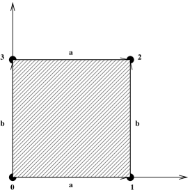
Figure 1. Concurrent execution of two actions $a$ and $b$

In the combinatorial semantics, the preceding situation is abstracted by a $2$-cube viewed as a precubical set. Let us now recall the definition of these objects. A good reference for presheaves is [MLM94].

2.1 Notation.

Let $[0]=\{0\}$ and $[n]=\{0,1\}^{n}$ for $n\geqslant 1$. By convention, $\{0,1\}^{0}=\{0\}$.

Let $\delta_{i}^{\alpha}:[n-1]\rightarrow[n]$ be the set map defined for $1\leqslant i\leqslant n$ and $\alpha\in\{0,1\}$ by $\delta_{i}^{\alpha}(\epsilon_{1},\dots,\epsilon_{n-1})=(\epsilon_{1},\dots,\epsilon_{i-1},\alpha,\epsilon_{i},\dots,\epsilon_{n-1})$. The small category $\square$ is by definition the subcategory of the category of sets with set of objects $\{[n],n\geqslant 0\}$ and generated by the morphisms $\delta_{i}^{\alpha}$.

2.2 Definition.

[BH81] The category of presheaves over $\square$, denoted by $\square^{op}{\rm{\mathbf{Set}}}$, is called the category of precubical sets. A precubical set $K$ consists of a family of sets $(K_{n})_{n\geqslant 0}$ and of set maps $\partial_{i}^{\alpha}:K_{n}\rightarrow K_{n-1}$ with $1\leqslant i\leqslant n$ and $\alpha\in\{0,1\}$ satisfying the cubical relations $\partial_{i}^{\alpha}\partial_{j}^{\beta}=\partial_{j-1}^{\beta}\partial_{i}^{\alpha}$ for any $\alpha,\beta\in\{0,1\}$ and for $i<j$. An element of $K_{n}$ is called a $n$-cube.

Let $\square[n]:=\square(-,[n])$. By the Yoneda lemma, one has the natural bijection of sets

$$\square^{op}{\rm{\mathbf{Set}}}(\square[n],K)\cong K_{n}$$

for every precubical set $K$. The boundary of $\square[n]$ is the precubical set denoted by $\partial\square[n]$ defined by removing the interior of $\square[n]$:

• $(\partial\square[n])_{k}:=(\square[n])_{k}$ for $k<n$

• $(\partial\square[n])_{k}=\varnothing$ for $k\geqslant n$.

In particular, one has $\partial\square[0]=\varnothing$.

So the $2$-cube $\square[2]$ models the underlying time flow of the concurrent execution of $a$ and $b$. However, the same $2$-cube models the underlying time flow of the concurrent execution of any pair of actions. So we need a notion of labelling.

Let $\Sigma$ be a set of labels, containing among other things the two actions $a$ and $b$.

2.3 Proposition.

[Gou02] Put a total ordering $\leqslant$ on $\Sigma$. Let

• $(!\Sigma)_{0}=\{()\}$ (the empty word)

• for $n\geqslant 1$, $(!\Sigma)_{n}=\{(a_{1},\dots,a_{n})\in\Sigma\times\dots\times\Sigma,a_{1}\leqslant\dots\leqslant a_{n}\}$

• $\partial_{i}^{0}(a_{1},\dots,a_{n})=\partial_{i}^{1}(a_{1},\dots,a_{n})=(a_{1},\dots,\widehat{a_{i}},\dots,a_{n})$ where the notation $\widehat{a_{i}}$ means that $a_{i}$ is removed.

Then these data generate a precubical set.

2.4 Remark.

The isomorphism class of $!\Sigma$ does not depend of the choice of the total ordering on $\Sigma$.

2.5 Definition.

(Goubault) A labelled precubical set is an object of the comma category $\square^{op}{\rm{\mathbf{Set}}}{\downarrow}!\Sigma$.

In the combinatorial semantics, the concurrent action of the two actions $a$ and $b$ is then modeled by the labelled $2$-cube $\ell:\square[2]\rightarrow!\Sigma$ sending the identity of $[2]$ (the interior of the square) to $(a,b)$ if $a\leqslant b$ or to $(b,a)$ if $b\leqslant a$ as depicted in Figure 2.

Figure 2. Concurrent execution of $a$ and $b$ with $a\leqslant b$ as labelled precubical set

The categorical semantics is much simpler to explain. Each of the four distinguished states $0$, $1$, $2$ and $3$ of Figure 1 is represented by an object of a small category. Each execution path of the boundary of the square is represented by a morphism with the composition of execution paths corresponding to the composition of morphisms. So one has $6$ execution paths $\overrightarrow{01}$, $\overrightarrow{12}$, $\overrightarrow{012}$, $\overrightarrow{03}$, $\overrightarrow{32}$ and $\overrightarrow{032}$ with the algebraic rules $\overrightarrow{01}*\overrightarrow{12}=\overrightarrow{012}$ and $\overrightarrow{03}*\overrightarrow{32}=\overrightarrow{032}$ where $*$ is of course the composition law. The interior of the square is then modeled by the algebraic relation $\overrightarrow{012}=\overrightarrow{032}$. This small category is nothing else but the small category corresponding to the poset $\{\widehat{0}<\widehat{1}\}^{2}$. And this poset is nothing else but the poset of vertices of the $2$-cube. The partial ordering models observable time ordering.

In fact, one needs to work with categories enriched over topological spaces in the sense of [Kel05], i.e. with topologized homsets, for being able to model more complicated situations of concurrency. In the situation above, the space of morphisms is of course discrete. For various mathematical reasons, e.g. [Gau03] Section 20 and [GG03] Section 6, one also needs to work with small category without identity maps. Note that the category of small categories without identity maps and the usual one of small categories are certainly not equivalent since a round-trip using the adjunction between them adds a loop to each object. And a lots of theorems proved in the framework of flows (i.e. small categories without identity maps enriched over topological spaces) are merely wrong whenever identity maps are added.

In this paper, one will also work with the locally presentable category of $\Delta$-generated topological spaces, denoted by ${\mathbf{Top}}$, i.e. of spaces which are colimits of simplices. Several introductions about these topological spaces are available in [Dug03] [FR07] and [Gau07b] respectively. Let us only mention one striking property of $\Delta$-generated topological spaces: as the simplicial sets, they are isomorphic to the disjoint sum of their [path-]connected components by [Gau07b] Proposition 2.8. This property has a lots of very nice consequences.

2.6 Definition.

[Gau03] A flow $X$ is a small category without identity maps enriched over $\Delta$-generated topological spaces. The composition law of a flow is denoted by $*$. The set of objects is denoted by $X^{0}$. The space of morphisms from $\alpha$ to $\beta$ is denoted by $\mathbb{P}_{\alpha,\beta}X$ . Let $\mathbb{P}X$ be the disjoint sum of the spaces $\mathbb{P}_{\alpha,\beta}X$. A morphism of flows $f:X\rightarrow Y$ is a set map $f^{0}:X^{0}\rightarrow Y^{0}$ together with a continuous map $\mathbb{P}f:\mathbb{P}X\rightarrow\mathbb{P}Y$ preserving the structure. The corresponding category is denoted by ${\rm{\mathbf{Flow}}}$.

Each poset $P$ can be associated with a flow denoted in the same way. The set of objects $P^{0}$ is the underlying set of $P$ and there is one and only one morphism from $\alpha$ to $\beta$ if and only if $\alpha<\beta$. The composition law is then defined by $(\alpha,\beta)*(\beta,\gamma)=(\alpha,\gamma)$ for any $\alpha<\beta<\gamma\in P$. Note that the flow associated with a poset is loopless, i.e. for every $\alpha\in P^{0}$, one has $\mathbb{P}_{\alpha,\alpha}P=\varnothing$. This construction induces a functor ${\rm{\mathbf{PoSet}}}\rightarrow{\rm{\mathbf{Flow}}}$ from the category of posets together with the strictly increasing maps to the category of flows.

In the categorical semantics, the underlying time flow of the concurrent execution of two actions $a$ and $b$ is then modeled by the flow associated with the poset $\{\widehat{0}<\widehat{1}\}^{2}$. Like in the combinatorial semantics, one needs a notion of labelling.

2.7 Definition.

The flow of labels $?\Sigma$ is defined as follows: $(?\Sigma)^{0}=\{0\}$ and $\mathbb{P}?\Sigma$ is the discrete free associative monoid without unit generated by the elements of $\Sigma$ and by the algebraic relations $a*b=b*a$ for all $a,b\in\Sigma$.

2.8 Definition.

A labelled flow is an object of the comma category ${\rm{\mathbf{Flow}}}{\downarrow}?\Sigma$.

So the concurrent execution of the two actions $a$ and $b$ will be modeled by the labelled flow $\ell:\{\widehat{0}<\widehat{1}\}^{2}\rightarrow?\Sigma$ with $\ell(\overrightarrow{012})=\ell(\overrightarrow{032})=a*b$, $\ell(\overrightarrow{01})=a$, $\ell(\overrightarrow{12})=b$, $\ell(\overrightarrow{03})=b$ and $\ell(\overrightarrow{32})=a$ as in Figure 3.

Figure 3. Concurrent execution of $a$ and $b$ as labelled flow

3. Combinatorial semantics of CCS

Syntax of the process algebra CCS

A short introduction about process algebra can be found in [WN95]. An introduction about CCS for mathematician is available in the companion paper [Gau07c]. Let $\Sigma$ be a non-empty set. Its elements are called labels or actions or events. From now on, the set $\Sigma$ is supposed to be equipped with an involution $a\mapsto\overline{a}$. Moreover, the set $\Sigma$ contains a distinct action $\tau$ with $\tau=\overline{\tau}$. The process names are generated by the following syntax:

$$P::=nil\ |\ a.P\ |\ (\nu a)P\ |\ P+P\ |\ P||P\ |\ \operatorname{rec}(x)P(x)$$

where $P(x)$ means a process name with one free variable $x$. The variable $x$ must be guarded, that is it must lie in a prefix term $a.x$ for some $a\in\Sigma$.

Parallel composition with synchronization of labelled precubical sets

3.1 Definition.

Let $\ell:K\rightarrow!\Sigma$ be a labelled precubical set. Let $n\geqslant 1$. A labelled $n$-shell of $K$ is a commutative diagram of precubical sets

Suppose moreover that $K_{0}=[p]$ for some $p\geqslant 2$. The labelled $n$-shell above is non-twisted if the set map $x_{0}:[n+1]=\partial\square[n+1]_{0}\rightarrow[p]=K_{0}$ is a composite

$$x_{0}:[n+1]\stackrel{{\scriptstyle\phi}}{{\longrightarrow}}[q]\stackrel{{\scriptstyle\psi}}{{\longrightarrow}}[p]$$

where $\psi$ is a morphism of the small category $\square$ and where $\phi$ is of the form $(\epsilon_{1},\dots,\epsilon_{n+1})\mapsto(\epsilon_{i_{1}},\dots,\epsilon_{i_{q}})$ such that $1=i_{1}\leqslant\dots\leqslant i_{q}=n+1$ and $\{1,\dots,n+1\}\subset\{i_{1},\dots,i_{q}\}$.

The map $\phi$ is not necessarily a morphism of the small category $\square$. For example $\phi:[3]\rightarrow[5]$ defined by $\phi(\epsilon_{1},\epsilon_{2},\epsilon_{3})=(\epsilon_{1},\epsilon_{1},\epsilon_{2},\epsilon_{3},\epsilon_{3})$ is not a morphism of $\square$. Note the set map $x_{0}$ is always one-to-one.

All labelled shells of this paper will be supposed non-twisted.

3.2 Definition.

Let $\square_{n}\subset\square$ be the full subcategory of $\square$ whose set of objects is $\{[k],k\leqslant n\}$. The category of presheaves over $\square_{n}$ is denoted by $\square_{n}^{op}{\rm{\mathbf{Set}}}$. Its objects are called the $n$-dimensional precubical sets.

Let $K$ be an object of $\square_{1}^{op}{\rm{\mathbf{Set}}}{\downarrow}!\Sigma$ such that $K_{0}=[p]$ for some $p\geqslant 2$. Let $K^{(n)}$ be the object of $\square_{n}^{op}{\rm{\mathbf{Set}}}{\downarrow}!\Sigma$ inductively defined for $n\geqslant 1$ by $K^{(1)}=K$ and by the following pushout diagram of labelled precubical sets (the shells are always non-twisted by hypothesis):

Since $(\partial\square[n+1])_{p}=(\square[n+1])_{p}$ for $p\leqslant n$, one has $(K^{(n+1)})_{p}=(K^{(n)})_{p}$ for $p\leqslant n$. And by construction, $(K^{(n+1)})_{n+1}$ is the set of non-twisted labelled $n$-shell of $K$. There is an inclusion map $K^{(n)}\rightarrow K^{(n+1)}$.

3.3 Notation.

Let $K$ be a $1$-dimensional labelled precubical set with $K_{0}=[p]$ for some $p\geqslant 2$. Then let

$$\operatorname{COSK}(K):=\varinjlim_{n\geqslant 1}K^{(n)}.$$

The important property of the $\operatorname{COSK}$ operator, also used in the proof of Proposition 6.5, is the following one ensuring that the higher dimensional automata paradigm is satisfied indeed:

3.4 Proposition.

([Gau07c] Proposition 3.16) Let $\square[n]$ be a labelled precubical set with $n\geqslant 2$. Then one has the isomorphism of labelled precubical sets $\operatorname{COSK}(\square[n]_{\leqslant 1})\cong\square[n]$.

Roughly speaking, Proposition 3.4 states that for all $1\leqslant p\leqslant n-1$, there is a bijection between the non-twisted labelled $p$-shells of $\square[n]$ and the $(p+1)$-cubes of $\square[n]$. If the condition non-twisted is removed, i.e. if we work with a too naive notion of labelled coskeleton construction as in [Wor04], then Proposition 3.4 is no longer true. Indeed, a naive labelled coskeleton construction adds too many cubes whereas the higher dimensional automata paradigm states that one must recover exactly $\square[n]$ from $\square[n]_{\leqslant 1}$ which corresponds to the concurrent execution of $n$ actions. That was the problem in K. Worytkiewicz’s coskeleton construction, which was corrected in the companion paper [Gau07c].

3.5 Definition.

Let $K$ and $L$ be two labelled precubical sets. The synchronized tensor product is by definition

$$K\otimes_{\sigma}L:=\varinjlim_{\square[m]\rightarrow K}\varinjlim_{\square[n]\rightarrow L}\operatorname{COSK}(Z)$$

where $Z$ is the $1$-dimensional precubical set defined by:

• $Z_{0}:=\square[m]_{0}\times\square[n]_{0}$

• $Z_{1}:=(\square[m]_{1}\times\square[n]_{0})\oplus(\square[m]_{0}\times\square[n]_{1})\oplus\{(x,y)\in\square[m]_{1}\times\square[n]_{1},\overline{\ell(x)}=\ell(y)\}$ with an obvious definition of the face maps and the labelling $\tau=\ell(x,y)$ if $\overline{\ell(x)}=\ell(y)$.

Construction of the labelled precubical set of paths

3.6 Definition.

A labelled precubical set $\ell:K\rightarrow!\Sigma$ decorated by process names is a labelled precubical set together with a set map $d:K_{0}\rightarrow{\rm{\mathbf{Proc}}}_{\Sigma}$ called the decoration.

It is recalled in Table 1 the construction of the labelled precubical set $\square\llbracket P\rrbracket$ of [Gau07c] by induction on the syntax of the name. The labelled precubical set $\square\llbracket P\rrbracket$ has a unique initial state canonically decorated by the process name $P$ and its other states will be decorated as well in an inductive way. Therefore for every process name $P$, $\square\llbracket P\rrbracket$ is an object of $\{i\}{\downarrow}\square^{op}{\rm{\mathbf{Set}}}{\downarrow}!\Sigma$.

$\square\llbracket nil\rrbracket:=\square[0]$

$\square\llbracket\mu.nil\rrbracket:=\mu.nil\stackrel{{\scriptstyle(\mu)}}{{\longrightarrow}}nil$

$\square\llbracket P+Q\rrbracket:=\square\llbracket P\rrbracket\oplus\square\llbracket Q\rrbracket$

with the binary coproduct taken in $\{i\}{\downarrow}\square^{op}{\rm{\mathbf{Set}}}{\downarrow}!\Sigma$

$\square\llbracket P||Q\rrbracket:=\square\llbracket P\rrbracket\otimes_{\sigma}\square\llbracket Q\rrbracket$

$\square\llbracket\operatorname{rec}(x)P(x)\rrbracket:=\varinjlim\limits_{n}\square\llbracket P^{n}(nil)\rrbracket$

Table 1. Combinatorial semantics of CCS

4. Categorical semantics of CCS

The categorical semantics of CCS is obtained from the combinatorial semantics by applying the geometric realization functor $|-|:\square^{op}{\rm{\mathbf{Set}}}\rightarrow{\rm{\mathbf{Flow}}}$ introduced in [Gau07c] . As already explained in [Gau07c], it is necessary to use the model structure introduced in [Gau03], and adapted in [Gau07b] for the framework of $\Delta$-generated topological spaces. Equivalent geometric realization functors are defined in [Gau07a]. We will use the construction of [Gau07c] in this paper.

Let $Z$ be a topological space. The flow ${\rm{Glob}}(Z)$ is defined by

• ${\rm{Glob}}(Z)^{0}=\{\widehat{0},\widehat{1}\}$,

• $\mathbb{P}{\rm{Glob}}(Z)=\mathbb{P}_{\widehat{0},\widehat{1}}{\rm{Glob}}(Z)=Z$,

• $s=\widehat{0}$, $t=\widehat{1}$ and a trivial composition law.

It is called the globe of the space $Z$.

The model structure of [Gau07b] is characterized as follows:

• The weak equivalences are the weak S-homotopy equivalences, i.e. the morphisms of flows $f:X\longrightarrow Y$ such that $f^{0}:X^{0}\longrightarrow Y^{0}$ is a bijection of sets and such that $\mathbb{P}f:\mathbb{P}X\longrightarrow\mathbb{P}Y$ is a weak homotopy equivalence.

• The fibrations are the morphisms of flows $f:X\longrightarrow Y$ such that $\mathbb{P}f:\mathbb{P}X\longrightarrow\mathbb{P}Y$ is a Serre fibration.

This model structure is cofibrantly generated. The set of generating cofibrations is the set $I^{gl}_{+}=I^{gl}\cup\{R:\{0,1\}\longrightarrow\{0\},C:\varnothing\longrightarrow\{0\}\}$ with

$$\boxed{I^{gl}=\{{\rm{Glob}}(\mathbf{S}^{n-1})\subset{\rm{Glob}}(\mathbf{D}^{n}),n\geqslant 0\}}$$

where $\mathbf{D}^{n}$ is the $n$-dimensional disk and $\mathbf{S}^{n-1}$ the $(n-1)$-dimensional sphere. By convention, the $(-1)$-dimensional sphere is the empty space. The set of generating trivial cofibrations is

$$\boxed{J^{gl}=\{{\rm{Glob}}(\mathbf{D}^{n}\times\{0\})\subset{\rm{Glob}}(\mathbf{D}^{n}\times[0,1]),n\geqslant 0\}}.$$

The mapping from $\operatorname{Obj}(\square)$ (the set of objects of $\square$) to $\operatorname{Obj}({\rm{\mathbf{Flow}}})$ (the class of flows) defined by $[0]\mapsto\{0\}$ and $[n]\mapsto\{\widehat{0}<\widehat{1}\}^{n}$ for $n\geqslant 1$ induces a functor from the category $\square$ to the category ${\rm{\mathbf{Flow}}}$ by composition

$$\square\subset{\rm{\mathbf{PoSet}}}\longrightarrow{\rm{\mathbf{Flow}}}.$$

4.1 Notation.

A state of the flow $\{\widehat{0}<\widehat{1}\}^{n}$ is denoted by a $n$-uple of elements of $\{\widehat{0},\widehat{1}\}$. The unique morphism/execution path from $(x_{1},\dots,x_{n})$ to $(y_{1},\dots,y_{n})$ is denoted by a $n$-uple $(z_{1},\dots,z_{n})$ with $z_{i}=x_{i}$ if $x_{i}=y_{i}$ and $z_{i}=*$ if $x_{i}<y_{i}$. For example in the flow $\{\widehat{0}<\widehat{1}\}^{2}$ depicted in Figure 4, one has the algebraic relation $(*,*)=(\widehat{0},*)*(*,\widehat{1})=(*,\widehat{0})*(\widehat{1},*)$.

4.2 Definition.

[Gau07c] Let $K$ be a precubical set. By definition, the geometric realization of $K$ is the flow

$$\boxed{|K|:=\varinjlim_{\square[n]\rightarrow K}(\{\widehat{0}<\widehat{1}\}^{n})^{cof}}.$$

The following proposition is helpful to understand what this geometric realization functor is. The principle of its proof will be reused in the paper.

4.3 Proposition.

Let $K$ be a precubical set. One has a natural weak S-homotopy equivalence

$$|K|\simeq\mathop{\mathchoice{\vtop{\halign{#\cr\hfil$\displaystyle\operator@font holim$\hfil\cr\nointerlineskip\kern 1.5pt\cr\rightarrowfill@\textstyle\cr\nointerlineskip\kern-1.0pt\cr\cr}}}{\vtop{\halign{#\cr\hfil$\textstyle\operator@font holim$\hfil\cr\nointerlineskip\kern 1.5pt\cr\rightarrowfill@\textstyle\cr\nointerlineskip\kern-1.0pt\cr\cr}}}{\vtop{\halign{#\cr\hfil$\scriptstyle\operator@font holim$\hfil\cr\nointerlineskip\kern 1.5pt\cr\rightarrowfill@\textstyle\cr\nointerlineskip\kern-1.0pt\cr\cr}}}{\vtop{\halign{#\cr\hfil$\scriptscriptstyle\operator@font holim$\hfil\cr\nointerlineskip\kern 1.5pt\cr\rightarrowfill@\textstyle\cr\nointerlineskip\kern-1.0pt\cr\cr}}}}\displaylimits_{\square[n]\rightarrow K}\{\widehat{0}<\widehat{1}\}^{n}.$$

Proof.

Consider the category of cubes $\square{\downarrow}K$ of $K$. It is defined by the pullback diagram of small categories

In other terms, an object of $\square{\downarrow}K$ is a morphism $\square[m]\rightarrow K$ and a morphism of $\square{\downarrow}K$ is a commutative diagram

The category $\square{\downarrow}K$ is a Reedy direct category with the degree function $d(\square[n]\rightarrow K)=n$. Since this Reedy category is direct, the matching category is always empty. So by [Hir03] Proposition 15.10.2, the Reedy category has fibrant constants and the colimit functor $\varinjlim:{\rm{\mathbf{Flow}}}^{\square{\downarrow}K}\rightarrow{\rm{\mathbf{Flow}}}$ is a left Quillen functor if ${\rm{\mathbf{Flow}}}^{\square{\downarrow}K}$ is equipped with the Reedy model structure by [Hir03] Theorem 15.10.8. Consider the functor $D:\square{\downarrow}K\rightarrow{\rm{\mathbf{Flow}}}$ defined by $D(\square[n]\rightarrow K):=(\{\widehat{0}<\widehat{1}\}^{n})^{cof}$. One has to check that the diagram $D$ is Reedy cofibrant and the proof will be complete. By definition of the Reedy model structure, it suffices to show that for all $n\geqslant 0$, and with $\alpha=\square[n]\rightarrow K$, the map $L_{\alpha}D\rightarrow D(\alpha)$ is a cofibration where $L_{\alpha}D$ is the latching object at $\alpha$. It is easy to see that the latter map is the morphism of flows $|\partial\square[n]\subset\square[n]|$ which is a cofibration of flows by Theorem 4.5 below. ∎

Figure 4. The flow $|\square[2]|_{bad}=\{\widehat{0}<\widehat{1}\}^{2}$ ($(*,*)=(\widehat{0},*)*(*,\widehat{1})=(*,\widehat{0})*(\widehat{1},*)$)

The functor $[n]\mapsto\{\widehat{0}<\widehat{1}\}^{n}$ from $\square$ to ${\rm{\mathbf{Flow}}}$ also induces a bad realization functor from $\square^{op}{\rm{\mathbf{Set}}}$ to ${\rm{\mathbf{Flow}}}$ defined by

$$\boxed{|K|_{bad}:=\varinjlim_{\square[n]\rightarrow K}\{\widehat{0}<\widehat{1}\}^{n}}.$$

This functor is a bad realization because of the following bad behaviour:

4.4 Theorem.

([Gau07c] Theorem 7.2) Let $n\geqslant 3$. The inclusion of precubical sets $\partial\square[n]\subset\square[n]$ induces an isomorphism $|\partial\square[n]|_{bad}\cong|\square[n]|_{bad}$.

On the contrary, the geometric realization functor is well-behaved:

4.5 Theorem.

([Gau07c] Proposition 7.6 and [Gau07c] Theorem 7.8) For any $n\geqslant 0$, the map of flows $|\partial\square[n]\subset\square[n]|$ is a non-trivial cofibration of flows. Moreover, the path space $\mathbb{P}_{\widehat{0}\dots\widehat{0},\widehat{1}\dots\widehat{1}}|\partial\square[n]|$ is homotopy equivalent to $\mathbf{S}^{n-2}$ and the path space $\mathbb{P}_{\widehat{0}\dots\widehat{0},\widehat{1}\dots\widehat{1}}|\square[n]|$ is contractible.

Let $K\rightarrow!\Sigma$ be a labelled precubical set. Then the composition $|K|\rightarrow|!\Sigma|\rightarrow|!\Sigma|_{bad}\cong?\Sigma$ gives rise to a labelled flow by [Gau07c] Proposition 8.1.

4.6 Notation.

For every process name $P$, let $\llbracket P\rrbracket:=|\square\llbracket P\rrbracket|$. The flow $\llbracket P\rrbracket$ is always cofibrant by [Gau07c] Proposition 7.7.

Note that a decorated labelled precubical set gives rise to a decorated labelled flow in the following sense:

4.7 Definition.

A labelled flow $\ell:X\rightarrow?\Sigma$ decorated by process names is a labelled flow together with a set map $d:X^{0}\rightarrow{\rm{\mathbf{Proc}}}_{\Sigma}$ called the decoration.

5. Relevance of weak S-homotopy for concurrency theory

The translation of the combinatorial semantics of CCS into a categorical semantics in terms of flows requires the use of non-canonical constructions, more precisely, a non-canonical choice of a cofibrant replacement functor, and also later non-canonical choices for homotopy limits and homotopy colimits. The following theorem is therefore very important:

5.1 Theorem.

For any flow $X$, there exists at most one precubical set $K$ up to isomorphism such that $|K|\simeq X$. In other terms, the functor

$$K\mapsto\hbox{weak S-homotopy type of }|K|$$

from $\square^{op}{\rm{\mathbf{Set}}}$ to the homotopy category of flows ${\mathbf{Ho}}({\rm{\mathbf{Flow}}})$ reflects isomorphisms.

The precubical set $K$ does not necessarily exist. For example, ${\rm{Glob}}(\mathbf{S}^{1})$ is not weakly S-homotopy equivalent to any geometric realization of any precubical set. Indeed, if there existed a precubical set $K$ with $|K|\simeq{\rm{Glob}}(\mathbf{S}^{1})$, then $K$ would have a unique initial state $\widehat{0}$ and a unique final state $\widehat{1}$, so $K_{0}=\{\widehat{0},\widehat{1}\}$. So the only possibility is a set of $1$-cubes from $\widehat{0}$ to $\widehat{1}$. Thus the space $\mathbb{P}(|K|)$ would be homotopy equivalent to a discrete space.

Before proving Theorem 5.1, we need to establish several preliminary results involving among other things the simplicial structure of the category of flows.

In any flow $X$, if two execution paths $x$ and $y$ are in the same path-connected component of some $\mathbb{P}_{\alpha,\beta}X$, then there exists a continuous map $\phi:[0,1]\rightarrow\mathbb{P}_{\alpha,\beta}X$ with $\phi(0)=x$ and $\phi(1)=y$. So for any execution path $z$ such that $x*z$ and $y*z$ exist, the continuous map $\psi$ from $[0,1]$ to $\mathbb{P}X$ defined by $\psi(t)=\phi(t)*z$ is a continuous path from $x*z$ to $y*z$. Hence:

5.2 Notation.

Any flow $X$ induces a flow over the category of sets denoted by $\widehat{\pi}_{0}(X)$ defined by $\widehat{\pi}_{0}(X)^{0}=X^{0}$, $\mathbb{P}\widehat{\pi}_{0}(X)=\pi_{0}(\mathbb{P}X)$ where $\pi_{0}$ is the path-connected component functor and with the composition law induced by the one of $X$.

5.3 Notation.

Let ${\rm{\mathbf{Flow}}}({\rm{\mathbf{Set}}})$ be the category of flows enriched over sets, i.e. of small categories without identity maps.

5.4 Proposition.

The functor $\widehat{\pi}_{0}:{\rm{\mathbf{Flow}}}\rightarrow{\rm{\mathbf{Flow}}}({\rm{\mathbf{Set}}})$ is a left adjoint. In particular, it is colimit-preserving.

Proof.

It suffices to prove that the path-connected component functor $\pi_{0}:{\mathbf{Top}}\rightarrow{\rm{\mathbf{Set}}}$ is a left adjoint (let us repeat that we are working with $\Delta$-generated topological spaces). Here are two possible arguments:

1. Every space is homeomorphic to the disjoint sum of its path-connected components by [Gau07b] Proposition 2.8. In fact, a space is even connected if and only if it is path-connected. So it is easy to see that the right adjoint is the functor from ${\rm{\mathbf{Set}}}$ to ${\mathbf{Top}}$ taking a set $S$ to the discrete space $S$.

2. The functor from ${\rm{\mathbf{Set}}}$ to ${\mathbf{Top}}$ taking a set $S$ to the discrete space $S$ commutes with limits because there is no non-discrete totally disconnected $\Delta$-generated spaces, and with colimits as in the category of general topological spaces. In particular it is accessible. So by [AR94] Theorem 1.66, it has a left adjoint and it is easy to see that the left adjoint is the path-connected component functor.

∎

5.5 Proposition.

(Compare with [Gau07b] Proposition 4.9) The path space functor $\mathbb{P}:{\rm{\mathbf{Flow}}}\rightarrow{\mathbf{Top}}$ is a right adjoint. In particular, it is accessible.

In fact, the functor $\mathbb{P}:{\rm{\mathbf{Flow}}}\rightarrow{\mathbf{Top}}$ is of course finitely accessible.

Proof.

Let $Z$ be a topological space. By [Gau07b] Proposition 2.8, $Z$ is homeomorphic to the disjoint union of its path-connected components. Let us write this situation by

$$Z\cong\bigsqcup_{Z_{i}\in\pi_{0}(Z)}Z_{i}.$$

Then one has for any flow $X$

$${\mathbf{Top}}(Z,\mathbb{P}X) \cong \prod_{Z_{i}\in\pi_{0}(Z)}{\mathbf{Top}}(Z_{i},\mathbb{P}X)$$

$$\cong \prod_{Z_{i}\in\pi_{0}(Z)}{\rm{\mathbf{Flow}}}({\rm{Glob}}(Z_{i}),X)$$

$$\cong {\rm{\mathbf{Flow}}}(\bigsqcup_{Z_{i}\in\pi_{0}(Z)}{\rm{Glob}}(Z_{i}),X).$$

So the path space functor $\mathbb{P}:{\rm{\mathbf{Flow}}}\rightarrow{\mathbf{Top}}$ is accessible by [AR94] Theorem 1.66. ∎

5.6 Proposition.

Let $i:A\rightarrow X$ be a cofibration of flows between cofibrant flows. Then the continuous map $\mathbb{P}i:\mathbb{P}A\rightarrow\mathbb{P}X$ is a cofibration between cofibrant spaces.

Note that Proposition 5.6 remains true if we only suppose that the space $\mathbb{P}A$ is cofibrant. Proposition 5.6 is a generalization of [Gau07b] Proposition 7.5.

Proof.

Let us suppose first that there is a pushout diagram of flows

By [Gau03] Proposition 15.1, the continuous map $\mathbb{P}i:\mathbb{P}A\rightarrow\mathbb{P}X$ is a transfinite composition of pushouts of maps of the form $\operatorname{Id}_{X_{1}}\times\dots\times i_{n}\times\dots\times\operatorname{Id}_{X_{p}}$ where the spaces $X_{i}$ are spaces of the form $\mathbb{P}_{\alpha,\beta}A$ and where $i_{n}:\mathbf{S}^{n-1}\subset\mathbf{D}^{n}$ is the inclusion with $n\geqslant 0$. Any space of the form $\mathbb{P}_{\alpha,\beta}A$ is cofibrant by [Gau07b] Proposition 7.5 since $A$ is cofibrant. So the map $\mathbb{P}i:\mathbb{P}A\rightarrow\mathbb{P}X$ is a cofibration because the model category $({\mathbf{Top}},\times)$ is monoidal.

Let us treat now the general case. The cofibration $i$ is a retract of a map $j:A\rightarrow Y$ of $\operatorname{{\rm{\mathbf{cell}}}}(I^{gl}_{+})$ by a map which fixes $A$ by [Hov99] Corollary 2.1.15. So the continuous map $\mathbb{P}i:\mathbb{P}A\rightarrow\mathbb{P}X$ is a retract of the continuous map $\mathbb{P}j:\mathbb{P}A\rightarrow\mathbb{P}Y$. The map of flows $j:A\rightarrow Y$ is the composition of a transfinite sequence $Z:\lambda\rightarrow{\rm{\mathbf{Flow}}}$ for some ordinal $\lambda$ with $Z_{0}=A$. By Proposition 5.5, one has the homeomorphism $\varinjlim\mathbb{P}Z_{\alpha}\cong\mathbb{P}Y$. The first part of this proof implies that $\mathbb{P}j:\mathbb{P}A\rightarrow\mathbb{P}Y$ is then a cofibration of spaces, and therefore that $\mathbb{P}i:\mathbb{P}A\rightarrow\mathbb{P}X$ is a cofibration as well. ∎

5.7 Notation.

The associative monoid without unit $(\mathbb{N}^{*},+)$ of strictly positive integers together with the addition can be viewed as a flow with one object, the discrete path space $\mathbb{N}^{*}$ and the composition law $+$.

5.8 Notation.

Let $K$ be a precubical set. Let $K_{\leqslant n}$ be the precubical set obtained from $K$ by keeping the $p$-dimensional cubes of $K$ only for $p\leqslant n$. In particular, $K_{\leqslant 0}=K_{0}$.

5.9 Proposition.

Let $K$ be a precubical set. There exists a unique morphism of flows $L_{K}:\widehat{\pi}_{0}(|K|)\rightarrow\mathbb{N}^{*}$, natural with respect to $K$, such that for any $x\in K_{1}$, for any $z\in\mathbb{P}(|\square[1]|)$, one has $L_{K}(|x|(z))=1$.

Proof.

We construct $L_{K}:\widehat{\pi}_{0}(|K_{\leqslant n}|)\rightarrow\mathbb{N}^{*}$ for any precubical set $K$ by induction on $n\geqslant 0$. There is nothing to do for $n=0$. The passage from $|K_{\leqslant n}|$ to $|K_{\leqslant n+1}|$ is done as usual by the following pushout diagram of flows:

where the sum is over all $n$-shells $x:\partial\square[n+1]\subset\square[n+1]\rightarrow K$. Let $n\geqslant 0$. By induction hypothesis, the flow $\widehat{\pi}_{0}(|\partial\square[n+1]|)$ and $\widehat{\pi}_{0}(|K_{\leqslant n}|)$ are defined. We know that the map of flows $|\partial\square[n+1]|\rightarrow|\square[n+1]|$ is a cofibration by Theorem 4.5. In fact, this map of flows induces the identity maps $\mathbb{P}_{\alpha,\beta}(|\partial\square[n+1]|)=\mathbb{P}_{\alpha,\beta}(|\square[n+1]|)$ for $(\alpha,\beta)\neq(\widehat{0}\dots\widehat{0},\widehat{1}\dots\widehat{1})$ and a non-trivial cofibration  between cofibrant spaces $\mathbb{P}_{\widehat{0}\dots\widehat{0},\widehat{1}\dots\widehat{1}}(|\partial\square[n+1]|)\rightarrow\mathbb{P}_{\widehat{0}\dots\widehat{0},\widehat{1}\dots\widehat{1}}(|\square[n+1]|)$ by Proposition 5.6. Then let $L_{\square[n+1]}(x)=n+1$ for any $x\in\mathbb{P}_{\widehat{0}\dots\widehat{0},\widehat{1}\dots\widehat{1}}(|\square[n+1]|)$. One obtains the commutative square of ${\rm{\mathbf{Flow}}}({\rm{\mathbf{Set}}})$:

By Proposition 5.4 and by the universal property of the pushout, one obtains the natural map $\widehat{\pi}_{0}(|K_{\leqslant n+1}|)\rightarrow\mathbb{N}^{*}$. Since the functor $K\mapsto\widehat{\pi}_{0}(|K|)$ is a left adjoint, one obtains a natural map $\widehat{\pi}_{0}(|K|)\cong\varinjlim\widehat{\pi}_{0}(|K_{\leqslant n}|)\rightarrow\mathbb{N}^{*}$. ∎

5.10 Definition.

The integer $L_{K}(x)$ for $x\in\mathbb{P}(|K|)$ is called the length of $x$.

Proposition 5.9 means that the length of $x\in\mathbb{P}(|K|)$ satisfies the following (intuitive) algebraic rules:

• $L_{K}(x*y)=L_{K}(x)+L_{K}(y)$ if $x$ and $y$ are composable

• $L_{K}(x)=L_{K}(y)$ if $x$ and $y$ are in the same path-connected component of the space $\mathbb{P}(|K|)$

• $L_{K}(x)=1$ if $x$ corresponds to an edge, i.e. a $1$-cube, of the precubical set $K$

• the naturality of the morphism of flows $L_{K}:\widehat{\pi}_{0}(|K|)\rightarrow\mathbb{N}^{*}$ means that length is preserved by a map of precubical sets.

The model category ${\rm{\mathbf{Flow}}}$ is simplicial by [Gau07a] Section 3 and [Gau07b] Appendix B. Let $\operatorname{Map}(X,Y)$ be the function complex from $X$ to $Y$. It is equal to the simplicial nerve of the space ${\rm{\mathbf{FLOW}}}(X,Y)$ of morphisms of flows from $X$ to $Y$ equipped with the Kelleyfication of the relative topology.

5.11 Proposition.

Let $K$ be a precubical set. Let $n\geqslant 0$. The natural set map $K_{n}\rightarrow{\rm{\mathbf{Flow}}}(|\square[n]|,|K|)$ defined by taking $x\in K_{n}$ to $|x|:|\square[n]|\rightarrow|K|$ is one-to-one.

Proof.

One has $|K|=\varinjlim_{\square[n]\rightarrow K}|\square[n]|$ by definition. If $x$ and $y$ are two different $n$-cubes of $K$, then they correspond to two different copies of $|\square[n]|$ in the colimit calculating $K$. Let

$$\gamma\in\mathbb{P}_{\widehat{0}\dots\widehat{0},\widehat{1}\dots\widehat{1}}|\square[n]|\backslash\mathbb{P}_{\widehat{0}\dots\widehat{0},\widehat{1}\dots\widehat{1}}|\partial\square[n]|.$$

Then $|x|(\gamma)\neq|y|(\gamma)$. Therefore $|x|\neq|y|$. ∎

5.12 Notation.

Let $K$ be a precubical set. The precubical set $\widehat{K}$ is defined by

$$\boxed{\widehat{K}=\pi_{0}\operatorname{Map}(|\square[*]|,|K|)=\pi_{0}{\rm{\mathbf{FLOW}}}(|\square[*]|,|K|)}.$$

Since $|\square[n]|$ is cofibrant and since all flows are fibrant, the function complex $\operatorname{Map}(|\square[n]|,|K|)$ is weakly equivalent to the homotopy function complex from $|\square[n]|$ to $|K|$. Thus $\widehat{K}_{n}={\mathbf{Ho}}({\rm{\mathbf{Flow}}})(|\square[n]|,|K|)$ for all $n\geqslant 0$ where ${\mathbf{Ho}}({\rm{\mathbf{Flow}}})$ is the homotopy category of ${\rm{\mathbf{Flow}}}$.

The natural map of precubical sets $K\rightarrow{\rm{\mathbf{Flow}}}(|\square[*]|,|K|)$ induces a natural map of precubical sets $K\rightarrow\widehat{K}$.

5.13 Proposition.

Let $K$ be a precubical set. Let $n\geqslant 0$. The continuous map $j_{n}:{\rm{\mathbf{FLOW}}}(|\square[n]|,|K_{\leqslant n}|)\rightarrow{\rm{\mathbf{FLOW}}}(|\square[n]|,|K|)$ induced by the inclusion of precubical sets $K_{\leqslant n}\subset K$ is an inclusion of $\Delta$-generated spaces in the sense that one has a homeomorphism

$${\rm{\mathbf{FLOW}}}(|\square[n]|,|K_{\leqslant n}|)\cong j_{n}({\rm{\mathbf{FLOW}}}(|\square[n]|,|K_{\leqslant n}|))$$

with the right-hand topological space equipped with the Kelleyfication of the relative topology.

Sketch of proof.

The map $j_{n}:{\rm{\mathbf{FLOW}}}(|\square[n]|,|K_{\leqslant n}|)\rightarrow{\rm{\mathbf{FLOW}}}(|\square[n]|,|K|)$ is clearly one-to-one. It suffices to prove that for any continuous map $\phi:Z\rightarrow{\rm{\mathbf{FLOW}}}(|\square[n]|,|K|)$ such that $\phi(Z)\subset j_{n}({\rm{\mathbf{FLOW}}}(|\square[n]|,|K_{\leqslant n}|))$, the unique set map $Z\rightarrow{\rm{\mathbf{FLOW}}}(|\square[n]|,|K_{\leqslant n}|)$ induced by $\phi$ is continuous.

By Theorem 4.5, the map $|K_{\leqslant n}|\rightarrow|K|$ is a cofibration of flows. One has $|K_{\leqslant n}|^{0}=|K|^{0}=K_{0}$ and the continuous map $\mathbb{P}(|K_{\leqslant n}|)\rightarrow\mathbb{P}(|K|)$ is a cofibration of spaces by Proposition 5.6. So the latter continuous map is a closed $T_{1}$-inclusion of general topological spaces by [Hov99] Lemma 2.4.5, and also an inclusion of $\Delta$-generated spaces.

By [Gau07b] Appendix B, the category of flows enriched over $\Delta$-generated topological spaces is tensored and cotensored over the $\Delta$-generated spaces in the sense of [Col06]. So the continuous map $\phi:Z\rightarrow{\rm{\mathbf{FLOW}}}(|\square[n]|,|K|)$ corresponds by adjunction to a morphism of flows $|\square[n]|\otimes Z\rightarrow|K|$. By hypothesis, the map $\mathbb{P}\phi$ factors uniquely as a set map as a composite

$$\mathbb{P}(|\square[n]|\otimes Z)\rightarrow\mathbb{P}(|K_{\leqslant n}|)\rightarrow\mathbb{P}(|K|).$$

Since the right-hand map is a closed $T_{1}$-inclusion of general topological spaces, the left-hand map $\mathbb{P}(|\square[n]|\otimes Z)\rightarrow\mathbb{P}(|K_{\leqslant n}|)$ is continuous. Hence the factorization $|\square[n]|\otimes Z\rightarrow|K_{\leqslant n}|\rightarrow|K|$. By adjunction, one obtains the continuous map $Z\rightarrow{\rm{\mathbf{FLOW}}}(|\square[n]|,|K_{\leqslant n}|)$. ∎

5.14 Proposition.

The functor $K\mapsto\widehat{K}$ reflects isomorphisms, i.e a map of precubical sets $f:K\rightarrow L$ is an isomorphism if and only if the map of precubical sets $\widehat{f}:\widehat{K}\rightarrow\widehat{L}$ is an isomorphism.

Proof.

It turns out that the natural map of precubical sets $K\rightarrow\widehat{K}$ is a monomorphism. Indeed, take two elements $x$ and $y$ of $K_{n}$ such that $|x|$ and $|y|$ are in the same path-connected component of ${\rm{\mathbf{FLOW}}}(|\square[n]|,|K|)$. By definition, there exists a continuous map $\phi:[0,1]\rightarrow{\rm{\mathbf{FLOW}}}(|\square[n]|,|K|)$ such that $\phi(0)=|x|$ and $\phi(1)=|y|$. For any $z\in\mathbb{P}(|\square[n]|)$, one has the inequality $L_{K}(\phi(t)(z))\leqslant n$ for all $t\in[0,1]$ because $L_{\square[n]}(z)\leqslant n$ and because maps of precubical sets preserve length. But any execution path of $\mathbb{P}(|K|)\backslash\mathbb{P}(|K_{\leqslant n}|)$ is of length strictly greater than $n$. So the map $\phi$ factors uniquely as a composite $[0,1]\rightarrow{\rm{\mathbf{FLOW}}}(|\square[n]|,|K_{\leqslant n}|)\rightarrow{\rm{\mathbf{FLOW}}}(|\square[n]|,|K|)$ by Proposition 5.13. Since a non-trivial homotopy $\phi$ would necessarily use higher dimensional cubes of $K\backslash K_{\leqslant n}$, the homotopy $\phi$ is trivial. Therefore $|x|=|y|$, and by Proposition 5.11 one obtains $x=y$.

So the precubical set $K$ is naturally isomorphic to a precubical subset of $\widehat{K}$. Take a map $f:K\rightarrow L$. Then, by naturality, there is a commutative square of precubical sets

If $f$ is not an isomorphism, then two situations may happen:

• There exist $n\geqslant 0$ and two distinct $n$-cubes $x$ and $y$ of $K$, and therefore of $\widehat{K}$, with $f(x)=f(y)$. Then $\widehat{f}(x)=\widehat{f}(y)$ and therefore $\widehat{f}$ is not an isomorphism.

• There exist $n\geqslant 0$ and a $n$-cube $x$ of $L$ which does not belong to the image of $f$. Since the map $\widehat{f}$ factors as a composite $\widehat{K}\rightarrow\widehat{f(K)}\rightarrow\widehat{L}$, the $n$-cube $x$ does not have any antecedent by $\widehat{f}$. So $\widehat{f}$ is not an isomorphism.

∎

Proof of Theorem 5.1.

Let $K$ and $L$ be two precubical sets with $|K|\simeq|L|$. For all $n\geqslant 0$, the functor $\operatorname{Map}(|\square[n]|,-):{\rm{\mathbf{Flow}}}\rightarrow\Delta^{op}{\rm{\mathbf{Set}}}$ preserves weak equivalences between fibrant objects by [Hir03] Corollary 9.3.3 since this functor is a right Quillen functor. So there is an isomorphism $\widehat{K}\cong\widehat{L}$ since both $|K|$ and $|L|$ are fibrant . And by Proposition 5.14, one obtains an isomorphism $K\cong L$. ∎

In conclusion, we can safely work up to weak S-homotopy without losing any kind of computer-scientific information already present in the structure of the precubical set.

6. Effect of the geometric realization functor when it is a left adjoint

One has the isomorphism $\llbracket P+Q\rrbracket\cong\llbracket P\rrbracket\oplus\llbracket Q\rrbracket$ of $\{i\}{\downarrow}{\rm{\mathbf{Flow}}}{\downarrow}!\Sigma$ since the geometric realization functor is a left adjoint.

6.1 Proposition.

One has the pushout diagram of labelled flows

and this diagram is also a homotopy pushout diagram.

Proof.

The diagram above is a pushout diagram since the geometric realization functor is a left adjoint. This diagram is also a homotopy pushout diagram by [Hov99] Lemma 5.2.6 since the three flows $\{0\}$, $\llbracket\mu.nil\rrbracket$ and $\llbracket P\rrbracket$ are cofibrant and since the map $\{0\}\rightarrow\llbracket P\rrbracket$ is a cofibration. ∎

6.2 Proposition.

Let $P(x)$ be a process name with one free guarded variable $x$. Then one has the isomorphism

$$\llbracket\operatorname{rec}(x)P(x)\rrbracket\cong\varinjlim_{n}\llbracket P^{n}(nil)\rrbracket$$

and the colimit is also a homotopy colimit.

Proof.

The isomorphism comes again from the fact that the geometric realization functor is a left adjoint. The tower of flows $n\mapsto\llbracket P^{n}(nil)\rrbracket$ is a tower of cofibrant flows and each map $\llbracket P^{n}(nil)\rrbracket\rightarrow\llbracket P^{n+1}(nil)\rrbracket$ is a cofibration by Theorem 4.5. So the colimit is also a homotopy colimit by [Hir03] Proposition 15.10.12. ∎

6.3 Proposition.

Let $K\rightarrow!\Sigma$ be a labelled precubical set. Let $\Sigma^{\prime}\subset\Sigma$. Consider the pullback diagram of precubical sets

Then the commutative diagram of flows

obtained by taking the realization of the first diagram and by composing with the commutative square

is a pullback and a homotopy pullback diagram of flows.

Proof.

It is well-known that every precubical set $K$ is a $\{\partial\square[n]\subset\square[n],n\geqslant 0\}$-cell complex since the passage from $K_{\leqslant n-1}$ to $K_{\leqslant n}$ for $n\geqslant 1$ is done by the following pushout diagram:

where the map $\partial\square[n]\rightarrow K_{\leqslant n-1}$ indexed by $x\in K_{n}$ is induced by the $(n-1)$-shell $\partial\square[n]\subset\square[n]\stackrel{{\scriptstyle x}}{{\rightarrow}}K$. One also has the pullback diagram of sets

by the Yoneda lemma and because pullbacks are calculated pointwise in the category of precubical sets. So the precubical set $L$ is the $\{\partial\square[n]\subset\square[n],n\geqslant 0\}$-cell subcomplex obtained by keeping the cells $\partial\square[n]\subset\square[n]$ induced by the $n$-dimensional cubes $\square[n]\rightarrow K$ such that the composite $\square[n]\rightarrow K\rightarrow!\Sigma$ factors as a composite $\square[n]\rightarrow!\Sigma^{\prime}\rightarrow!\Sigma$. Thus, the map $L\rightarrow K$ is a relative $\{\partial\square[n]\subset\square[n],n\geqslant 0\}$-cell complex. One has the bijection $(!\Sigma^{\prime})_{0}\cong(!\Sigma)_{0}$. Therefore $L_{0}\cong K_{0}$ and the map $L\rightarrow K$ is a relative $\{\partial\square[n]\subset\square[n],n\geqslant 1\}$-cell complex. Since the realization functor $K\mapsto|K|$ is a left adjoint, the map $|L|\rightarrow|K|$ is then a relative $\{|\partial\square[n]|\subset|\square[n]|,n\geqslant 1\}$-cell complex. By Theorem 4.5, we deduce that the map $|L|\rightarrow|K|$ is a cofibration of flows with $|L|^{0}=|K|^{0}$. By Proposition 5.6, the continuous map $\mathbb{P}(|L|)\rightarrow\mathbb{P}(|K|)$ is a [closed $T_{1}$-]inclusion of general topological spaces in the sense that for any continuous map $f:Z\rightarrow\mathbb{P}(|K|)$ such that $f(Z)$ is in the image of $\mathbb{P}(|L|)$, there exists a unique continuous map $\overline{f}:Z\rightarrow\mathbb{P}(|L|)$ such that the composition $Z\rightarrow\mathbb{P}(|L|)\rightarrow\mathbb{P}(|K|)$ is equal to $f$. Consider a commutative diagram of flows

Let $\gamma\in\mathbb{P}W$. By definition, one has

$$|K|=\varinjlim\limits_{\square[n]\rightarrow K}(\{\widehat{0}<\widehat{1}\}^{n})^{cof}$$

with one copy of $(\{\widehat{0}<\widehat{1}\}^{n})^{cof}$ corresponding to one element $x\in K_{n}$. Thus, $u(\gamma)=\gamma_{1}*\dots*\gamma_{r}$ with $\gamma_{i}\in\mathbb{P}(\{\widehat{0}<\widehat{1}\}^{n_{i}})^{cof}$ corresponding to a $n_{i}$-dimensional cube $x_{i}$ of $K$. And $\ell(\gamma_{1}*\dots*\gamma_{r})=a_{1}*\dots*a_{s}$ with $a_{i}\in\Sigma^{\prime}$ for all $i=1,\dots,s$ (note $r$ is not necessarily equal to $s$). By construction of $L$, the $n_{i}$-dimensional cube $x_{i}$ of $K$ then belongs to $L$. By definition, one has

$$|L|=\varinjlim\limits_{\square[n]\rightarrow K}(\{\widehat{0}<\widehat{1}\}^{n})^{cof}$$

with one copy of $(\{\widehat{0}<\widehat{1}\}^{n})^{cof}$ corresponding to one element $x\in L_{n}$. So $u(\gamma)$ belongs to the image of the inclusion of spaces $\mathbb{P}(|L|)\rightarrow\mathbb{P}(|K|)$. Hence the existence and the uniqueness of $k$. So the commutative square

is a pullback diagram of flows. A map of flows $f:X\rightarrow Y$ is a fibration if and only if the continuous map $\mathbb{P}f:\mathbb{P}X\rightarrow\mathbb{P}Y$ is a Serre fibration. Therefore all objects of ${\rm{\mathbf{Flow}}}$ are fibrant. And the map $|K|\rightarrow?\Sigma$ is a fibration of flows since the path space $\mathbb{P}(?\Sigma)$ is discrete. Thus, the pullback diagram

is also a homotopy pullback diagram of flows by e.g. [Hov99] Lemma 5.2.6. ∎

6.4 Corollary.

Let $P$ be a process name. Then the commutative diagram

is both a pullback diagram and a homotopy pullback diagram of flows.

The following proposition is crucial to get rid of the coskeleton construction in the interpretation of the parallel composition with synchronization.

6.5 Proposition.

Let $\square[m]$ be a labelled $m$-cube with $m\geqslant 0$. Let $\square[n]$ be a labelled $n$-cube with $n\geqslant 0$. Then the map $|\square[m]\otimes_{\sigma}\square[n]|\rightarrow|\square[m]\otimes_{\sigma}\square[n]|_{bad}$ is a trivial fibration of flows.

Proof.

By Theorem 4.4 saying that $|\partial\square[n]|_{bad}\cong|\square[n]|_{bad}$ for $n\geqslant 3$, and since the bad geometric realization is a left adjoint, one has the pushout diagram of flows:

The path space $\mathbb{P}(|(\square[m]\otimes_{\sigma}\square[n])_{\leqslant 1}|_{bad})$ contains the free compositions of (composable) $1$-cubes of $\square[m]\otimes_{\sigma}\square[n]$. The effect of the map $\mathbb{P}(|(\square[m]\otimes_{\sigma}\square[n])_{\leqslant 1}|_{bad})\rightarrow\mathbb{P}(|\square[m]\otimes_{\sigma}\square[n]|_{bad})$ is to add algebraic relations $v*w=x*y$ whenever $\ell(v)=\ell(y)$, $\ell(w)=\ell(x)$ and $\ell(v)*\ell(w)=\ell(w)*\ell(v)$.

The map $|\square[m]\otimes_{\sigma}\square[n]|\rightarrow|\square[m]\otimes_{\sigma}\square[n]|_{bad}$ induces a bijection $|\square[m]\otimes_{\sigma}\square[n]|^{0}\cong|\square[m]\otimes_{\sigma}\square[n]|^{0}_{bad}$. The continuous map $\mathbb{P}(|\square[m]\otimes_{\sigma}\square[n]|)\rightarrow\mathbb{P}(|\square[m]\otimes_{\sigma}\square[n]|_{bad})$ is a Serre fibration since the space $\mathbb{P}(|\square[m]\otimes_{\sigma}\square[n]|_{bad})$ is discrete. Therefore, it remains to prove that the fibre of the fibration $\mathbb{P}(|\square[m]\otimes_{\sigma}\square[n]|)\rightarrow\mathbb{P}(|\square[m]\otimes_{\sigma}\square[n]|_{bad})$ over $x_{1}*\dots*x_{r}\in\mathbb{P}(|\square[m]\otimes_{\sigma}\square[n]|_{bad})$ where $x_{1},\dots,x_{r}\in(\square[m]\otimes_{\sigma}\square[n])_{1}$ is contractible. Since the labels of $x_{1},\dots,x_{r}$ commute with one another , this fibre is equal to the path space $\mathbb{P}_{\widehat{0}\dots\widehat{0},\widehat{1}\dots\widehat{1}}(|\operatorname{COSK}(\square[r]_{\leqslant 1})|)$ of execution paths from the initial state to the final state of the $r$-cube filled out by the $\operatorname{COSK}$ operator. So the fibre is contractible by Proposition 3.4. ∎

6.6 Theorem.

Let $P$ and $Q$ be two process names of ${\rm{\mathbf{Proc}}}_{\Sigma}$. Then the flow associated with the process $P||Q$ is weakly S-homotopy equivalent to the flow

$$\mathop{\mathchoice{\vtop{\halign{#\cr\hfil$\displaystyle\operator@font holim$\hfil\cr\nointerlineskip\kern 1.5pt\cr\rightarrowfill@\textstyle\cr\nointerlineskip\kern-1.0pt\cr\cr}}}{\vtop{\halign{#\cr\hfil$\textstyle\operator@font holim$\hfil\cr\nointerlineskip\kern 1.5pt\cr\rightarrowfill@\textstyle\cr\nointerlineskip\kern-1.0pt\cr\cr}}}{\vtop{\halign{#\cr\hfil$\scriptstyle\operator@font holim$\hfil\cr\nointerlineskip\kern 1.5pt\cr\rightarrowfill@\textstyle\cr\nointerlineskip\kern-1.0pt\cr\cr}}}{\vtop{\halign{#\cr\hfil$\scriptscriptstyle\operator@font holim$\hfil\cr\nointerlineskip\kern 1.5pt\cr\rightarrowfill@\textstyle\cr\nointerlineskip\kern-1.0pt\cr\cr}}}}\displaylimits_{\square[m]\rightarrow\square\llbracket P\rrbracket}\mathop{\mathchoice{\vtop{\halign{#\cr\hfil$\displaystyle\operator@font holim$\hfil\cr\nointerlineskip\kern 1.5pt\cr\rightarrowfill@\textstyle\cr\nointerlineskip\kern-1.0pt\cr\cr}}}{\vtop{\halign{#\cr\hfil$\textstyle\operator@font holim$\hfil\cr\nointerlineskip\kern 1.5pt\cr\rightarrowfill@\textstyle\cr\nointerlineskip\kern-1.0pt\cr\cr}}}{\vtop{\halign{#\cr\hfil$\scriptstyle\operator@font holim$\hfil\cr\nointerlineskip\kern 1.5pt\cr\rightarrowfill@\textstyle\cr\nointerlineskip\kern-1.0pt\cr\cr}}}{\vtop{\halign{#\cr\hfil$\scriptscriptstyle\operator@font holim$\hfil\cr\nointerlineskip\kern 1.5pt\cr\rightarrowfill@\textstyle\cr\nointerlineskip\kern-1.0pt\cr\cr}}}}\displaylimits_{\square[n]\rightarrow\square\llbracket Q\rrbracket}|(\square[m]\otimes_{\sigma}\square[n])_{\leqslant 2}|_{bad}.$$

Note that by the Fubini theorem for homotopy colimits (e.g., [CS02] Theorem 24.9) the order of homotopy colimits is not important.

Sketch of proof.

By Proposition 6.5 and Theorem 4.4, one has a weak S-homotopy equivalence

$$\mathop{\mathchoice{\vtop{\halign{#\cr\hfil$\displaystyle\operator@font holim$\hfil\cr\nointerlineskip\kern 1.5pt\cr\rightarrowfill@\textstyle\cr\nointerlineskip\kern-1.0pt\cr\cr}}}{\vtop{\halign{#\cr\hfil$\textstyle\operator@font holim$\hfil\cr\nointerlineskip\kern 1.5pt\cr\rightarrowfill@\textstyle\cr\nointerlineskip\kern-1.0pt\cr\cr}}}{\vtop{\halign{#\cr\hfil$\scriptstyle\operator@font holim$\hfil\cr\nointerlineskip\kern 1.5pt\cr\rightarrowfill@\textstyle\cr\nointerlineskip\kern-1.0pt\cr\cr}}}{\vtop{\halign{#\cr\hfil$\scriptscriptstyle\operator@font holim$\hfil\cr\nointerlineskip\kern 1.5pt\cr\rightarrowfill@\textstyle\cr\nointerlineskip\kern-1.0pt\cr\cr}}}}\displaylimits_{\square[m]\rightarrow\square\llbracket P\rrbracket}\mathop{\mathchoice{\vtop{\halign{#\cr\hfil$\displaystyle\operator@font holim$\hfil\cr\nointerlineskip\kern 1.5pt\cr\rightarrowfill@\textstyle\cr\nointerlineskip\kern-1.0pt\cr\cr}}}{\vtop{\halign{#\cr\hfil$\textstyle\operator@font holim$\hfil\cr\nointerlineskip\kern 1.5pt\cr\rightarrowfill@\textstyle\cr\nointerlineskip\kern-1.0pt\cr\cr}}}{\vtop{\halign{#\cr\hfil$\scriptstyle\operator@font holim$\hfil\cr\nointerlineskip\kern 1.5pt\cr\rightarrowfill@\textstyle\cr\nointerlineskip\kern-1.0pt\cr\cr}}}{\vtop{\halign{#\cr\hfil$\scriptscriptstyle\operator@font holim$\hfil\cr\nointerlineskip\kern 1.5pt\cr\rightarrowfill@\textstyle\cr\nointerlineskip\kern-1.0pt\cr\cr}}}}\displaylimits_{\square[n]\rightarrow\square\llbracket Q\rrbracket}|\square[m]\otimes_{\sigma}\square[n]|\stackrel{{\scriptstyle\simeq}}{{\longrightarrow}}\mathop{\mathchoice{\vtop{\halign{#\cr\hfil$\displaystyle\operator@font holim$\hfil\cr\nointerlineskip\kern 1.5pt\cr\rightarrowfill@\textstyle\cr\nointerlineskip\kern-1.0pt\cr\cr}}}{\vtop{\halign{#\cr\hfil$\textstyle\operator@font holim$\hfil\cr\nointerlineskip\kern 1.5pt\cr\rightarrowfill@\textstyle\cr\nointerlineskip\kern-1.0pt\cr\cr}}}{\vtop{\halign{#\cr\hfil$\scriptstyle\operator@font holim$\hfil\cr\nointerlineskip\kern 1.5pt\cr\rightarrowfill@\textstyle\cr\nointerlineskip\kern-1.0pt\cr\cr}}}{\vtop{\halign{#\cr\hfil$\scriptscriptstyle\operator@font holim$\hfil\cr\nointerlineskip\kern 1.5pt\cr\rightarrowfill@\textstyle\cr\nointerlineskip\kern-1.0pt\cr\cr}}}}\displaylimits_{\square[m]\rightarrow\square\llbracket P\rrbracket}\mathop{\mathchoice{\vtop{\halign{#\cr\hfil$\displaystyle\operator@font holim$\hfil\cr\nointerlineskip\kern 1.5pt\cr\rightarrowfill@\textstyle\cr\nointerlineskip\kern-1.0pt\cr\cr}}}{\vtop{\halign{#\cr\hfil$\textstyle\operator@font holim$\hfil\cr\nointerlineskip\kern 1.5pt\cr\rightarrowfill@\textstyle\cr\nointerlineskip\kern-1.0pt\cr\cr}}}{\vtop{\halign{#\cr\hfil$\scriptstyle\operator@font holim$\hfil\cr\nointerlineskip\kern 1.5pt\cr\rightarrowfill@\textstyle\cr\nointerlineskip\kern-1.0pt\cr\cr}}}{\vtop{\halign{#\cr\hfil$\scriptscriptstyle\operator@font holim$\hfil\cr\nointerlineskip\kern 1.5pt\cr\rightarrowfill@\textstyle\cr\nointerlineskip\kern-1.0pt\cr\cr}}}}\displaylimits_{\square[n]\rightarrow\square\llbracket Q\rrbracket}|(\square[m]\otimes_{\sigma}\square[n])_{\leqslant 2}|_{bad}.$$

For similar reasons to the proof of Proposition 4.3, the double colimit

$$\varinjlim_{\square[m]\rightarrow\square\llbracket P\rrbracket}\varinjlim_{\square[n]\rightarrow\square\llbracket Q\rrbracket}|\square[m]\otimes_{\sigma}\square[n]|$$

is a homotopy colimit because the diagram is Reedy cofibrant over a fibrant constant Reedy category. So the canonical map

$$\mathop{\mathchoice{\vtop{\halign{#\cr\hfil$\displaystyle\operator@font holim$\hfil\cr\nointerlineskip\kern 1.5pt\cr\rightarrowfill@\textstyle\cr\nointerlineskip\kern-1.0pt\cr\cr}}}{\vtop{\halign{#\cr\hfil$\textstyle\operator@font holim$\hfil\cr\nointerlineskip\kern 1.5pt\cr\rightarrowfill@\textstyle\cr\nointerlineskip\kern-1.0pt\cr\cr}}}{\vtop{\halign{#\cr\hfil$\scriptstyle\operator@font holim$\hfil\cr\nointerlineskip\kern 1.5pt\cr\rightarrowfill@\textstyle\cr\nointerlineskip\kern-1.0pt\cr\cr}}}{\vtop{\halign{#\cr\hfil$\scriptscriptstyle\operator@font holim$\hfil\cr\nointerlineskip\kern 1.5pt\cr\rightarrowfill@\textstyle\cr\nointerlineskip\kern-1.0pt\cr\cr}}}}\displaylimits_{\square[m]\rightarrow\square\llbracket P\rrbracket}\mathop{\mathchoice{\vtop{\halign{#\cr\hfil$\displaystyle\operator@font holim$\hfil\cr\nointerlineskip\kern 1.5pt\cr\rightarrowfill@\textstyle\cr\nointerlineskip\kern-1.0pt\cr\cr}}}{\vtop{\halign{#\cr\hfil$\textstyle\operator@font holim$\hfil\cr\nointerlineskip\kern 1.5pt\cr\rightarrowfill@\textstyle\cr\nointerlineskip\kern-1.0pt\cr\cr}}}{\vtop{\halign{#\cr\hfil$\scriptstyle\operator@font holim$\hfil\cr\nointerlineskip\kern 1.5pt\cr\rightarrowfill@\textstyle\cr\nointerlineskip\kern-1.0pt\cr\cr}}}{\vtop{\halign{#\cr\hfil$\scriptscriptstyle\operator@font holim$\hfil\cr\nointerlineskip\kern 1.5pt\cr\rightarrowfill@\textstyle\cr\nointerlineskip\kern-1.0pt\cr\cr}}}}\displaylimits_{\square[n]\rightarrow\square\llbracket Q\rrbracket}|\square[m]\otimes_{\sigma}\square[n]|\stackrel{{\scriptstyle\simeq}}{{\longrightarrow}}\varinjlim_{\square[m]\rightarrow\square\llbracket P\rrbracket}\varinjlim_{\square[n]\rightarrow\square\llbracket Q\rrbracket}|\square[m]\otimes_{\sigma}\square[n]|$$

is a weak S-homotopy equivalence. Since the geometric realization functor is a left adjoint, the right-hand double colimit is isomorphic to

$$\left|\varinjlim_{\square[m]\rightarrow\square\llbracket P\rrbracket}\varinjlim_{\square[n]\rightarrow\square\llbracket Q\rrbracket}\square[m]\otimes_{\sigma}\square[n]\right|,$$

hence the result by [Gau07c] Proposition 4.6 saying that the operator $\otimes_{\sigma}$ preserves colimits. ∎

The flow $|(\square[m]\otimes_{\sigma}\square[n])_{\leqslant 2}|_{bad}$ is obtained from the flow $|(\square[m]\otimes_{\sigma}\square[n])_{\leqslant 1}|_{bad}$ by adding an algebraic rule $x*y=z*t$ for each $4$-uple $(x,y,z,t)$ such that $\ell(x)=\ell(t)$, $\ell(y)=\ell(z)$ and $\ell(x)*\ell(y)=\ell(z)*\ell(t)$. So the coskeletal approach has totally disappeared in the statement of Theorem 6.6.

6.7 Corollary.

Let $P$ and $Q$ be two process names of ${\rm{\mathbf{Proc}}}_{\Sigma}$. Then the flow associated with the process $P||Q$ is weakly S-homotopy equivalent to the flow

$$\varinjlim_{\square[m]\rightarrow\square\llbracket P\rrbracket}\varinjlim_{\square[n]\rightarrow\square\llbracket Q\rrbracket}(|(\square[m]\otimes_{\sigma}\square[n])_{\leqslant 2}|_{bad})^{cof}.$$

Proof.

In the model category of flows, the class of cofibrations which are monomorphisms is closed under pushout and transfinite composition. Therefore the cofibrant replacement of a monomorphism is a cofibration, and even an inclusion of subcomplexes ([Hir03] Definition 10.6.7) because the cofibrant replacement functor is obtained by the small object argument, starting from the identity of the initial object, i.e. the empty flow. So the diagram calculating

$$\varinjlim_{\square[m]\rightarrow\square\llbracket P\rrbracket}\varinjlim_{\square[n]\rightarrow\square\llbracket Q\rrbracket}(|(\square[m]\otimes_{\sigma}\square[n])_{\leqslant 2}|_{bad})^{cof}$$

is Reedy cofibrant. Thus the double colimit above has the correct weak S-homotopy type. ∎

7. Towards a pure homotopical semantics of CCS

$[P]:=|\llbracket P\rrbracket|$ for $P\in{\rm{\mathbf{Proc}}}_{\Sigma}$

$[P+Q]:=[P]\oplus[Q]$

with the binary coproduct taken in ${\mathbf{Ho}}(\{i\}{\downarrow}{\rm{\mathbf{Flow}}}{\downarrow}?\Sigma)$

$[\operatorname{rec}(x)P(x)]:=\mathop{\mathchoice{\vtop{\halign{#\cr\hfil$\displaystyle\operator@font wlim$\hfil\cr\nointerlineskip\kern 1.5pt\cr\rightarrowfill@\textstyle\cr\nointerlineskip\kern-1.0pt\cr\cr}}}{\vtop{\halign{#\cr\hfil$\textstyle\operator@font wlim$\hfil\cr\nointerlineskip\kern 1.5pt\cr\rightarrowfill@\textstyle\cr\nointerlineskip\kern-1.0pt\cr\cr}}}{\vtop{\halign{#\cr\hfil$\scriptstyle\operator@font wlim$\hfil\cr\nointerlineskip\kern 1.5pt\cr\rightarrowfill@\textstyle\cr\nointerlineskip\kern-1.0pt\cr\cr}}}{\vtop{\halign{#\cr\hfil$\scriptscriptstyle\operator@font wlim$\hfil\cr\nointerlineskip\kern 1.5pt\cr\rightarrowfill@\textstyle\cr\nointerlineskip\kern-1.0pt\cr\cr}}}}\displaylimits\limits_{n}[P^{n}(nil)]$

Table 2. Pure homotopical semantics of a restriction of CCS, w meaning Heller’s privileged weak (co)limits of ${\mathbf{Ho}}({\rm{\mathbf{Flow}}})$

Let us restrict our attention to CCS without parallel composition with synchronization. So the new syntax of the language for this section only is:

$$P::=P\in{\rm{\mathbf{Proc}}}_{\Sigma}\ |\ a.P\ |\ (\nu a)P\ |\ P+P\ |\ \operatorname{rec}(x)P(x).$$

Denote by ${\mathbf{Ho}}({\rm{\mathbf{Flow}}})$ the homotopy category of flows, i.e. the categorical localization of the flows by the weak S-homotopy equivalences. We want to explain in this section how it is possible to construct a semantics of this restriction of CCS in terms of elements of ${\mathbf{Ho}}({\rm{\mathbf{Flow}}})$.

The following theorem is about realization of homotopy commutative diagrams in the particular case of a diagram over a Reedy category. It gives a sufficient condition for a homotopy commutative diagram to be coherently homotopy commutative.

7.1 Theorem.

(Cisinski) ([Cis02] for the finite case and [RB06] Theorem 8.8.5 for the generalization) Let $\mathcal{M}$ be a model category. Let $\mathcal{B}$ be a small Reedy category which is free, i.e. freely generated by a graph. Moreover, let us suppose that $\mathcal{B}$ is either direct or inverse, i.e. there exists a degree function from the set of objects of $\mathcal{B}$ to some ordinal such that every non-identity map of $\mathcal{B}$ always raises or always lowers the degree. Then the canonical functor

$$\operatorname{dgm}_{\mathcal{B}}:{\mathbf{Ho}}(\mathcal{M}^{\mathcal{B}})\longrightarrow{\mathbf{Ho}}(\mathcal{M})^{\mathcal{B}}$$

from the homotopy category of diagrams of objects of $\mathcal{M}$ over $\mathcal{B}$ to the category of diagrams of objects of ${\mathbf{Ho}}(\mathcal{M})$ over $\mathcal{B}$ is full and essentially surjective.

The homotopy category of flows ${\mathbf{Ho}}({\rm{\mathbf{Flow}}})$ is weakly complete and weakly cocomplete as any homotopy category of any model category [Hov99]. Weak limit and weak colimit satisfy the same property as limit and colimit except the uniqueness. Weak small (co)products coincide with small (co)products. Weak (co)limits can be constructed using small (co)products and weak (co)equalizers in the same way as (co)limits are constructed by small (co)products and (co)equalizers ([ML98] Theorem 1 p109). And a weak coequalizer

$$A\stackrel{{\scriptstyle f,g}}{{\rightrightarrows}}B\stackrel{{\scriptstyle h}}{{\longrightarrow}}D$$

is given by a weak pushout

And finally, weak pushouts (resp. weak pullbacks) are given by homotopy pushouts (resp. homotopy pullbacks) (e.g., [Ros05] Remark 4.1 and [Hel88] Chapter III). As explain in [RB06], Theorem 7.1 can be also used for the construction of certain kind of weak limits and of weak colimits:

7.2 Corollary.

([RB06] Theorem 8.8.6) Let $\mathcal{M}$ be a model category. Let $\mathcal{B}$ be a small Reedy category which is free, i.e. freely generated by a graph. Moreover, let us suppose that $\mathcal{B}$ is either direct or inverse. Let $X\in{\mathbf{Ho}}(\mathcal{M})^{\mathcal{B}}$. Let $X^{\prime}\in\mathcal{M}^{\mathcal{B}}$ with $\operatorname{dgm}_{\mathcal{B}}(X^{\prime})=X$.

1. If $\mathcal{B}$ is direct, then a weak colimit $\mathop{\mathchoice{\vtop{\halign{#\cr\hfil$\displaystyle\operator@font wlim$\hfil\cr\nointerlineskip\kern 1.5pt\cr\rightarrowfill@\textstyle\cr\nointerlineskip\kern-1.0pt\cr\cr}}}{\vtop{\halign{#\cr\hfil$\textstyle\operator@font wlim$\hfil\cr\nointerlineskip\kern 1.5pt\cr\rightarrowfill@\textstyle\cr\nointerlineskip\kern-1.0pt\cr\cr}}}{\vtop{\halign{#\cr\hfil$\scriptstyle\operator@font wlim$\hfil\cr\nointerlineskip\kern 1.5pt\cr\rightarrowfill@\textstyle\cr\nointerlineskip\kern-1.0pt\cr\cr}}}{\vtop{\halign{#\cr\hfil$\scriptscriptstyle\operator@font wlim$\hfil\cr\nointerlineskip\kern 1.5pt\cr\rightarrowfill@\textstyle\cr\nointerlineskip\kern-1.0pt\cr\cr}}}}\displaylimits X$ of $X$ is given by

   $$\boxed{\mathop{\mathchoice{\vtop{\halign{#\cr\hfil$\displaystyle\operator@font wlim$\hfil\cr\nointerlineskip\kern 1.5pt\cr\rightarrowfill@\textstyle\cr\nointerlineskip\kern-1.0pt\cr\cr}}}{\vtop{\halign{#\cr\hfil$\textstyle\operator@font wlim$\hfil\cr\nointerlineskip\kern 1.5pt\cr\rightarrowfill@\textstyle\cr\nointerlineskip\kern-1.0pt\cr\cr}}}{\vtop{\halign{#\cr\hfil$\scriptstyle\operator@font wlim$\hfil\cr\nointerlineskip\kern 1.5pt\cr\rightarrowfill@\textstyle\cr\nointerlineskip\kern-1.0pt\cr\cr}}}{\vtop{\halign{#\cr\hfil$\scriptscriptstyle\operator@font wlim$\hfil\cr\nointerlineskip\kern 1.5pt\cr\rightarrowfill@\textstyle\cr\nointerlineskip\kern-1.0pt\cr\cr}}}}\displaylimits X:=\operatorname{dgm}_{\mathcal{B}}(\mathop{\mathchoice{\vtop{\halign{#\cr\hfil$\displaystyle\operator@font holim$\hfil\cr\nointerlineskip\kern 1.5pt\cr\rightarrowfill@\textstyle\cr\nointerlineskip\kern-1.0pt\cr\cr}}}{\vtop{\halign{#\cr\hfil$\textstyle\operator@font holim$\hfil\cr\nointerlineskip\kern 1.5pt\cr\rightarrowfill@\textstyle\cr\nointerlineskip\kern-1.0pt\cr\cr}}}{\vtop{\halign{#\cr\hfil$\scriptstyle\operator@font holim$\hfil\cr\nointerlineskip\kern 1.5pt\cr\rightarrowfill@\textstyle\cr\nointerlineskip\kern-1.0pt\cr\cr}}}{\vtop{\halign{#\cr\hfil$\scriptscriptstyle\operator@font holim$\hfil\cr\nointerlineskip\kern 1.5pt\cr\rightarrowfill@\textstyle\cr\nointerlineskip\kern-1.0pt\cr\cr}}}}\displaylimits X^{\prime})\simeq\operatorname{dgm}_{\mathcal{B}}(\varinjlim X^{\prime cof})}$$

   where the cofibrant replacement $X^{\prime cof}$ is taken in the Reedy model structure of $\mathcal{M}^{\mathcal{B}}$. This weak colimit, called the privileged weak colimit in Heller’s terminology, is unique up to a non-canonical isomorphism.

2. If $\mathcal{B}$ is inverse, then a weak limit $\mathop{\mathchoice{\vtop{\halign{#\cr\hfil$\displaystyle\operator@font wlim$\hfil\cr\nointerlineskip\kern 1.5pt\cr\leftarrowfill@\textstyle\cr\nointerlineskip\kern-1.0pt\cr\cr}}}{\vtop{\halign{#\cr\hfil$\textstyle\operator@font wlim$\hfil\cr\nointerlineskip\kern 1.5pt\cr\leftarrowfill@\textstyle\cr\nointerlineskip\kern-1.0pt\cr\cr}}}{\vtop{\halign{#\cr\hfil$\scriptstyle\operator@font wlim$\hfil\cr\nointerlineskip\kern 1.5pt\cr\leftarrowfill@\textstyle\cr\nointerlineskip\kern-1.0pt\cr\cr}}}{\vtop{\halign{#\cr\hfil$\scriptscriptstyle\operator@font wlim$\hfil\cr\nointerlineskip\kern 1.5pt\cr\leftarrowfill@\textstyle\cr\nointerlineskip\kern-1.0pt\cr\cr}}}}\displaylimits X$ of $X$ is given by

   $$\boxed{\mathop{\mathchoice{\vtop{\halign{#\cr\hfil$\displaystyle\operator@font wlim$\hfil\cr\nointerlineskip\kern 1.5pt\cr\leftarrowfill@\textstyle\cr\nointerlineskip\kern-1.0pt\cr\cr}}}{\vtop{\halign{#\cr\hfil$\textstyle\operator@font wlim$\hfil\cr\nointerlineskip\kern 1.5pt\cr\leftarrowfill@\textstyle\cr\nointerlineskip\kern-1.0pt\cr\cr}}}{\vtop{\halign{#\cr\hfil$\scriptstyle\operator@font wlim$\hfil\cr\nointerlineskip\kern 1.5pt\cr\leftarrowfill@\textstyle\cr\nointerlineskip\kern-1.0pt\cr\cr}}}{\vtop{\halign{#\cr\hfil$\scriptscriptstyle\operator@font wlim$\hfil\cr\nointerlineskip\kern 1.5pt\cr\leftarrowfill@\textstyle\cr\nointerlineskip\kern-1.0pt\cr\cr}}}}\displaylimits X:=\operatorname{dgm}_{\mathcal{B}}(\mathop{\mathchoice{\vtop{\halign{#\cr\hfil$\displaystyle\operator@font holim$\hfil\cr\nointerlineskip\kern 1.5pt\cr\leftarrowfill@\textstyle\cr\nointerlineskip\kern-1.0pt\cr\cr}}}{\vtop{\halign{#\cr\hfil$\textstyle\operator@font holim$\hfil\cr\nointerlineskip\kern 1.5pt\cr\leftarrowfill@\textstyle\cr\nointerlineskip\kern-1.0pt\cr\cr}}}{\vtop{\halign{#\cr\hfil$\scriptstyle\operator@font holim$\hfil\cr\nointerlineskip\kern 1.5pt\cr\leftarrowfill@\textstyle\cr\nointerlineskip\kern-1.0pt\cr\cr}}}{\vtop{\halign{#\cr\hfil$\scriptscriptstyle\operator@font holim$\hfil\cr\nointerlineskip\kern 1.5pt\cr\leftarrowfill@\textstyle\cr\nointerlineskip\kern-1.0pt\cr\cr}}}}\displaylimits X^{\prime})\simeq\operatorname{dgm}_{\mathcal{B}}(\varprojlim X^{\prime fib})}$$

   where the fibrant replacement $X^{\prime fib}$ is taken in the Reedy model structure of $\mathcal{M}^{\mathcal{B}}$. This weak limit, called the privileged weak limit in Heller’s terminology, is unique up to a non-canonical isomorphism.

We have now the necessary tools to state the theorem:

7.3 Theorem.

For each process name $P$ of our restriction of CCS, consider the object $[P]$ of ${\mathbf{Ho}}({\rm{\mathbf{Flow}}})$ defined by induction on the syntax of $P$ as in Table 2. Then one has $\llbracket P\rrbracket\in[P]$, i.e. the weak S-homotopy type of $\llbracket P\rrbracket$ is $[P]$.

Proof.

One observes that the small categories involved for the construction of pushouts and colimits of towers are Reedy direct free and that the small category involved for the construction of pullbacks is Reedy inverse free. One then proves $\llbracket P\rrbracket\in[P]$ by induction on the syntax of $P$ with Corollary 7.2, Proposition 6.1, Proposition 6.2 and Corollary 6.4. ∎

We do not know how to construct a pure homotopical semantics of the parallel composition with synchronization.

References

• [AR94] J. Adámek and J. Rosický. Locally presentable and accessible categories. Cambridge University Press, Cambridge, 1994.
• [BH81] R. Brown and P. J. Higgins. On the algebra of cubes. J. Pure Appl. Algebra, 21(3):233–260, 1981.
• [BHR84] S. D. Brookes, C. A. R. Hoare, and A. W. Roscoe. A theory of communicating sequential processes. J. Assoc. Comput. Mach., 31:560–599, 1984.
• [Bor94] F. Borceux. Handbook of categorical algebra. 1. Cambridge University Press, Cambridge, 1994. Basic category theory.
• [Cis02] D.-C. Cisinski. Catégories dérivables. preprint, 2002.
• [Col06] M. Cole. Many homotopy categories are homotopy categories. Topology Appl., 153(7):1084–1099, 2006.
• [CS02] W. Chachólski and J. Scherer. Homotopy theory of diagrams. Mem. Amer. Math. Soc., 155(736):x+90, 2002.
• [Dug03] D. Dugger. Notes on delta-generated topological spaces. available at http://www.uoregon.edu/~ddugger/, 2003.
• [FR07] L. Fajstrup and J. Rosický. A convenient category for directed homotopy. preprint, 2007.
• [Gau03] P. Gaucher. A model category for the homotopy theory of concurrency. Homology, Homotopy and Applications, 5(1):p.549–599, 2003.
• [Gau07a] P. Gaucher. Globular realization and cubical underlying homotopy type of time flow of process algebra. preprint ArXiv math.AT, 2007.
• [Gau07b] P. Gaucher. Homotopical interpretation of globular complex by multipointed d-space. preprint ArXiv math.AT, 2007.
• [Gau07c] P. Gaucher. Towards an homotopy theory of process algebra. preprint ArXiv math.AT, 2007.
• [GG03] P. Gaucher and E. Goubault. Topological deformation of higher dimensional automata. Homology, Homotopy and Applications, 5(2):p.39–82, 2003.
• [Gou02] E. Goubault. Labelled cubical sets and asynchronous transistion systems: an adjunction. Presented at CMCIM’02, 2002.
• [Gou03] E. Goubault. Some geometric perspectives in concurrency theory. Homology, Homotopy and Applications, 5(2):p.95–136, 2003.
• [GZ67] P. Gabriel and M. Zisman. Calculus of fractions and homotopy theory. Springer-Verlag, Berlin, 1967.
• [Hel88] A. Heller. Homotopy theories. Mem. Amer. Math. Soc., 71(383):vi+78, 1988.
• [Hir03] P. S. Hirschhorn. Model categories and their localizations, volume 99 of Mathematical Surveys and Monographs. American Mathematical Society, Providence, RI, 2003.
• [Hov99] M. Hovey. Model categories. American Mathematical Society, Providence, RI, 1999.
• [Kel05] G. M. Kelly. Basic concepts of enriched category theory. Repr. Theory Appl. Categ., (10):vi+137 pp. (electronic), 2005. Reprint of the 1982 original [Cambridge Univ. Press, Cambridge; MR0651714].
• [Mil89] R. Milner. Communication and concurrency. Prentice Hall International Series in Computer Science. New York etc.: Prentice Hall. XI, 260 p. , 1989.
• [ML98] S. Mac Lane. Categories for the working mathematician. Springer-Verlag, New York, second edition, 1998.
• [MLM94] S. Mac Lane and I. Moerdijk. Sheaves in geometry and logic. Universitext. Springer-Verlag, New York, 1994. A first introduction to topos theory, Corrected reprint of the 1992 edition.
• [RB06] A. Rădulescu-Banu. Cofibrations in homotopy theory. preprint ArXiv math.AT, 2006.
• [Ros05] J. Rosický. Generalized brown representability in homotopy categories. Theory and Applications of Categories, 14(19):pp 451–479, 2005.
• [WN95] G. Winskel and M. Nielsen. Models for concurrency. In Handbook of logic in computer science, Vol. 4, volume 4 of Handb. Log. Comput. Sci., pages 1–148. Oxford Univ. Press, New York, 1995.
• [Wor04] K. Worytkiewicz. Synchronization from a categorical perspective. ArXiv cs.PL/0411001, 2004.