Ptolemy relations for punctured discs

Abstract.

We construct frieze patterns of type $D_{N}$ with entries which are numbers of matchings between vertices and triangles of corresponding triangulations of a punctured disc. For triangulations corresponding to orientations of the Dynkin diagram of type $D_{N}$, we show that the numbers in the pattern can be interpreted as specialisations of cluster variables in the corresponding Fomin-Zelevinsky cluster algebra.

1. Introduction

Frieze patterns were introduced by Conway and Coxeter in [CoCo73a, CoCo73b]. Such a pattern consists of a finite number of rows arranged in an array so that the numbers in the $k$th row sit between the numbers in the rows on either side. The first and last rows consist of ones and for every diamond of the form $\begin{array}[]{rcl}&b\\ a&&d\\ &c\end{array}$ the relation $ad-bc=1$ must be satisfied. The order $N$ of the pattern is one Coxeter and Conway associated a frieze pattern of order $N$ (i.e. with $N-1$ rows) to each triangulation of a regular polygon with $N$ sides and showed that every frieze pattern arises in this way. For an example see Figure 1.

$$\begin{array}[]{ccccccccccccccccc}&&1&&1&&1&&1&&1&&1&&1\\ &&&1&&4&&1&&2&&2&&2&\\ \cdots&&1&&3&&3&&1&&3&&3&&1&&\cdots\\ &&&2&&2&&2&&1&&4&&1&\\ &&1&&1&&1&&1&&1&&1&&1\end{array}$$

Figure 1. A Conway-Coxeter frieze pattern of order $6$

In [CaCh06] and [P05], the authors consider frieze patterns arising from Fomin-Zelevinsky cluster algebras of type $A_{N}$ [FZ02, FZ03]. Motivated by the description [FST06] of cluster algebras of type $D_{N}$ in terms of (tagged) triangulations of a disc $S_{\odot}$ with a single puncture and $N$ marked points on the boundary we associate a frieze pattern to every such triangulation. Note that the type $D_{N}$ case of [FST06] has been described in detail by Schiffler [S06] in his study of the corresponding cluster category.

Each number in our frieze pattern is the cardinality of a set of matchings of a certain kind between vertices of the triangulation and triangles in it, so our result can be regarded as a generalisation of a result of [CaPr03] (see [P05]) giving the numbers in a Conway-Coxeter frieze pattern in terms of numbers of perfect matchings for graphs associated to the corresponding triangulation of an unpunctured disc.

We show further that, in the cases where the triangulation has a particularly nice form (corresponding to an orientation of the Dynkin diagram of type $D_{N}$), the numbers in our frieze pattern can be interpreted as specialisations of cluster variables of the cluster algebra of type $D_{N}$, generalising similar results in type $A_{N}$ obtained by Propp [P05] (for arbitrary triangulations).

We remark that in independent work Musiker [M07] has recently associated a frieze pattern to the initial bipartite seed of a cluster algebra of types $A,B,C$ or $D$ in which the entries are numbers of perfect matchings of associated graphs given by tilings (in fact via weightings of edges, Musiker is also able to describe the numerators of the corresponding cluster variables). In type $D_{N}$ this corresponds to one triangulation in our picture (up to symmetry).

We now go into more detail. Arcs in triangulations of $S_{\odot}$ can be indexed by ordered pairs $i,j$ of (possibly equal) boundary vertices $i,j$ together with unordered pairs $i,0$ consisting of a vertex on the boundary together with the puncture, with the proviso that the pairs $i,i+1$ (where $i+1$ is interpreted as $1$ if $i=N$) are not allowed. We denote the arcs by $D_{ij}$ and $D_{i0}$ respectively. Let $m_{ij}$ and $m_{i0}$ be positive integers associated to such arcs. We define a frieze pattern of type $D_{N}$ to be an array of numbers of the form in Figure 2 if $N$ is even or of the form in Figure 3 if $N$ is odd. Note that in the odd case, every other occurrence of the fundamental pattern has the bottom two rows flipped. The following relations must be satisfied for all boundary vertices $i,j$:

(1) $$m_{ij}\cdot m_{i+1,j+1} = m_{i+1,j}\cdot m_{i,j+1}+1,\mbox{ provided $j\neq i$ or $i+1$};$$

(2) $$m_{i,i-1}\cdot m_{i+1,i} = m_{i+1,i-1}\cdot m_{ii}\cdot m_{i0}+1;$$

(3) $$m_{ii}\cdot m_{i+1,0} = m_{i+1,i}+1;$$

(4) $$m_{i0}\cdot m_{i+1,i+1} = m_{i+1,i}+1.$$

We refer to these relations as the frieze relations. For an example of a frieze pattern of type $D_{5}$ see Figure 4.

$$\begin{array}[]{ccccccccccccc}1&&\cdots&&1&&1&&&&&&\\ &m_{13}&&\cdots&&m_{N2}&&m_{13}&&&&&\\ &&m_{14}&&\cdots&&m_{N3}&&m_{14}&&\cdots&&\\ &\cdots&&\ddots&&&&\ddots&&\ddots&&\\ &&&&m_{1N}&&&&m_{N,N-1}&&m_{1N}&\\ &&&&&m_{11}&&\cdots&&m_{N0}&&m_{11}\\ &&&&&m_{10}&&\cdots&&m_{NN}&&m_{10}\end{array}$$

Figure 2. A frieze pattern of type $D_{N}$, $N$ even.

$$\begin{array}[]{ccccccccccccc}1&&\cdots&&1&&1&&&&&&\\ &m_{13}&&\cdots&&m_{N2}&&m_{13}&&&&&\\ &&m_{14}&&\cdots&&m_{N3}&&m_{14}&&\cdots&&\\ &\cdots&&\ddots&&&&\ddots&&\ddots&&\\ &&&&m_{1N}&&&&m_{N,N-1}&&m_{1N}&\\ &&&&&m_{11}&&\cdots&&m_{NN}&&m_{10}\\ &&&&&m_{10}&&\cdots&&m_{N0}&&m_{11}\end{array}$$

Figure 3. A frieze pattern of type $D_{N}$, $N$ odd.

$$\begin{array}[]{ccccccccccccccccccc}&&1&&1&&1&&1&&1&&1&&&&&&\\ &&&3&&3&&1&&2&&4&&3&&&&&\\ \cdots&&&&8&&2&&1&&7&&11&&8&&&&\cdots\\ &&&&&5&&1&&3&&19&&29&&5&&&\\ &&&&&&2&&1&&4&&5&&6&&1&&\\ &&&&&&1&&2&&2&&10&&3&&2&&\end{array}$$

Figure 4. A frieze pattern of type $D_{5}$.

In Definition 2.15 we will explain how to associate numbers of matchings $m_{ij}$ and $m_{i0}$ to the arcs of $S_{\odot}$ (with $N$ marked points on the boundary).

Theorem A. If the matching numbers $m_{ij}$ are arranged as above, then they form a frieze pattern of type $D_{N}$.

Let $\mathcal{A}$ be a cluster algebra [FZ02] of type $D_{N}$. We consider the case in which all coefficients are set to $1$. Let $x_{ij}$ be the cluster variable corresponding to the arc in $S_{\odot}$ with end-points $i$ and $j$ [FST06, S06]. Fix a seed $(\mathbf{x},B)$ of $\mathcal{A}$, so that $\mathbf{x}$ is a cluster and $B$ is a skew-symmetric matrix. Let $Q$ be the quiver associated to $B$. Let $u_{ij}$ denote the integer obtained from $x_{ij}$ when the elements of $\mathbf{x}$ are all specialised to $1$.

Theorem B. Suppose that the quiver $Q$ of the seed $(\mathbf{x},B)$ is an orientation of the Dynkin diagram of type $D_{N}$. Let $D_{ij}$ be an arc in $S_{\odot}$. Then $m_{ij}=u_{ij}$.

In Section 2 we introduce the necessary notation and definitions, describing the matching numbers referred to above in detail. In Section 3 we recall the properties of the numbers in Conway-Coxeter frieze patterns that we need. In Section 4 we prove Theorem A and in Section 5 we prove Theorem B.

2. Notations and definitions

We consider “triangulations” of bounded discs with a number of marked points on the boundary and up to one marked point in the interior (a puncture). Such a disc is a special case of a bordered surface with marked points as in recent work [FST06] of Fomin, Shapiro and Thurston - they consider surfaces with an arbitrary number of boundary components and punctures. We use the following notation: $S$ denotes a bounded disc with $N$ marked points (or boundary vertices) on the boundary, $N\geq 3$. We add a subscript _⊙ if the disc has a puncture. We will usually label the points on the boundary clockwise around the boundary with $1,2,\dots,N$ and denote the puncture by $0$.

For any such disc let $B_{ij}$ denote the boundary arc from the vertex $i$ up to the vertex $j$, going clockwise. So if $j=i+1$, $B_{i,i+1}$ denotes the boundary component from $i$ to $i+1$ including the two marked points. (Marked points are always taken $\operatorname{mod}\nolimits N$). If the disc has no puncture, we assume $i\neq j$. If it has a puncture then $i=j$ is allowed: $B_{ii}$ denotes the whole boundary, starting and ending at $i$.

We consider arcs inside a disc up to isotopy:

Definition 2.1.

An arc $D$ of a disc is an element of the isotopy class of curves whose endpoints are marked points of the disc. The arc is not allowed to intersect itself. Furthermore we require that the interior of the arc is disjoint from the boundary of the disc and that it does not cut out an unpunctured monogon or digon.

In other words, an arc $D$ is of the form $D_{ij}$ with endpoints $i,j$ where for an unpunctured disc $1\leq i,j\leq N$, $j\notin\{i-1,i,i+1\}$, and for a punctured disc $i,j\ \in\{1,\dots,N\}\cup\{0\}$, $j\neq i+1$ and $i,j$ not both equal to $0$. So arcs of the form $D_{i0}$, $D_{i,i-1}$, $D_{ii}$ only occur in punctured discs. The latter is an arc with common endpoints, winding around the puncture once. Note that for $1\leq i\neq j\leq N$ we have $D_{ij}=D_{ji}$ if and only if the disc has no puncture. If the disc has a puncture $0$, and if $i\neq j$, $D_{ij}$ winds partly around $0$, going clockwise from $i$ to $j$ and $D_{ji}$ winds around the puncture going clockwise from $j$ to $i$, i.e. anti-clockwise from $i$ to $j$. Note also that by definition, a boundary arc $B_{i,i+1}$ is not considered to be an arc.

Using the arcs, the discs can be triangulated:

Definition 2.2.

A triangulation $\mathcal{T}$ of a disc $S$ (or $S_{\odot}$) is a maximal collection $\mathcal{T}$ of pairwise non-intersecting arcs of $S$ (of $S_{\odot}$).

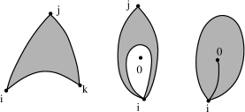
Figure 5. The three types of triangles

The arcs of the triangulation divide the disc into a collection of disjoint triangles. We will often call them the triangles of $\mathcal{T}$. There are three types of triangles appearing, as shown in Figure 5. If the disc has no puncture, the only triangles appearing have three vertices and three arcs as sides. If the disc has a puncture, there are two more types of triangles, one with sides $D_{ij}$, $D_{ji}$ and $D_{ii}$ ($i,j\neq 0$) and one with the corresponding sides obtained by setting $j=0$. The latter is called a self-folded triangle. These three types correspond to the triangles of label A₁, A₂ and A₄ of Burman, cf. [B99] and are called ideal triangles in [FST06] - our notion of triangulation is thus an ideal triangulation in [FST06].

The number of arcs in a triangulation is an invariant of the disc. It is clear that any triangulation of $S$ has $N-3$ arcs and $N-2$ triangles whereas triangulations of punctured discs $S_{\odot}$ have $N$ arcs and $N$ triangles.

We often need to refer to a subset $V_{kl}$ of the vertices of the disc:

Definition 2.3.

For $1\leq k,l\leq N$ we write $V_{kl}:=V(B_{k,l})$ to denote the vertices of the boundary arc $B_{k,l}$. In other words, we are referring to the vertices from $k$ to $l$, going clockwise. In case $k>l$, the set $V_{kl}$ consists of the vertices $k,k+1,\dots,N,1,2,\dots,l$.

We will also need to consider truncations $(S_{ij})_{\odot}$ and $S_{ij}$ of the punctured disc $S_{\odot}$, defined as follows:

Definition 2.4.

Let $j\neq i+1$. Together with $D_{ij}$, the boundary arc $B_{ji}$ forms a (smaller) punctured disc which we denote by $(S_{ij})_{\odot}$. Its vertices are $V_{j,i}$. In particular, $j$ is the clockwise neighbour of $i$ in $(S_{ij})_{\odot}$.

On the other hand, $D_{ij}$ and $B_{ij}$ form an unpunctured disc which we denote by $S_{ij}$. Its vertices are $V_{i,j}$, where $i$ is the clockwise neighbour of $j$ in $S_{ij}$.

In $S_{ij}$ and $(S_{ij})_{\odot}$, some of the triangles of $\mathcal{T}$ may be cut open into several different regions. If $D_{ij}$ is not an arc of the triangulation, then there are triangles of $\mathcal{T}$ which are crossed by $D_{ij}$. If $S_{ij}$ contains two connected components of such a triangle we say that $D_{ij}$ splits the triangle.

Remark 2.5.

If $D_{ij}$ is an arc of the triangulation, it does not cut across any triangles. Hence no split triangles appear and the arcs of $\mathcal{T}$ induce triangulations of $(S_{ij})_{\odot}$ and of $S_{ij}$.

Definition 2.6.

Let $S_{\odot}$ be a punctured disc with triangulation $\mathcal{T}$.
We denote by $\mathcal{T}|_{S_{ij}}$ the subdivision of $S_{ij}$ into triangles and regions obtained from restricting the triangulation $\mathcal{T}$ to $S_{ij}$.
In the same way, $\mathcal{T}|_{(S_{ij})_{\odot}}$ denotes the subdivision of $(S_{ij})_{\odot}$ into triangles and regions obtained from restricting $\mathcal{T}$ to $(S_{ij})_{\odot}$.

(a) no splitting

(b) splitting occurs

Figure 6. Restricted triangulations through truncation by the arc $D_{ij}$

Figure 6 presents two examples, one where no triangles are split and one where $D_{ij}$ splits triangles. Note that by the observations above, $\mathcal{T}|_{S_{ij}}$ and $\mathcal{T}|_{(S_{ij})_{\odot}}$ are triangulations of the corresponding discs if and only if $D_{ij}\in\mathcal{T}$.

Remark 2.7.

Consider the arc $D_{ij}$ (where $j\neq i+1$) in a punctured disc $S_{\odot}$ with triangulation $\mathcal{T}$. If there is a $k$ in $V_{j,i}$ such that $\mathcal{T}$ contains the central arc $D_{k0}$, then $\mathcal{T}|_{S_{ij}}$ does not contain any pair of split triangles.

Given a triangulation of any disc (punctured or unpunctured) we are interested in the ways to allocate triangles to a subset $I$ of the vertices. That is we are interested in matchings between a subset of the vertices and a subset of the triangles. In the case of a truncated version of a disc, we want to allocate triangles and regions of the truncated triangulation to vertices.

Definition 2.8.

Let $S$ and $S_{\odot}$ be discs with vertices $\{1,2,\dots,N\}$, $S_{\odot}$ with puncture $0$. Fix a triangulation $\mathcal{T}$ of the disc, let $I$ be a subset of the vertices $\{1,\dots,N\}$.

(i) A matching (for $S$) between $I$ and $\mathcal{T}$ is a way to allocate to each vertex $i\in I$ a triangle of $\mathcal{T}$ incident with $i$ in such a way that no triangle of $\mathcal{T}$ is allocated to more than one vertex.

(ii) A matching (for $S_{\odot}$) between $I\,\cup\,\{0\}$ and $\mathcal{T}$ is a way to allocate $k+1$ triangles of $\mathcal{T}$ to the vertices of $I$ and to the puncture in the same way as above.

(iii) Given an arc $D_{ij}$ in $S_{\odot}$ let $S_{ij}$ be the truncated disc as in Definition 2.4 and let $I\subset V_{i,j}$ be a subset of the vertices between $i$ and $j$. Then a matching (for $S_{ij}$) between $I$ and $\mathcal{T}|_{S_{ij}}$ is a way to allocate $k=|I|$ triangles or regions of $\mathcal{T}|_{S_{ij}}$ to the vertices of $I$ as above.

Remark 2.9.

Matchings as in Definition 2.8 can regarded as complete matchings for the corresponding bipartite graphs (cf. [G85, 11-1]).

Now if $\mathcal{T}$ is a triangulation of a disc (with or without puncture), we want to refer to the set of all matchings between a subset of the vertices of the disc and the triangles of $\mathcal{T}$:

Definition 2.10.

Let $\mathcal{T}$ be a triangulation of a disc and $I$ be a subset of the vertices $\{1,\dots,N\}$ or of $\{1,\dots,N\}\cup\{0\}$ in case the disc has a puncture. Then we set $\mathcal{M}(I,\mathcal{T})$ to be the set of all matchings between $I$ and $\mathcal{T}$.

Remark 2.11.

Let $S_{\odot}$ be a punctured disc with $N$ marked points on the boundary and a fixed triangulation $\mathcal{T}$, and let $i\in\{1,2,\dots,N\}$. Then we distinguish four cases. They are illustrated on the left hand sides of Figures 7,  8, 9 and  10:

(i) $\mathcal{T}$ contains at least two central arcs and $D_{i0}\notin\mathcal{T}$;

(ii) $\mathcal{T}$ contains at least two central arcs and $D_{i0}$ $\in\mathcal{T}$;

(iii) There is exactly one central arc $D_{k0}$ in the triangulation, $i\neq k$;

(iv) The only central arc of $\mathcal{T}$ is $D_{i0}$.

Figure 7. Type (i), $i=8$

Figure 8. Type (ii), $i=8$

Figure 9. Type (iii), $i=8$

Figure 10. Type (iv), $i=8$

We want to associate certain unpunctured discs $P(i)$ and $Q(i)$ to the vertex $i$, in a similar way as we use an arc $D_{ij}$ to define the truncated discs $S_{ij}$ and $(S_{ij})_{\odot}$ obtained from $S_{\odot}$. Here we use one or two central arcs to cut open $S_{\odot}$.

Definition 2.12.

(i) Let $i$ be a marked point of $S_{\odot}$ and $j,k$ boundary vertices with $i\in V_{kj}$ such that $D_{j0},D_{k0}\in\mathcal{T}$ and such that there is no $l\in V_{kj}$ other than $k$, $j$ with $D_{l0}\in\mathcal{T}$. Then we let $P(i)$ be the unpunctured disc with boundary $B_{kj}\cup D_{j0}\cup D_{k0}$. On the other hand we let $Q(i)$ be the unpunctured disc with boundary $B_{jk}\cup\ D_{k0}\cup\ D_{j0}$. Figure 7 illustrates this.

(ii) Let $i$ be a boundary vertex with $D_{i0}\in\mathcal{T}$ and let $j$ be the nearest clockwise neighbour of $i$ with $D_{j0}\in\mathcal{T}$. Then we let $P(i)$ be the unpunctured disk with boundary $B_{ij}\cup D_{j0}\cup D_{i0}$ and $Q(i)$ be the unpunctured disc with boundary $B_{ji}\cup\ D_{i0}\cup\ D_{j0}$. This is illustrated in Figure 8.

(iii) If the only central arc of $\mathcal{T}$ is $D_{k0}$ then we define $P(i)$ to be the unpunctured disc obtained by cutting up the disc at $k$, with boundary $B_{kk}\cup D_{k0}\cup D_{k0}$. We obtain an additional marked point on the boundary. We denote the anti-clockwise neighbour of $0$ by $k$ and the clockwise neighbour of $0$ by $k^{\prime}$. An example is presented in Figure 9.

(iv) If the only central arc of $\mathcal{T}$ is $D_{i0}$ then we define $P(i)$ to be the unpunctured disc obtained by cutting up the disc at $i$, with boundary $B_{ii}\cup D_{i0}\cup D_{i0}$. As before, we obtain an additional marked point on the boundary. We denote the anti-clockwise neighbour of $0$ by $i$ and the clockwise neighbour of $0$ by $i^{\prime}$. An example is presented in Figure 10.

In other words, in the first case we cut the disc $S_{\odot}$ along two central arcs and $Q(i)$ is the complement to $P(i)$. In the latter case we unfold the disc along the only central arc. In particular, $Q(i)$ is not defined in this case.

Remark 2.13.

The vertex $i$ and the puncture $0$ are neighbours in $P(i)$ if and only if the arc $D_{i0}$ is in the triangulation.

Definition 2.14.

For $P(i)$ and $Q(i)$ as defined above, we let $\mathcal{T}|_{P(i)}$ and $\mathcal{T}|_{Q(i)}$ be the triangulations of $P(i)$ and $Q(i)$ obtained from $\mathcal{T}$ by only considering the triangles in $P(i)$ and in $Q(i)$ respectively. Then $\mathcal{T}|_{P(i)}$ and $\mathcal{T}|_{Q(i)}$ are triangulations of unpunctured discs.

With the notation introduced in Definition 2.10 we can now associate numbers $m_{ij}$ to a disc with a fixed triangulation.

Definition 2.15.

Let $S_{\odot}$ be a punctured disc with vertices $\{1,2,\dots,N\}$ and puncture $0$. Fix a triangulation $\mathcal{T}$ of $S_{\odot}$. Let $i,j\in\{1,\dots,N\}$, $j\neq i,i+1$.

• Let $\mathcal{M}_{ij}:=\mathcal{M}(V_{i+1,j-1},\mathcal{T}|_{S_{ij}})$, i.e. the set of matchings between $V_{i+1,j-1}$ and $\mathcal{T}|_{S_{ij}}$.

• Let $\mathcal{M}_{i0}:=\mathcal{M}(V(P(i)\setminus\{i,0\}),\mathcal{T}\mid_{P(i)})$.

• Let $\mathcal{M}_{ii}:=\mathcal{M}(V_{i+1,i-1}\cup\{0\},\mathcal{T})$.

We set $m_{i,i+1}=1$, $m_{ij}=|\mathcal{M}_{ij}|$, $m_{i0}=|\mathcal{M}_{i0}|$ and $m_{ii}=|\mathcal{M}_{ii}|$.

3. The unpunctured case

In this section we recall the frieze patterns of Conway and Coxeter and describe various interpretations of their entries and properties that they satisfy. We will phrase these results in terms of our set-up above.

In [CoCo73a], [CoCo73b], Conway and Coxeter studied frieze patterns of positive numbers. These are patterns of positive integers arranged in a finite number of rows where the top and bottom rows consist of $1$’s. The entries in the second row appear between the entries in the first row, the entries in the third row appear between the entries in the second row, and so on. Also, for every diamond of the form $\begin{array}[]{rcl}&b\\ a&&d\\ &c\end{array}$ the relation $ad-bc=1$ must be satisfied. The order $N$ of the pattern is one more than the number of rows. For an example see Figure 1.

Conway and Coxeter proved in [CoCo73a, CoCo73b] that the second row of a frieze pattern of order $n$ is equal to the sequence of numbers of triangles at the vertices of a triangulation of a disc with $N$ marked points. Start with a vertex $i$ of $S$ and label it $0$. Whenever $i$ is connected to another vertex $j$ by an edge (including boundary edges) of $\mathcal{T}$, label $j$ by $1$. Furthermore, if $\triangle$ is a triangle with exactly two vertices which have been labelled already, label the third vertex with the sum of the other two labels. Iterating this procedure, we obtain labels for all vertices of $S$. The labels clearly depend on $i$ and the label obtained at $j$ (for $j\neq i$) is denoted by $(i,j)$.

Remark 3.1.

Note that it is clear from the definition that $(i,i+1)=1$ for all $i$ and that $(i,j)=1$ whenever $i$ and $j$ are the two ends of an arc of $\mathcal{T}$.

The frieze pattern corresponding to $\mathcal{T}$ can then be described by displaying the numbers $(i,j)$ in the following way:

$$\begin{array}[]{ccccccccc}(1,2)&&(2,3)&&\cdots&&\cdots&&(N-1,N)\\ &(1,3)&&\cdots&&\cdots&&(N-2,N)&\\ &&\ddots&&&&\iddots&&\\ &&&(1,N-1)&&(2,N)&&&\\ &&&&(1,N)&&&&\end{array}$$

This fundamental region is then repeated upside down to the right and left, then the right way up on each side, and so on. Broline, Crowe and Isaacs have given the following interpretation of the numbers $(i,j)$.

Theorem 3.2.

[BCI74, Theorem 1] Let $S$ be a disc with $N$ marked points on the boundary with triangulation $\mathcal{T}$. Let $i,j$ be distinct marked points. Then:
(a) We have that $(i,j)$ is equal to $|\mathcal{M}(V_{i+1,j-1},\mathcal{T})|$, i.e. the number of matchings between $\mathcal{T}$ and $i+1,\ldots,j-1$.
(b) We have that $(i,j)=|\mathcal{M}(V_{j+1,i-1},\mathcal{T})|$.
In particular, $(i,j)=(j,i)$.

Definition 3.3.

Let $i,j$ be a distinct pair of marked points on the boundary of $S$, and let $\mathcal{T}$ be a triangulation of $S$. Let $n_{ij}=M(\{1,\dots,N\}\setminus\{i,j\},\mathcal{T})$, i.e. the number of matchings between $\{1,2,\dots,N\}\setminus\{i,j\}$ and $\mathcal{T}$.

Carroll and Price have shown that the numbers $(i,j)$ coincide with the $n_{ij}$ defined above. This is discussed in [P05].

Theorem 3.4.

[CaPr03] With the notation above, $(i,j)=n_{ij}$ for any pair of distinct vertices $i,j$.

We shall freely use this result in the sequel, in particular noting that the $n_{ij}$ have the properties of the $(i,j)$ that we have described above.

Propp reports that one of the main steps in the proof of Carroll and Price is the following, which is a direct consequence of the Condensation Lemma of Kuo [K04, Theorem 2.5].

Proposition 3.5.

Let $i,j,k,l$ be four boundary vertices of $S$ in clockwise order around the boundary of $S$. Then:

$$n_{ik}n_{jl}=n_{ij}n_{kl}+n_{li}n_{jk}.$$

Finally, we note that the numbers $(i,j)$ can be interpreted as specialisations of cluster variables by work of Fomin and Zelevinsky [FZ03, 12.2]. Let $\mathcal{A}$ be a cluster algebra of type $A_{N-3}$ with trivial coefficients. Then the cluster variables of $\mathcal{A}$ are in bijection with the set consisting of all of the diagonals of $S$ (using also [FZ01]). For distinct vertices $i,j$, let $x_{ij}$ be the cluster variable corresponding to the diagonal $D_{ij}$ of $S$. By [FZ02, 3.1], $x_{ij}$ is a Laurent polynomial in the cluster variables corresponding to the diagonals of $\mathcal{T}$.

The following result is proved in [P05, §3] (for the $n_{ij}$), but we include a proof for the convenience of the reader. We also note that a connection between frieze patterns and cluster algebras was first explicitly given in [CaCh06].

Theorem 3.6.

Let $i,j$ be distinct vertices on the boundary of $S$. Then $(i,j)$ is equal to the number $u_{ij}$ obtained from $x_{ij}$ by specialising each of the cluster variables corresponding to the arcs of $\mathcal{T}$ to $1$.

Proof.

This follows from [FZ03] together with Theorem 3.4 and Proposition 3.5, which show that the $(i,j)$ and the $u_{ij}$ both satisfy the relations of Proposition 3.5. Since $(i,j)=1$ is equal to the specialisation of $x_{ij}$ whenever $D_{ij}$ is an arc in $\mathcal{T}$, the equality for arbitrary diagonals follows from iterated application of these relations. ∎

4. Construction of frieze patterns of type $D_{N}$

Our aim in this section is to prove the main result, that the numbers $m_{ii}$, $m_{ij}$ and $m_{i0}$ form a frieze pattern of type $D$. In order to do that we have to prove that the frieze relations (see Section 1) hold. We now work with the disc $S_{\odot}$ with puncture $0$ and $N$ marked points on the boundary labelled $\{1,2,\ldots,N\}$. We first need the following result.

Lemma 4.1.

Let $\mathcal{T}$ be a triangulation of $S_{\odot}$, and let $i,j\in\{1,\dots,N\}$ with $j\neq i+1$.

(1) If $D_{ij}\in\mathcal{T}$ then $m_{ij}=1$.

(2) If $D_{i0}\in\mathcal{T}$ then $m_{i0}=1$.

Proof.

(1) Consider the truncated disc $S_{ij}$ with boundary $B_{ij}$ and $D_{ij}$. Since $D_{ij}\in\mathcal{T}$, none of the triangles of $\mathcal{T}$ are split by $D_{ij}$ and $\mathcal{T}|S_{ij}$ is a triangulation of $S_{ij}$. Suppose first that $i\neq j$. Then $m_{ij}$ is the number of matchings between $\{i+1,\dots,j-1\}$ and $\mathcal{T}|_{S_{ij}}$. Such a matching is a matching between $\mathcal{T}|_{S_{ij}}$ and all of the vertices of the unpunctured disc $S_{ij}$ except $i$ and $j$ which are neighbours on the boundary of $S_{ij}$. By Remark 3.1, $m_{ij}=1$.

Suppose instead that $i=j$. Then $m_{ii}$ is the number of matchings between $\{1,2,\ldots,N\}\setminus\{i\}\cup\{0\}$. Such a matching is a matching between $\mathcal{T}|_{S_{ii}}$ and all of the vertices of the unpunctured disc $P(i)$ except $i$ and $i^{\prime}$ which are joined by the arc $D_{ii^{\prime}}$ in $P(i)$ induced by the arc $D_{ii}$ of $\mathcal{T}$. By Remark 3.1, $m_{ii}=1$.

(2) If $D_{i0}\in\mathcal{T}$ then $i$ and $0$ are neighbours in $P(i)$ and the statement follows with the same reasoning. ∎

Remark 4.2.

We recall that in a triangulation of an unpunctured disc with $N$ marked points on the boundary, there are $N-2$ triangles. It follows that there are no matchings between a triangulation of the disc and a subset of the boundary vertices of cardinality greater than $N-2$.

Definition 4.3.

Let $M$ be a matching between a subset $I$ of $\{1,\ldots,N\}\cup\{0\}$ and a triangulation $\mathcal{T}$ of $S_{\odot}$. Let $P$ be a subset of $S_{\odot}$ consisting of a union of triangles of $\mathcal{T}$. We denote by $M|_{P}$ the restriction of $M$ to $P$: this is the matching between $\mathcal{T}|_{P}$ and $I\cap P$ obtained by allocating each vertex its corresponding triangle in $M$ whenever that triangle is contained in $P$.

In order to do some computations of numbers of matchings, we need the following simple observation:

Lemma 4.4.

Let $\mathcal{T}$ be a triangulation of $S_{\odot}$, and let $S_{\odot}=P\cup Q$ be a decomposition of $S_{\odot}$ into two subsets with common boundary given by arcs of $\mathcal{T}$. Given a subset $I$ of $\{1,2,\ldots,N\}\cup\{0\}$, let $J$ denote the subset of $I$ consisting of vertices on the common boundary between $P$ and $Q$. Then the number of matchings between $\mathcal{T}$ and $I$ is given by

$$|\mathcal{M}(I,\mathcal{T})|=\sum_{J^{\prime},J^{\prime\prime}\,:J=J^{\prime}\sqcup J^{\prime\prime}}n_{J^{\prime},J^{\prime\prime}}.$$

Here $n_{J^{\prime},J^{\prime\prime}}$ is the number of matchings between $\mathcal{T}$ and $I$ in which all vertices of $J^{\prime}$ are allocated triangles in $P$ and all vertices of $J^{\prime\prime}$ are allocated triangles in $Q$. It is given by the product of the number of matchings between $\mathcal{T}|_{P}$ and $I\setminus J^{\prime}$ and the number of matchings between $\mathcal{T}|_{Q}$ and $I\setminus J^{\prime\prime}$.

Proof.

Let $M$ be a matching between $I$ and $\mathcal{T}$. Given a pair $M_{P},M_{Q}$ of matchings for $\mathcal{T}|_{P}$ and $\mathcal{T}|_{Q}$ which are compatible in the sense that any vertex of $J$ is allocated precisely one triangle in either $\mathcal{T}|_{P}$ or $\mathcal{T}|_{Q}$ (but not both), we can put them together to obtain a matching $M$ between $I$ and $\mathcal{T}$. This gives us a bijection between matchings $M$ between $I$ and $\mathcal{T}$ and compatible pairs $M^{\prime},M^{\prime\prime}$ of matchings for $\mathcal{T}|_{P}$ and $\mathcal{T}|_{Q}$. The result follows from dividing up such pairs according to the allocation of the vertices of $J$ to triangles in $P$ or in $Q$. ∎

Lemma 4.5.

Let $\mathcal{T}$ be a triangulation of $S_{\odot}$. Let $d_{0}$ denote the number of triangles of $\mathcal{T}$ incident with the puncture, $0$, and let $i$ denote any boundary vertex of $S_{\odot}$. Then we have $d_{0}m_{i0}=m_{ii}$.

Proof.

If there are at least two arcs incident with $0$ in $\mathcal{T}$, let $j$ be the first boundary vertex strictly clockwise from $i$ such that $D_{j0}\in\mathcal{T}$, and let $k$ be the first boundary vertex anticlockwise from $i$ (possibly equal to $i$) such that $D_{k0}\in\mathcal{T}$. Since there are no arcs of the form $D_{l0}\in\mathcal{T}$ for $l\in V_{k+1,j-1}$, we have $D_{kj}\in\mathcal{T}$. If there is only one arc $D_{l0}$ incident with $0$ in $\mathcal{T}$ then we take $j=k=l$. In this case $D_{jj}\in\mathcal{T}$.

If there is more than one arc incident with $0$ in $\mathcal{T}$, then we have a decomposition of the disc $S_{\odot}$ into smaller discs $P(i)$ and $Q(i)$ (Definition 2.12). We shall apply Lemma 4.4 in these cases. For $i,j$ any pair of boundary vertices of $P(i)$, let $p_{ij}$ denote the number of matchings of $\mathcal{T}|_{P(i)}$ with all of the boundary vertices of $P(i)$ except $i$ and $j$. Let $q_{ij}$ denote the corresponding number for a pair of boundary vertices of $Q(i)$.

Case (I): We assume first that $i,j$ and $k$ are all distinct. See Figure 11(a). If, in a matching in $\mathcal{M}_{ii}$, both $j$ and $k$ are allocated triangles in $P(i)$ then $0$ must be allocated a triangle in $Q(i)$ by Remark 4.2 applied to $P(i)$. By restriction of such a matching to $P(i)$ we obtain a matching for $\mathcal{T}|_{P(i)}$ in which $i$ and $0$ are not allocated triangles and by restriction to $Q(i)$ we obtain a matching for $\mathcal{T}|_{Q(i)}$ in which $j$ and $k$ are not allocated triangles. Thus there are $p_{i0}q_{jk}$ matchings in $\mathcal{M}_{ii}$ in which $j$ and $k$ are both allocated triangles in $P(i)$. Using the fact that $p_{i0}=m_{i0}$ (by definition) and Theorem 3.2, we see that this is equal to $m_{i0}(d_{0}-1)$. If $j$ is allocated a triangle in $Q(i)$ and $k$ is allocated a triangle in $P(i)$ then $0$ is allocated a triangle in $P(i)$ by Remark 4.2 applied to $Q(i)$, and we obtain $p_{ij}q_{0k}=p_{ij}\cdot 1=p_{ij}$ matchings of this type by Remark 3.1. Similarly, there are $p_{ij}$ matchings in $\mathcal{M}_{ii}$ in which $j$ is allocated a triangle in $P(i)$ and $k$ is allocated a triangle in $Q(i)$.

There are no matchings in $\mathcal{M}_{ii}$ in which both $j$ and $k$ are both allocated triangles in $Q(i)$, by Remark 4.2 applied to $Q(i)$, so we have covered all cases. By Lemma 4.4 we have that $m_{ii}=|\mathcal{M}_{ii}|=(d_{0}-1)m_{i0}+p_{ij}+p_{ik}$. By Proposition 3.5, $p_{i0}p_{jk}=p_{ij}p_{0k}+p_{ik}p_{0j}$. Since $D_{kj}\in\mathcal{T}$, $p_{jk}=1$ by Remark 3.1, and we also have by Remark 3.1 that $p_{0j}=p_{0k}=1$, so $p_{ij}+p_{ik}=p_{i0}=m_{i0}$. We obtain

$$m_{ii}=(d_{0}-1)m_{i0}+m_{i0}=d_{0}m_{i0}$$

as required.

(a) Case I

(b) Case II

Figure 11. Proof of Lemma 4.5, Cases (I) and (II)

Case (II): We assume next that $i=k$. See Figure 11(b). If, in a matching in $\mathcal{M}_{ii}$, $j$ is allocated a triangle in $P(i)$, then $0$ must be allocated a triangle in $Q(i)$ by Remark 4.2 applied to $P(i)$, and we see that there are $p_{i0}q_{ij}$ matchings of this type. By Theorem 3.2 this is equal to $m_{i0}(d_{0}-1)=d_{0}-1$, noting that $m_{i0}=1$ by Lemma 4.1. If $j$ is allocated a triangle in $Q(i)$, then $0$ must be allocated a triangle in $P(i)$ by Remark 4.2 applied to $Q(i)$. We obtain $p_{ij}q_{0i}=1\cdot 1=1$ matchings of this type by Remark 3.1. By Lemma 4.4 we obtain a total number of matchings $m_{ii}=|\mathcal{M}_{ii}|=d_{0}-1+1=d_{0}=m_{i0}d_{0}$ as required.

Case (III): We assume next that $i\not=j=k$. In a matching in $\mathcal{M}_{ii}$, only one of $j,j^{\prime}$ is allocated a triangle. See Figure 12.

We see that $m_{ii}$ is given by the the sum of the number of matchings between $\mathcal{T}|_{P(i)}$ and $V_{i+1,i-1}\cup\{0\}$ and the number of matchings between $\mathcal{T}|_{P(i)}$ and $V_{i+1,i-1}\cup\{0\}$ with $j$ replaced by $j^{\prime}$. There are $p_{ij}$ matchings of the first kind and $p_{ij^{\prime}}$ matchings of the second kind, making a total of $p_{ij}+p_{ij^{\prime}}$. We have that $p_{i0}p_{jj^{\prime}}=p_{ij}p_{0j}+p_{ij^{\prime}}p_{0j^{\prime}}$, by Proposition 3.5, so $m_{i0}=p_{i0}=p_{ij}+p_{ij^{\prime}}$ by Remark 3.1, noting that $0,j$ and $0,j^{\prime}$ are adjacent on the boundary of $P(i)$ and $D_{j^{\prime}j}$ lies in $\mathcal{T}|_{P(i)}$. We obtain $m_{ii}=m_{i0}=m_{i0}d_{0}$ as required.

Figure 12. Proof of Lemma 4.5, Case (III).

Case (IV) We finally assume that $i=j=k$, so that there is a unique arc incident with $0$ in $\mathcal{T}$ given by $D_{i0}$. See Figure 13. We have that $m_{ii}$ is given by the the number of matchings between $V_{i+1,i-1}\cup\{0\}$ and $\mathcal{T}|_{P(i)}$, so we obtain $m_{ii}=p_{ii^{\prime}}=1$ by Remark 3.1 since $D_{i^{\prime}i}\in\mathcal{T}|_{P(i)}$. Hence $m_{ii}=d_{0}m_{i0}$ as required, since $d_{0}=1$ and $m_{i0}=1$ by Lemma 4.1.

Figure 13. Proof of Lemma 4.5, Case (IV).

The proof of Lemma 4.5 is complete. ∎

In order to prove the frieze relations hold, we first need the following:

Lemma 4.6.

Let $\mathcal{T}$ be a triangulation of $S_{\odot}$. Let $i,j$ be boundary vertices of $S_{\odot}$ with $j\neq i+1$. Then the restriction $\mathcal{T}|_{S_{ij}}$ can be extended to a triangulation of the entire disc $S$ with different marked points and the puncture removed.

Proof.

Let $a_{1},a_{2},\ldots,a_{t}$ be the vertices on the arc $B_{i,j}$ (distinct from $i$ and $j$) in order clockwise from $i$, which lie on arcs of $\mathcal{T}$ whose other end lies in $V_{j+1,i-1}$ For each $l$, let $b_{l,1},b_{l,2},\ldots,b_{l,u_{l}}$ be the end-points (other than $a_{l}$) of the arcs of $\mathcal{T}$ incident with $a_{l}$ whose other end lies in $V_{j+1,i-1}$.

The arc $D_{i,a_{1}}$ must lie in $\mathcal{T}$, else the region on the $i$-side of the arc $D_{a_{1},b_{l,1}}$ will not be a triangle, since the other end-point of any arc incident with any of the vertices on the boundary arc $B_{i+1,a_{1}-1}$ can only be a vertex on the boundary arc $B_{i,a_{1}}$. Similarly, the arcs $D_{a_{m},a_{m+1}}$ must all be in $\mathcal{T}$, as must $D_{a_{t},j}$.

Remove the vertices $V_{j+1,i-1}$ and introduce new vertices on the boundary between $j$ and $i$ labelled

$$c_{1,1},c_{1,2},\ldots,c_{1,u_{1}},c_{2,1},\ldots,c_{l,u_{l}},$$

going anticlockwise from $i$ to $j$. We identify $c_{m,u_{m}}$ with $c_{m+1,1}$ for each $m$. We replace the part of each arc $D_{a_{m},b_{l,m}}$ below the arc $D_{i,j}$ with a new arc linking $c_{l,m}$ with the intersection of $D_{a_{m},b_{l,m}}$ and $D_{i,j}$, and add arcs $D_{c_{1,1},i}$ and $D_{j,c_{t,u_{t}}}$. See Figure 14 for an example. In this way we can complete $\mathcal{T}|_{S_{i,j}}$ to a triangulation of the disc $S$, with new marked points on the boundary and the puncture removed, as required. ∎

Figure 14. Completing to a triangulation of the unpunctured disc.

We first note the following consequence:

Lemma 4.7.

Let $\mathcal{T}$ be a triangulation of $S_{\odot}$. Let $i,j$ be boundary vertices of $S_{\odot}$ with $j\neq i,i+1$. Then the numbers $m_{ii}$, $m_{ij}$ and $m_{i0}$ as in Definition 2.15 are all positive.

Proof.

By Definition 2.15, the $m_{i0}$ can be interpreted as entries in Conway-Coxeter frieze patterns (using Theorem 3.4), so are positive. By Lemma 4.6 the same argument applies to the $m_{ij}$. Then the $m_{ii}$ are positive by Lemma 4.5. ∎

We can now prove that the frieze relations hold:

Proposition 4.8.

Let $\mathcal{T}$ be a triangulation of $S_{\odot}$. Let $i,j$ be boundary vertices of $S_{\odot}$ with $j\neq i,i+1$, Let the numbers $m_{ii}$, $m_{ij}$ and $m_{i0}$ be as in Definition 2.15. Then the following hold:

(5) $$m_{ij}\cdot m_{i+1,j+1} = m_{i+1,j}\cdot m_{i,j+1}+1,\mbox{ provided $j\not=i$ or $i+1$}$$

(6) $$m_{i,i-1}\cdot m_{i+1,i} = m_{i+1,i-1}\cdot m_{ii}\cdot m_{i0}+1$$

(7) $$m_{ii}\cdot m_{i+1,0} = m_{i+1,i}+1$$

(8) $$m_{i0}\cdot m_{i+1,i+1} = m_{i+1,i}+1$$

Proof.

We prove each relation in turn.
Proof of (1): By Lemma 4.6 we can complete $\mathcal{T}|_{S_{i,j+1}}$ to a triangulation $\mathcal{T}^{\prime}$ of the disc $S$ (with the puncture removed) and new marked points on the boundary. We see that $m_{i,j+1}$ is the number of matchings between $\mathcal{T}^{\prime}$ and $V_{i+1,j-1}$. It is clear that $m_{ij}$, $m_{i+1,j}$ and $m_{i,j+1}$ are the numbers of matchings between $\mathcal{T}^{\prime}$ and $V_{i+1,j-1}$, $V_{i+2,j-1}$ and $V_{i+1,j}$ respectively. Hence the frieze relation (1) holds by Proposition 3.5.

Proof of (2): We adopt the same notation for $j$ and $k$ as in the proof of Lemma 4.5.

Let $\widetilde{\mathcal{M}}_{ii}$ denote the set of matchings between $I:=\{1,2,\ldots,N\}\setminus\{i\}$ and $\mathcal{T}|_{S_{ii}}$. Set $\widetilde{m}_{ii}=|\widetilde{\mathcal{M}}_{ii}|$. It is straightforward to show (along the lines of the proof of (1)) that, for any boundary vertex $i$ of $S_{\odot}$,

$$m_{i,i-1}m_{i+1,i}=m_{i+1,i-1}\widetilde{m}_{ii}+1.$$

Hence for (2) it is enough to show that $\widetilde{m}_{ii}=m_{i0}m_{ii}$. By Lemma 4.5, this is equivalent to showing that $\widetilde{m}_{ii}=d_{0}m_{i0}^{2}$.

If there is more than one arc incident with $0$ in $\mathcal{T}$, then we have a decomposition of the disc $S_{\odot}$ into smaller discs $P(i)$ and $Q(i)$ (see Definition 2.12). We shall apply Lemma 4.4 in these cases. Let $p_{ij}$ and $q_{ij}$ be as in Lemma 4.5.

Proof of (2), Case (I): We assume first that $i,j$ and $k$ are distinct. See Figure 15(a).

(a) Case I

(b) Case II

Figure 15. Proof of Proposition 4.8(2), Cases (I) and (II)

(a) Suppose first that in a matching in $\widetilde{\mathcal{M}}_{ii}$, $j,k$ are both allocated triangles in $P(i)$. Then restricting the matching to $P(i)$ we obtain a matching between $\mathcal{T}|_{S_{ii}}$ and $V_{i+1,j}\cup V_{k,i-1}$. Since the arc $D_{ii}$ splits $P(i)$ completely, there are $|\mathcal{M}(V_{i+1,j},\mathcal{T}|_{P(i)})|\cdot|\mathcal{M}(V_{k,i-1},\mathcal{T}|_{P(i)})|$ of these. By Theorem 3.2, this is equal to $m_{i0}^{2}$. Restricting $\mathcal{T}$ to $Q(i)$, no triangles are split by $D_{ii}$. Therefore there are $|\mathcal{M}(V_{j+1,k-1},\mathcal{T}|_{Q(i)})|$ matchings of this type in $\widetilde{\mathcal{M}}_{i}i$. By Theorem 3.2, this is equal to $\mathcal{M}(\{0\},\mathcal{T}|_{Q(i)})=d_{0}-1$. We see that there are $(d_{0}-1)m_{i0}^{2}$ matchings in $\widetilde{\mathcal{M}}_{ii}$ in which $j$ and $k$ are both allocated triangles in $P(i)$.

(b) Arguing as above we see that there are $|\mathcal{M}(V_{k+1,i-1},\mathcal{T}|_{P(i)})|\cdot|\mathcal{M}(V_{i+1,j},\mathcal{T}|_{P(i)})|$ possible restrictions to $P(i)$ of a matching in $\widetilde{\mathcal{M}}_{ii}$ in which $j$ is allocated a triangle in $P(i)$ and $k$ a triangle in $Q(i)$. By Theorem 3.2 this is equal to $p_{ki}p_{i0}=p_{ki}m_{i0}$. Similarly we see that there are $|\mathcal{M}(V_{j+1,k},\mathcal{T}|_{Q(i)})|=q_{j0}=1$ possible restrictions to $Q(i)$, the last equality using Remark 3.1. We get a total of $p_{ki}m_{i0}$ matchings of this type in $\widetilde{\mathcal{M}}_{ii}$.

(c) Arguing as in (b) we see that there are $p_{ji}m_{i0}$ matchings in $\widetilde{\mathcal{M}}_{ii}$ in which $j$ is allocated a triangle in $Q(i)$ and $k$ a triangle in $P(i)$.

(d) By Remark 4.2 for $Q(i)$, $j$ and $k$ cannot both be allocated triangles in $Q(i)$ for any matching in $\widetilde{\mathcal{M}}_{ii}$.

By Lemma 4.4 we see that $\widetilde{m}_{ii}=(d_{0}-1)m_{i0}^{2}+(p_{ki}+p_{ij})p_{i0}$. But by Proposition 3.5, $p_{i0}=p_{ij}+p_{ki}$, so $\widetilde{m}_{ii}=d_{0}m_{i0}^{2}$ as required.

Proof of (2), Case (II): We next assume that $i=k\not=j$. See Figure 15(b).

(a) There are $|\mathcal{M}(V_{i+1,j},\mathcal{T}|_{P(i)})|$ possible restrictions to $P(i)$ of a matching in $\widetilde{\mathcal{M}}_{ii}$ in which $j$ is allocated a vertex in $P(i)$. There are $|\mathcal{M}(V_{j+1,i-1},\mathcal{T}|_{Q(i)})|$ possible restrictions to $Q(i)$, giving a total of

$$|\mathcal{M}(V_{i+1,j},\mathcal{T}|_{P(i)})|\cdot|\mathcal{M}(V_{j+1,i-1},\mathcal{T}|_{Q(i)})|=p_{i0}|\mathcal{M}(\{0\},\mathcal{T}|_{Q(i)})|=(d_{0}-1)$$

by Theorem 3.2 and the fact that $p_{i0}=m_{i0}=1$ (by Lemma 4.1).

(b)There are $|\mathcal{M}(V_{i+1,j-1},\mathcal{T}|_{P(i)})|$ possible restrictions to $P(i)$ of a matching in $\widetilde{\mathcal{M}}_{ii}$ in which $j$ is allocated a triangle in $Q(i)$. There are $|\mathcal{M}(V_{j,i-1},\mathcal{T}|_{Q(i)})|$ possible restrictions to $Q(i)$. By Theorem 3.2 this is equal to $p_{ij}q_{i0}$, which is equal to $1$ by Lemma 4.1.

By Lemma 4.4, we have $\widetilde{m}_{ii}=d_{0}-1+1=d_{0}$. This equals $m_{i0}d_{0}$ by Lemma 4.1 so we are done.

Proof of (2), Case (III): We next assume that $j=k\not=i$. See Figure 16.

Figure 16. Proof of Proposition 4.8(2), Case (III).

A matching in $\widetilde{\mathcal{M}}_{ii}$ induces a matching of $\mathcal{T}|_{P(i)}$ in which either $j$ or $j^{\prime}$ is allocated a triangle but not both. Since $P(i)$ is split by $D_{ii}$ completely, there are $|\mathcal{M}(V_{j^{\prime},i-1},\mathcal{T}|_{P(i)})|\cdot|\mathcal{M}(V_{i+1,j-1},\mathcal{T}|_{P(i)})|$ matchings of the first kind. By Theorem 3.2 this is equal to $p_{i0}p_{ij}$. Similarly there are $p_{ij^{\prime}}p_{i0}$ matchings of the second kind.

We get a total of $p_{i0}(p_{ij}+p_{ij^{\prime}})$ matchings in $\widetilde{\mathcal{M}}_{ii}$. By Proposition 3.5 we see that $p_{i0}=p_{ij}+p_{ij^{\prime}}$, and we obtain $\widetilde{m}_{ii}=p_{i0}^{2}=m_{i0}^{2}=d_{0}m_{i0}^{2}$ as required, since $d_{0}=1$.

Proof of (2), Case (IV): Finally we consider the case where $i=j=k$. See Figure 17.

Figure 17. Proof of Proposition 4.8(2), Case (IV).

A matching in $\widetilde{\mathcal{M}}_{ii}$ induces a matching of $\mathcal{T}|_{P(i)}$ in which all boundary vertices except $i$ and $i^{\prime}$ are allocated a triangle. Since $D_{i^{\prime}i}$ is an arc in $\mathcal{T}|_{P(i)}$, we see by Remark 3.1 that there is only one possible such matching. So $\widetilde{m}_{ii}=1=d_{0}m_{i0}$, since $m_{i0}=1$ by Lemma 4.1.

Proof of (3): We note that by Lemma 4.5, it is sufficient to show that $d_{0}m_{i0}m_{i+1,0}=m_{i+1,i}+1$.

Proof of (3), Case (I): We first assume that $i,i+1,j$ and $k$ are all distinct. See Figure 18(a).

(a) Case I

(b) Case II

Figure 18. Proof of Proposition 4.8(3), Cases (I) and (II)

(a) There are $|\mathcal{M}(V_{i+2,j},\mathcal{T}|_{P(i)})|\cdot|\mathcal{M}(V_{k,i-1},\mathcal{T}|_{P(i)})|$ possible restrictions to $P(i)$ of a matching in $\mathcal{M}_{i+1,i}$ in which both $j$ and $k$ are allocated triangles in $P(i)$, since $D_{i+1,i}$ splits $P(i)$ completely. By Theorem 3.2 (and the definition of $m_{i0}$ and $m_{i+1,0}$), this equals $m_{i+1,0}m_{i0}$. There are $|M(V_{j+1,k-1},\mathcal{T}|_{Q(i)})|$ possible restrictions to $Q(i)$, which by Theorem 3.2 is equal to $|M(\{0\},\mathcal{T}|_{Q(i)})|=d_{0}-1$. Hence there are $(d_{0}-1)m_{i0}m_{i+1,0}$ matchings in $\mathcal{M}_{i+1,i}$ in total in which both $j$ and $k$ are allocated triangles in $P(i)$.

(b) There are $|\mathcal{M}(V_{i+2,j},\mathcal{T}|_{P(i)})|\cdot|\mathcal{M}(V_{k+1,i-1},\mathcal{T}|_{P(i)})|$ possible restrictions to $P(i)$ of a matching in $\mathcal{M}_{i+1,i}$ in which $j$ is allocated a triangle in $P(i)$ and $k$ is allocated a triangle in $Q(i)$. By Theorem 3.2 this is equal to $p_{i+1,0}p_{ik}=m_{i+1,0}p_{ik}$. There are $|M(V_{j+1,k},\mathcal{T}|_{Q(i)})|$ possible restrictions to $Q(i)$, which is equal to $q_{0j}$ by Theorem 3.2 and thus equal to $1$ by Remark 3.1. Thus we see that there are a total of $p_{ik}m_{i+1,0}$ matchings in $\mathcal{M}_{i+1,i}$ in which $j$ is allocated a triangle in $P(i)$ and $k$ is allocated a triangle in $Q(i)$.

(c) Arguing in a similar way to (b) we see that there are $p_{i+1,j}m_{i0}$ matchings in $\mathcal{M}_{i+1,i}$ in which $j$ is allocated a triangle in $Q(i)$ and $k$ is allocated a triangle in $P(i)$.

(d) We note that it is not possible for both $j$ and $k$ to be allocated triangles in $Q(i)$ in a matching in $\mathcal{M}_{i+1,i}$, by Remark 4.2 applied to $Q(i)$.

By Lemma 4.4 we see that

$$m_{i+1,i}=(d_{0}-1)m_{i0}m_{i+1,0}+p_{ik}m_{i+1,0}+p_{i+1,j}m_{i0}.$$

By Proposition 3.5 we have that $p_{i0}p_{jk}=p_{ij}p_{0k}+p_{ik}p_{0j}$, so $p_{i0}=p_{ij}+p_{ik}$, noting that $D_{kj}$ is an arc in $\mathcal{T}|_{P(i)}$, so $p_{jk}=1$. Hence

$$m_{i+1,i} = (d_{0}-1)m_{i0}m_{i+1,0}+m_{i+1,0}(p_{i0}-p_{ij})+m_{i0}p_{i+1,j}$$

$$= (d_{0}-1)m_{i0}m_{i+1,0}+m_{i+1,0}(m_{i0}-p_{ij})+m_{i0}p_{i+1,j}$$

$$= (d_{0}-1)m_{i0}m_{i+1,0}+m_{i0}m_{i+1,0}-m_{i+1,0}p_{ij}+m_{i0}p_{i+1,j}$$

$$= (d_{0}-1)m_{i0}m_{i+1,0}+m_{i0}m_{i+1,0}-1$$

$$= d_{0}m_{i0}m_{i+1,0}-1,$$

using the fact that

$$p_{i+1,0}p_{ij} = p_{i+1,j}p_{i0}+p_{0j}p_{i,i+1}$$

$$= p_{i0}p_{i+1,j}+1,$$

from Proposition 3.5. Hence $d_{0}m_{i0}m_{i+1,0}=m_{i+1,i}+1$ as required.

Proof of (3), Case (II): We next assume that $i,i+1$ and $k$ are distinct while $i+1=j$. See Figure 18(b).

(a) There are $|\mathcal{M}(\{0\}\cup V_{k,i-1},\mathcal{T}|_{P(i)})|$ possible restrictions to $P(i)$ of a matching in $\mathcal{M}_{i+1,i}$ in which $k$ is allocated a triangle in $P(i)$. By Theorem 3.2 this is equal to $p_{i0}=m_{i0}$. There are $|\mathcal{M}(V_{i+2,k-1},\mathcal{T}|_{Q(i)})|$ possible restrictions to $Q(i)$, which by Theorem 3.2 is equal to $|\mathcal{M}(\{0\},\mathcal{T}|_{Q(i)})|=d_{0}-1$. We see that there are $(d_{0}-1)m_{i0}$ matchings in $\mathcal{M}_{i+1,i}$ in which $k$ is allocated a triangle in $P(i)$.

(b) There are $|\mathcal{M}(V_{k+1,i-1},\mathcal{T}|_{P(i)})|$ possible restrictions to $P(i)$ of a matching in $\mathcal{M}_{i+1,i}$ in which $k$ is allocated a triangle in $Q(i)$. By Theorem 3.2 this is equal to $p_{ki}$. There are $|\mathcal{M}(V_{i+2,k},\mathcal{T}|_{Q(i)})|$ possible restrictions to $Q(i)$, which by Theorem 3.2 is equal to $q_{0,i+1}$. This equals $1$ by Remark 3.1. We see that there are $p_{ki}$ matchings in $\mathcal{M}_{i+1,i}$ in which $k$ is allocated a triangle in $Q(i)$.

By Lemma 4.4 we obtain $m_{i+1,i}=(d_{0}-1)m_{i0}+p_{ki}.$ But by Proposition 3.5, we have that $p_{i0}=p_{ki}+1$ (using the fact that $D_{i+1,k}$ is an arc in $\mathcal{T}|_{P(i)}$ and Remark 3.1), so we get that $m_{i+1,i}=d_{0}m_{i0}-1$, so $m_{i+1,i}+1=d_{0}m_{i0}m_{i+1,0}$ as required, since $m_{i+1,0}=1$ by Lemma 4.1.

Proof of (3), Case (III): We next assume that $i,i+1$ and $j$ are distinct while $i=k$. See Figure 19(a).

(a) Case III

(b) Case IV

Figure 19. Proof of Proposition 4.8(3), Cases (III) and (IV)

It follows from symmetry with Case (II) above that $d_{0}m_{i+1,0}=m_{i+1,i}+1$, so $d_{0}m_{i+1,0}m_{i0}=m_{i+1,i}+1$ as required, since $m_{i0}=1$ by Lemma 4.1.

Proof of (3), Case (IV): We next assume that $i=j$ and $i+1=k$. See Figure 19(b).

A matching in $\mathcal{M}_{i+1,i}$ is determined by its restriction to $Q(i)$. The number of possible restrictions is $|\mathcal{M}(V_{i+2,i-1},\mathcal{T}|_{Q(i)})|$ which is $|\mathcal{M}(\{0\},\mathcal{T}|_{Q(i)})|=d_{0}-1$ by Theorem 3.2. So $m_{i+1,i}=d_{0}-1$. Since $m_{i0}=m_{i+1,0}=1$ by Lemma 4.1 we obtain $m_{i+1,i}+1=d_{0}m_{i0}m_{i+1,0}$ as required.

Proof of (3), Case (V): We next assume that $i,i+1$ and $j$ are distinct, with $j=k$. See Figure 20.

Figure 20. Proof of Proposition 4.8(3), Case (V).

There are $|\mathcal{M}(V_{i+2,j},\mathcal{T}|_{P(i)})|\cdot|\mathcal{M}(V_{j+1,i-1},\mathcal{T}|_{P(i)})|$ possible restrictions to $P(i)$ of a matching in $\mathcal{M}_{i+1,i}$ in which $j$ gets allocated a triangle, since $D_{i+1,i}$ splits $P(i)$ completely. There are $|\mathcal{M}(V_{i+2,j-1},\mathcal{T}|_{P(i)})|\cdot|\mathcal{M}(V_{j^{\prime},i-1},\mathcal{T}|_{P(i)})|$ possible restrictions to $P(i)$ in which $j^{\prime}$ gets allocated a triangle. Thus the total number of matchings in $\mathcal{M}_{i+1,i}$ is the sum of these, which by Theorem 3.2 is equal to $p_{i+1,0}p_{j^{\prime}i}+p_{i+1,j}p_{0i}$. By Proposition 3.5, $p_{i0}p_{jj^{\prime}}=p_{ij}p_{0j^{\prime}}+p_{ij^{\prime}}p_{0j}$, so $p_{i0}=p_{ij}+p_{ij^{\prime}}$. We thus have that

$$m_{i+1,i} = m_{i+1,0}(p_{i0}-p_{ij})+m_{i0}p_{i+1,j}$$

$$= m_{i+1,0}m_{i0}-m_{i+1,0}p_{ij}+m_{i0}p_{i+1,j}$$

$$= m_{i+1,0}m_{i0}-1$$

$$= d_{0}m_{i0}m_{i+1,0}-1,$$

as required. Here we use the fact that

$$p_{i+1,0}p_{ij}=p_{i+1,j}p_{i0}+p_{0j}p_{i,i+1}=p_{i0}p_{i+1,j}+1$$

from Theorem 3.2 and Remark 3.1, and the fact that $d_{0}=1$.

Proof of (3), Case (VI): We finally assume that $i=j=k$. See Figure 21.

Figure 21. Proof of Proposition 4.8(3), Case (VI).

Since a matching in $\mathcal{M}_{i+1,i}$ is determined its restriction to $P(i)$, which is a matching between $\mathcal{T}|_{P(i)}$ and $V_{i+2,\ldots,i-1}$ we have that $m_{i+1,i}=|\mathcal{M}(V_{i+2,i-1},\mathcal{T}|_{P(i)})$ which equals $p_{i+1,i}$ by Theorem 3.2. By Proposition 3.5, we have that

$$p_{i+1,0}p_{i^{\prime}i}=p_{i+1,i}p_{0i^{\prime}}+p_{i^{\prime},i+1}p_{i0},$$

so, since $m_{i+1,0}=p_{i+1,0}$ (by definition of $m_{i+1,0}$) and $p_{i^{\prime}i}=p_{0i^{\prime}}=p_{i0}=1$ (using Remark 3.1), we obtain $m_{i+1,0}=m_{i+1,i}+1$, so $d_{0}m_{i0}m_{i+1,0}=m_{i+1,i}+1$, as required, since $d_{0}=m_{i0}=1$.

Proof of (4): We note that $m_{i0}m_{i+1,i+1}=m_{i0}d_{0}m_{i+1,0}=m_{ii}m_{i+1,0}$ by Lemma 4.5, so (4) follows from (3).

The proposition is proved. ∎

Theorem 4.9.

Let $\mathcal{T}$ be a triangulation of $S_{\odot}$. Then the numbers $m_{ij}$, $m_{ii}$ and $m_{i0}$ in Definition 2.15 (arranged as in the introduction) form a frieze pattern of type $D_{N}$.

Proof.

This follows immediately from Proposition 4.8 and Lemma 4.7. ∎

5. Tagged triangulations

In Section 4, we have established a way to obtain a frieze pattern of type $D_{N}$ from a triangulation of a punctured disc with $N$ boundary vertices using the matching numbers. Here, we will show that there exist frieze patterns (of type $D_{N}$) which cannot be obtained in the same way. We will describe another way to construct such frieze patterns and will show how they can be associated to tagged triangulations (as defined below).

Definition 5.1.

We denote the frieze pattern of type $D_{N}$ associated in Theorem 4.9 to the triangulation $\mathcal{T}$ of a punctured disc by $F(\mathcal{T})$.

The frieze patterns of the form $F(\mathcal{T})$ do not give all possible frieze patterns of type $D_{N}$, as we will see now.

Definition 5.2.

Let $P$ be a frieze pattern of type $D_{N}$. We define $\iota(P)$ to be the pattern obtained from $P$ by interchanging the last two rows.

Thus, if $\mathcal{T}$ is a triangulation of $S_{\odot}$, $\iota(F(\mathcal{T}))$ is also a frieze pattern of type $D_{N}$. If a triangulation has only one triangle at the puncture (i.e. $d_{0}=1$), then $m_{ii}=m_{i0}$ for all $i$ (by Lemma 4.5), so the process of interchanging the last two rows does not give a new pattern, so $\iota(F(\mathcal{T}))=F(\mathcal{T})$. We claim that in general, $\iota(F(\mathcal{T}))$ cannot be obtained via a triangulation of a punctured disc:

Remark 5.3.

Let $\mathcal{T}$ be a triangulation of a punctured disc $S_{\odot}$. If $\mathcal{T}$ has at least two central arcs then there is no triangulation $\mathcal{T}^{\prime}$ of $S_{\odot}$ such that $\iota(F(\mathcal{T}))=F(\mathcal{T}^{\prime})$.

Proof.

Let $F(\mathcal{T})$ be obtained from the matching numbers $m_{ij}$ of $\mathcal{T}$ and let $\iota(F(\mathcal{T}))$ be defined as above. Assume that $d_{0}>1$. Then since $m_{i0}=d_{0}m_{ii}$ (Lemma 4.5) we have $m_{i0}<m_{ii}$. Now if there exists a triangulation $\mathcal{T}^{\prime}$ of $S_{\odot}$ with matching numbers $m^{\prime}_{ij}$ giving rise to $\iota(F(\mathcal{T}))$, then by Lemma 4.5 (applied to $\mathcal{T}^{\prime}$), the matching numbers of $\mathcal{T}^{\prime}$ must satisfy $m^{\prime}_{i0}<m^{\prime}_{ii}$ for all $i$. But by construction, $m^{\prime}_{i0}=m_{ii}>m_{i0}=m_{ii}^{\prime}$. ∎

We thus have a way to construct a second frieze pattern for every triangulation with $d_{0}>1$. We now recall the definition of tagged arcs resp. of tagged edges as introduced in [FST06, Definition 7.1] for triangulated surfaces and in  [S06, Section 2.1] for punctured polygons respectively. The idea is to attach labels to arcs in the punctured disc $S_{\odot}$:

Definition 5.4.

Let $S_{\odot}$ be a punctured disc with $N$ boundary vertices with puncture $0$. The set of tagged arcs of $S_{\odot}$ is the following:

$$\{D_{ij}^{1},\ D_{i0}^{1},\ D_{i0}^{-1}\mid 1\leq i,j\leq N,\ j\neq i,i+1\}.$$

We will often just write $D_{ij}$ instead of $D_{ij}^{1}$. When drawing tagged arcs, we indicate the label $-1$ of an arc by a short crossing line on it. Arcs labelled $1$ are drawn as the usual arcs, cf. Figure 22.

Remark 5.5.

Note that the tagged arcs are in bijection with the arcs in the sense of Definition 2.1: The arcs $D_{ij}^{1}$ ($j\neq i,i+1$) correspond to the usual arcs $D_{ij}$ ($j\neq i,i+1$), the central arcs $D_{i0}^{1}$ to the usual central arcs $D_{i0}$ and the arcs $D_{i0}^{-1}$ of label $-1$ correspond to the loops $D_{ii}$.

Figure 22. Three tagged triangulations

Following [FST06, Definition 7.7] and [S06, Section 2.4] we can now define tagged triangulations of punctured discs.

Definition 5.6.

A tagged triangulation $\widetilde{\mathcal{T}}$ of $S_{\odot}$ is a collection of tagged arcs of $S_{\odot}$ obtained from a triangulation $\mathcal{T}$ of $S_{\odot}$ as follows:

(i)	If $d_{0}=1$, replace the pair $D_{ii}$, $D_{i0}$ by the tagged arcs $D_{i0}^{-1}$, $D_{i0}^{1}$
	and replace the arcs $D_{ij}$ by tagged arcs $D_{ij}^{1}$.
(ii)	If $d_{0}=k\geq 2$, replace all central arcs $D_{i_{j},0}$ either by $k$ tagged arcs $D_{i_{j},0}^{1}$
	or by $k$ tagged arcs $D_{i_{j},0}^{-1}$.

See Figure 22 for three tagged triangulations for a punctured disc with $5$ boundary vertices.

In other words: if $\mathcal{T}$ is a triangulation of $S_{\odot}$ containing a unique central arc $D_{i0}$ and hence also the loop $D_{ii}$ (in particular, $d_{0}=1$), then $\mathcal{T}$ gives rise to a tagged triangulation $\widetilde{\mathcal{T}}$ whose only central tagged arcs are $D_{i0}^{1}$ and $D_{i0}^{-1}$. If $\mathcal{T}$ has central arcs $D_{i_{1},0},\dots,D_{i_{k},0}$, $k\geq 2$ (so $d_{0}=k\geq 2$), then $\mathcal{T}$ gives rise to two tagged arc triangulations: one with $k$ central tagged arcs $D_{i_{j},0}^{1}$ and one with $k$ central tagged arcs $D_{i_{j},0}^{-1}$.

Definition 5.7.

Let $\widetilde{\mathcal{T}}$ be an arbitrary tagged triangulation of a punctured disc $S_{\odot}$. Then we associate a frieze pattern $F(\widetilde{\mathcal{T}})$ to it as follows:

(a) If $\widetilde{\mathcal{T}}$ has only arcs labelled $1$, let $\mathcal{T}$ be the triangulation of $S_{\odot}$ obtained via the bijection of Remark 5.5. We then define $F(\widetilde{\mathcal{T}})$ as the frieze pattern of the matching numbers of $\mathcal{T}$, i.e. we set $F(\widetilde{\mathcal{T}})=F(\mathcal{T})$.

(b) If $\widetilde{\mathcal{T}}$ has exactly one tagged arc labelled $-1$, say $D_{i0}^{-1}$ and hence also $D_{i0}^{1}$, then let $\mathcal{T}$ be the triangulation of $S_{\odot}$ obtained through the bijection in Remark 5.5. As in (a), we let $F(\widetilde{\mathcal{T}})$ be the frieze pattern $F(\mathcal{T})$ containing the matching numbers of $\mathcal{T}$.

(c) Suppose that $\widetilde{\mathcal{T}}$ has at least two arcs labelled $-1$. Then every arc incident with $0$ must be labelled $-1$. Let $\mathcal{T}^{\prime}$ be the triangulation of $S_{\odot}$ consisting of all arcs $D_{i0}$ such that $D_{i0}^{-1}$ lies in $\widetilde{\mathcal{T}}$ and all arcs $D_{ij}$ (for $i$ and $j$ boundary vertices of $S_{\odot}$) such that $D_{ij}^{1}$ lies in $\widetilde{\mathcal{T}}$. Then we set $F(\widetilde{\mathcal{T}})=\iota(F(\mathcal{T}^{\prime}))$.

We also note the following:

Proposition 5.8.

The entries in a frieze pattern $M$ of type $D_{N}$ associated to a tagged triangulation $\widetilde{\mathcal{T}}$ of a punctured disc are determined by the numbers of triangles incident with the marked points, together with the number of triangles incident with the puncture.

Proof.

Suppose first that $\mathcal{T}$ is a triangulation (without tags). We remark that it follows from the definition of $F(\mathcal{T})$ that an entry $m_{i,i+2}$ in the first row (with $1\leq i\leq N$) is equal to the number of triangles incident with vertex $i$ in $\mathcal{T}$.

It is clear that, by induction on the rows, these entries determine the entries $m_{ij}$ in the pattern for all boundary vertices $i,j$ with $i\not=j$, via relation (5) in Proposition 4.8. Relations (6) and (7) can be used to determine $m_{ii}m_{i0}$ for each boundary vertex $i$. Using Lemma 4.5 we see that all entries in $F(\mathcal{T})$ are determined in cases (a) and (b) of Definition 5.7. In case (c) we have $F(\widetilde{\mathcal{T}})=\iota(F(\mathcal{T}))$ and it is clear that the same approach works for such $\widetilde{\mathcal{T}}$. ∎

6. Cluster algebras and frieze patterns of type $D_{N}$

Let $\mathcal{A}$ be a cluster algebra [FZ02] of type $D_{N}$, as in the classification of cluster algebras of finite type [FZ03]. We consider the case in which all coefficients are set to $1$. The algebra $\mathcal{A}$ is a subring of the rational function field $\mathbb{F}:=\mathbb{Q}(x_{1},x_{2},\ldots,x_{N})$. It is determined by an initial seed, i.e. a pair consisting of a transcendence basis $\mathbf{x}_{0}$ of $\mathbb{F}$ over $\mathbb{Q}$ and a skew-symmetric integer matrix $B_{0}$ with rows and columns indexed by $\mathbf{x}_{0}$. For each element of $\mathbf{x}_{0}$, a new seed can be produced from $(\mathbf{x}_{0},B_{0})$ by a combinatorial process known as mutation. We obtain a collection of seeds via arbitrary iterative mutation of $(\mathbf{x}_{0},B_{0})$.

The transcendence bases arising are known as a clusters and $\mathcal{A}$ is generated by their union. The generators are known as cluster variables. We note that a skew-symmetric matrix $B$ appearing in a seed $(\mathbf{x},B)$ can be encoded by a quiver, with vertices indexed by $\mathbf{x}$ and $b_{xy}$ arrows from the vertex indexed by $x$ to the vertex indexed by $y$ whenever $b_{xy}>0$.

By [FST06, 7.11] (see also [S06]), the cluster variables of $\mathcal{A}$ are in bijection with the set of all tagged arcs in $S_{\odot}$, and the seeds of $\mathcal{A}$ are in bijection with the tagged triangulations of $S_{\odot}$. The matrix $B$ of a seed corresponding to a given tagged triangulation is described in [FST06, 9.6].

Combining the above bijection between cluster variables and tagged arcs with the bijection in Remark 5.5, we obtain a bijection between cluster variables and the arcs of $S_{\odot}$ in the sense of Definition 2.1. For $D_{ij}$ (respectively, $D_{i0}$) an arc of $S_{\odot}$, let $x_{ij}$ (respectively, $x_{i0}$) denote the corresponding cluster variable.

Definition 6.1.

Let $\widetilde{\mathcal{T}}$ be a tagged triangulation of $S_{\odot}$, and let $\mathbf{x}$ be the corresponding cluster of $\mathcal{A}$. We know from (a special case of) [FZ01, 3.1] that each cluster variable of $\mathcal{A}$ can be expressed as a Laurent polynomial in the elements of $\mathbf{x}$ with integer coefficients. For any arc $D_{ij}$ (respectively, $D_{i0}$) of $S_{\odot}$, let $u_{ij}$ (respectively, $u_{i0}$) denote the integer obtained from $x_{ij}$ (respectively, $u_{i0}$) when the elements of $\mathbf{x}$ are all specialised to $1$.

Let $F_{c}(\widetilde{\mathcal{T}})$ be the array of integers $u_{ij}$ written in the same positions as the $m_{ij}$ in Figures 2 and 3.

Proposition 6.2.

For any tagged triangulation $\widetilde{\mathcal{T}}$, the array $F_{c}(\widetilde{\mathcal{T}})$ defined above is a frieze pattern of type $D_{N}$.

Proof.

If $D_{ij}$ (respectively, $D_{i0}$) lies in $\mathcal{T}$, then $u_{ij}=1$ (respectively, $u_{i0}=1$) is positive. The positivity of any entry in $F_{c}(\mathcal{T})$ then follows by induction on the number of mutations needed from $\mathbf{x}$ to obtain the corresponding cluster variable, using the exchange relations in $\mathcal{A}$. The frieze relations follow from some of the exchange relations in $\mathcal{A}$, i.e. those arising from [S06, 5.1, 5.2] (cf. [BMR04]). Relation (1) (see the introduction) arises from case (1) of [S06, 5.1] in the case where $a\neq d$ in Schiffler’s notation. Relation (2) arises from case (1), in the case where $a=d$. Relations (3) and (4) arise from case (2) of [S06, 5.1]. (Note that the exchange relations for a cluster algebra of type $D_{N}$ are also described in [FZ03, 12.4]). ∎

Definition 6.3.

A slice of a frieze pattern of type $D_{N}$ is defined as follows. We initially select an entry $E_{1}$ in the top row. For $2\leq i\leq N-1$, suppose that an entry $E_{i-1}$ in the $i-1$st row has already been chosen. We select an entry $E_{i}$ in the $i$th row which is either immediately down and to the right of $E_{i-1}$ or immediately down and to the left of $E_{i-1}$. In addition, we select an entry $E_{N}$ in row $N$ below the entry immediately to the right of and below $E_{N-2}$ or below the entry immediately to the left of and below $E_{N-2}$.

Definition 6.3 is motivated by the notion of a slice in representation theory (see [R84]).

Remark 6.4.

Let $(\mathbf{x},B)$ be a seed of $\mathcal{A}$. Let $\Gamma$ be the quiver associated to $B$ and let $\widetilde{\mathcal{T}}$ be a tagged triangulation. Then it is easy to check using [FST06, 9.6] that $\Gamma$ is an orientation of the Dynkin diagram of type $D_{N}$ if and only if the corresponding subset of $F_{c}(\widetilde{\mathcal{T}})$ is a slice in the above sense.

Lemma 6.5.

The entries in a slice of a frieze pattern of type $D_{N}$ determine the entire pattern.

Proof.

It is straightforward to see that the frieze relations can be used to determine all of the entries in the pattern. ∎

Theorem 6.6.

Suppose that the cluster $\mathbf{x}$ corresponds to a slice in the frieze pattern, and let $\widetilde{\mathcal{T}}$ be the corresponding tagged triangulation. Then the frieze patterns $F(\widetilde{\mathcal{T}})$ and $F_{c}(\widetilde{\mathcal{T}})$ coincide.

Proof.

As stated in Definition 5.7, $F(\widetilde{\mathcal{T}})$ is a frieze pattern of type $D_{N}$. By Proposition 6.2, $F_{c}(\widetilde{\mathcal{T}})$ is a frieze pattern of type $D_{N}$. Let $x_{ij}$ (respectively, $x_{i0}$) be the cluster variable corresponding to a tagged arc of $\widetilde{\mathcal{T}}$. Then $u_{ij}=1$ (respectively, $u_{i0}=1$) by definition. If $\widetilde{\mathcal{T}}$ has at most one arc labelled $-1$ then $m_{ij}=1$ (respectively $m_{i0}=1$) by Lemma 4.1. If $\widetilde{\mathcal{T}}$ has more than one arc tagged with $-1$ then $m_{ij}=1$ (respectively, $m_{i0}=1$) by the definition of $F(\widetilde{\mathcal{T}})$ ((c) in Definition 5.7).

The fact that $F(\widetilde{\mathcal{T}})$ and $F_{c}(\widetilde{\mathcal{T}})$ coincide then follows from iterative application of the relations of Proposition 4.8 and the frieze relations for $F_{c}(\widetilde{\mathcal{T}})$ (using Proposition 6.2). We use Lemma 6.5. ∎

Finally, motivated by the situation for classical frieze patterns, we make the following conjectures:

Conjecture 6.7.

Let $\widetilde{\mathcal{T}}$ be any tagged triangulation of $S_{\odot}$. Then $F(\widetilde{\mathcal{T}})$ and $F_{c}(\widetilde{\mathcal{T}})$ coincide.

Conjecture 6.8.

Every frieze pattern of type $D_{N}$ is of the form $F(\widetilde{\mathcal{T}})$ for some tagged triangulation $\widetilde{\mathcal{T}}$ of $S_{\odot}$.

7. An Example

We consider an example of type $D_{8}$. We take the triangulation $\mathcal{T}$ of the punctured disc with $8$ marked points on its boundary displayed in displayed in Figure 23. Each triangle has been labelled with a letter for reference. The corresponding frieze pattern is shown in Figure 24. Each entry in the frieze pattern (apart from the first row) is labelled by its corresponding diagonal.

For example, the entry under $D_{27}$ is $23$, since there are $23$ matchings between $\mathcal{T}|_{S_{27}}$ and the vertices $V_{3,6}=\{3,4,5,6\}$. Note that the triangles $D$ and $E$ are split by the arc $D_{27}$ and we include in the count matchings in which both resulting regions are allocated to vertices. Thus, for example, the matching $3E\ 4B\ 5A\ 6E$ is included.

The entry under $D_{52}$ is $5$, since there are $5$ matchings between $\mathcal{T}|_{S_{52}}$ and the vertices $V_{5,2}=\{6,7,8,1\}$. Note that in this case the arc $S_{52}$ does not split any triangles. The matchings are: $6A\ 7E\ 8G\ 1H$, $6D\ 7E\ 8G\ 1H$, $6A\ 7F\ 8G\ 1H$, $6D\ 7F\ 8G\ 1H$, and $6E\ 7F\ 8G\ 1H$.

The entry under $D_{22}$ is $12$, since there are $12$ matchings between $\mathcal{T}$ and the vertices $V_{31}=\{3,4,5,6,7,8,1\}$ and $0$. In this case each triangle can only be allocated to a single vertex, even triangle $F$ which is split by the arc $D_{22}$. The $12$ matchings are shown in Figure 25.

Finally, we note that for all $i$, $D_{ii}/D_{i0}=4$, the number of triangles of $\mathcal{T}$ incident with $0$.

Figure 23. A triangulation of a punctured octagon

$$\begin{array}[]{cccccccccccccccccccccccc}1&&1&&1&&1&&1&&1&&1&&1&&1&&&&\\ &D_{13}&&D_{24}&&D_{35}&&D_{46}&&D_{57}&&D_{68}&&D_{71}&&D_{82}&&D_{13}&&&&&&\\ &3&&4&&2&&2&&3&&3&&2&&1&&3&&&&&&\\ &&D_{14}&&D_{25}&&D_{36}&&D_{47}&&D_{58}&&D_{61}&&D_{72}&&D_{83}&&D_{14}&&&&&\\ &&11&&7&&3&&5&&8&&5&&1&&2&&11&&&&&\\ &&&D_{15}&&D_{26}&&D_{37}&&D_{48}&&D_{51}&&D_{62}&&D_{73}&&D_{84}&&D_{15}&&&&\\ &&&19&&10&&7&&13&&13&&2&&1&&7&&19&&&&\\ &&&&D_{16}&&D_{27}&&D_{38}&&D_{41}&&D_{52}&&D_{63}&&D_{74}&&D_{85}&&D_{16}&&&\\ &&&&27&&23&&18&&21&&5&&1&&3&&12&&27&&&\\ &&&&&D_{17}&&D_{28}&&D_{31}&&D_{42}&&D_{53}&&D_{64}&&D_{75}&&D_{86}&&D_{17}&&\\ &&&&&62&&59&&29&&8&&2&&2&&5&&17&&62&&\\ &&&&&&D_{18}&&D_{21}&&D_{32}&&D_{43}&&D_{54}&&D_{65}&&D_{76}&&D_{87}&&D_{18}&\\ &&&&&&159&&95&&11&&3&&3&&3&&7&&39&&159&\\ &&&&&&&D_{11}&&D_{20}&&D_{33}&&D_{40}&&D_{55}&&D_{60}&&D_{77}&&D_{80}&&D_{11}\\ &&&&&&&32&&3&&4&&1&&4&&1&&8&&5&&32\\ &&&&&&&D_{10}&&D_{22}&&D_{30}&&D_{44}&&D_{50}&&D_{66}&&D_{70}&&D_{88}&&D_{10}\\ &&&&&&&8&&12&&1&&4&&1&&4&&2&&20&&8\end{array}$$

Figure 24. A frieze pattern of type $D_{8}$

$3C\ 4B\ 5A\ 6E\ 7F\ 8G\ 1H\ OD$,
$3D\ 4B\ 5A\ 6E\ 7F\ 8G\ 1H\ OC$,
$3D\ 4C\ 5A\ 6E\ 7F\ 8G\ 1H\ OB$,
$3D\ 4C\ 5B\ 6E\ 7F\ 8G\ 1H\ OA$,
$3E\ 4B\ 5A\ 6D\ 7F\ 8G\ 1H\ OC$,
$3E\ 4C\ 5A\ 6D\ 7F\ 8G\ 1H\ OB$,
$3E\ 4C\ 5B\ 6A\ 7F\ 8G\ 1H\ OD$,
$3E\ 4C\ 5B\ 6D\ 7F\ 8G\ 1H\ OA$,
$3F\ 4B\ 5A\ 6D\ 7E\ 8G\ 1H\ OC$,
$3F\ 4C\ 5A\ 6D\ 7E\ 8G\ 1H\ OB$,
$3F\ 4C\ 5B\ 6A\ 7E\ 8G\ 1H\ OD$,
$3F\ 4C\ 5B\ 6D\ 7E\ 8G\ 1H\ OA$.

Figure 25. Matchings for the arc $D_{22}$

References

- [BCI74] D. Broline, D. W. Crowe and I. M. Isaacs. The geometry of frieze patterns. Geom. Ded. 3 (1974), 171–176.
- [BMR04] A. B. Buan, R. J. Marsh and I. Reiten. Cluster mutation via quiver representations. Preprint, arXiv:math.RT/0412077, 2004, to appear in Comm. Math. Helv.
- [B99] Y.M. Burman. Triangulations of disc with boundary and the homotopy principle for functions without critical points. Annals of Global Analysis Geometry, 17 (1999), 221–238.
- [CaCh06] P. Caldero and F. Chapoton. Cluster algebras as Hall algebras of quiver representations. Commentarii Mathematici Helvetici, 81, (2006), 595-616.
- [CaPr03] G. Carroll and G. Price. Two new combinatorial models for the Ptolemy recurrence. Unpublished memo (2003).
- [CoCo73a] J. H. Conway and H. S. M. Coxeter, Triangulated discs and frieze patterns. Math. Gaz. 57 (1973), 87–94.
- [CoCo73b] J. H. Conway and H. S. M. Coxeter, Triangulated discs and frieze patterns. Math. Gaz. 57 (1973), 175–186.
- [FST06] S. Fomin, D. Shapiro and D. Thurston, Cluster algebras and triangulated discs. Part I: Cluster complexes. Preprint arxiv:math.RA/0608367v3, August 2006.
- [FZ01] S. Fomin and A. Zelevinsky. -systems and generalized associahedra. Ann. Math. 158 (2003), no. 3, 977–1018.
- [FZ02] S. Fomin and A. Zelevinsky. Cluster algebras I: Foundations. J. Amer. Math. Soc. 15 (2002), no. 2, 497–529.
- [FZ03] S. Fomin and A. Zelevinsky, Cluster algebras II: Finite type classification. Invent. Math. 154 (2003), no. 1, 63–121.
- [G85] R. P. Grimaldi, Discrete and Combinatorial Mathematics: An Applied Introduction. Addison-Wesley, 1985.
- [K04] E. Kuo, Applications of graphical condensation for enumerating matchings and tilings. Theoret. Comput. Sci. 319 (2004), 29–57.
- [M07] G. Musiker, A graph theoretic expansion formula for cluster algebras of type and . Preprint arXiv:0710.3574v1 [math.CO], 2007.
- [P05] J. Propp. The combinatorics of frieze patterns and Markoff numbers. Preprint arxiv:math.CO/0511633, 2005.
- [R84] C. M. Ringel. Tame algebras and integral quadratic forms. Lecture Notes in Mathematics 1099, Springer, Berlin, 1984.
- [S06] R. Schiffler, A geometric model for cluster categories of type . Preprint arxiv:math.RT/0608264, 2006.